6
Using Gate-Based Quantum Computers – Qubits and Quantum Circuits
In the previous chapter, we learned how to find the minimum of an energy function using a quantum annealer. This is a single-purpose solver, where any problem that can be converted into a QUBO can be solved on a D-Wave quantum annealer or other QUBO solvers. In this chapter, we will move to a more general class of quantum computers that are intended to solve any kind of mathematical problem. It would be accurate to say that a classical computer that allows any kind of calculation through a basic set of logical gates is a universal computer. Similarly, a quantum computer that allows the use of a set of logical gates that, in combination, can be used to solve any kind of mathematical problem, would be called a Universal Quantum Computer. This chapter deals with the general set of quantum computers that we often hear about, which is referred to as universal or gate-based quantum computers. These utilize a combination of gates or a quantum circuit to solve some specific problem.
Since the audience of this book is someone who’s new to Amazon Braket but somewhat familiar with the basic elements of quantum computing, such as qubits or quantum gates, we will learn how to implement matrix mathematics and equivalent gates on Amazon Braket. This will include a brief discussion about what a qubit is and how it is represented using a Bloch sphere. These concepts will be implemented in a practical way using Amazon Braket’s Circuit() function, where we will experiment with a circuit inspired by the Google Supremacy experiment.
In this chapter, we will cover the following topics:
- What is a quantum circuit?
- Understanding the basics of a qubit
- Single-qubit gate rotation example – the Bloch Clock
- Building multiple qubit quantum circuits
- Example inspired by the Google Supremacy experiment
Technical requirements
The source code for this chapter is available in the following GitHub repository:
The online refreshed code includes run on Rigetti M-2 since M-1 is no longer available.
The concepts of vectors, orthogonality, identity matrix, matrix multiplication, tensor product, and the equations shown in this chapter come from linear algebra and trigonometry, so it might be helpful to review those concepts as needed. There are several excellent books on this subject and two are included in the Further reading section if you wish to dive deeper into the mathematics of quantum computing.
What is a quantum circuit?
Quantum circuits are needed to “program” or tell a quantum computer what to do. These programs are dramatically different from most code that we are familiar with, but we still use Python or other languages to assemble the circuit before giving it to the quantum computer to execute. The execution itself involves transpiling or converting the instructions into a simpler set of logical gate operations and then, finally, into laser or microwave signals that are sent to individual qubits.
In this section, we will cover the basics of qubit representation and matrix mathematics as a foundation for understanding quantum gates. Next, we will look at a basic set of quantum gates and how to put them in a quantum circuit. Then, we will look at multiple qubit circuits and how to do the equivalent matrix multiplication to get the same results as that produced from a quantum circuit.
Finally, we will create a special circuit inspired by the Google Supremacy experiment. There, we will alternatively combine a set of randomly selected single-qubit gates and then entangle random pairs of qubits using a two-qubit gate. We will also execute this on real quantum devices to verify the results, and then compare the speed and accuracy of the results from simulators and the Rigetti and IonQ quantum devices.
Understanding the basics of a qubit
A qubit is dramatically different from a classical bit because it stores more information than the single binary value that a classical bit can store. A quantum bit can be pictured as a sphere with a vector pointing at any point on that sphere. The top of the sphere is the zero-state, shown as |0⟩, while the bottom of the sphere is the one-state, shown as |1⟩. These two states can be represented in matrix form as follows:

However, we said that a qubit represents all the points on a sphere, called a Bloch sphere. So, these states can be represented as a combination of two state vectors:

Here, α0 and α1 are complex numbers.
Since α0 and α1 are complex numbers, they include both a real component and an imaginary phase component. We will represent this as a rotation about the vertical z-axis of the Bloch sphere:

Here, ? is an angle of rotation (or the phase angle) in radians from 0 to 2π, and from trigonometry the relationship between α0 and α1 is given by:

This is necessary to ensure the vector’s length is always 1.
Note that the vector, |ν⟩, is a resulting vector, which is the superposition of two complex numbers, ![]() and
and ![]() , that represent the two orthogonal states, |0⟩ and |1⟩. Orthogonality usually refers to two vectors that are perpendicular to each other:
, that represent the two orthogonal states, |0⟩ and |1⟩. Orthogonality usually refers to two vectors that are perpendicular to each other:

Figure 6.1 – A Bloch sphere is used to represent one Qubit
We will show the representation of the qubit as a Bloch sphere initially for one qubit. Note that two or more qubits cannot be accurately represented using a Bloch sphere, so we will not use it for more than one qubit.
Now, let’s look at some qubit states both in matrix and Bloch sphere form:
- First, let’s learn how to implement the |0⟩ state using the arr_0 matrix:
Import numpy as np
arr_0=np.array([[1+0j],[0+0j]])
- We can represent this array as a Bloch sphere by using the draw_bloch() function, which is available in the Jupyter notebook for this chapter:
draw_bloch(arr_0)
In this case, the state vector is pointing to the top of the Bloch sphere (or to the North pole), as shown here:

Figure 6.2 – Bloch sphere showing the state of |0⟩
- You can run the same procedure for the |1⟩ state by creating the arr_1 matrix:
Arr_1=np.array([[0+0j],[1+0j]])
draw_bloch(arr_1)
This is what the Bloch sphere will look like at this point:

Figure 6.3 – Bloch sphere showing the state of|1⟩
Now, let’s learn how a qubit state can be manipulated using gates. Gates can also be represented by specific matrices. Now, let’s review these matrices and use them to change the state of the qubit.
Using matrix mathematics
To understand the way gate operations work on quantum computers, it is important to understand two key ways of performing matrix mathematics. The first is to use regular matrix multiplication, which can be implemented in Python code using the @ symbol. The other is a tensor product of two matrices, which can be implemented in Python using the NumPy kron() function and is represented by the ⊗ symbol.
When an operator acts on a qubit state, we use matrix multiplication. Typically, we call this matrix a unitary operator because the matrices that can perform gate operations must meet the criteria that they are unitary and do not change the size of the vector from a length of 1. Though not critical for our purpose, in linear algebra, by definition, this means that the matrix multiplied by its Adjoint (Transpose Complex Conjugate) must result in an identity matrix.
Using matrix mathematics to represent single-qubit gates
In this section, we are going to define some unitary operators and show their behavior as they act on a single-qubit state:
- We will start with the simplest one, which is the identity operator. This is similar to multiplying a number by 1. We should get the same result that we started with. Let’s multiply the |0⟩ matrix with the identity matrix, which is represented by the matrix multiplication shown in the following equation. Note that the operator is on the left of the |0⟩ state, which has been represented in matrix form, and that the result is the same matrix:

- First, let’s create the identify matrix as arr_i:
# I operator
arr_i=np.array([[1,0],[0,1]])
- Now, we must "apply" the identity operator to the |0⟩ state matrix. Note that the operator is on the left of the state it is affecting and that we use the matrix multiplication symbol, @:
draw_bloch(arr_i @ arr_0)
Output:
Matrix:
[[1.+0.j]
 [0.+0.j]]
The initial matrix did not change.
- Now, we must define the NOT operator, which is also known as the X gate or the Pauli X operator, in the arr_x array. This is similar to the NOT operation in classical gates, where it will convert a 0 into a 1 and vice versa. In this case, the X Operator will represent the x gate and will convert the |0⟩ state into a |1⟩ state and vice versa:
# x operator
arr_x=np.array([[0,1],[1,0]])
- Now, let’s apply this operator to the |0⟩ state:
draw_bloch(arr_x @ arr_0)
Output:
Matrix:
[[0.+0.j]
 [1.+0.j]]
Notice that the state has changed to the |1⟩ state. This is also represented by the vector pointing to the South pole on the Bloch sphere, as shown in the following diagram:

Figure 6.4 – Bloch sphere showing the |1⟩ state
- For completeness, let’s also define some other more commonly used gates in their unitary matrix form:
# y operator
arr_y=np.array([[0,-1j],[1j,0]])
# z operator
arr_z=np.array([[1,0],[0,-1]])
# h operator
arr_h=(1/np.sqrt(2))*(np.array([[1, 1],[1, -1]]))
# t operator
arr_t=np.array([[1,0],[0,np.exp(1j*np.pi/4)]])
# s operator
arr_s=np.array([[1,0],[0,np.exp(1j*np.pi/2)]])
The y operator rotates the vector similar to the x operator, only the rotation is around the Y-axis. This becomes more apparent when the initial vector does not start at the |0⟩ state. The z operator rotates the qubit state by π radians around the Z-axis. First, we would need to move the initial state away from |0⟩ to see any effect of this. The h operator (which also represents the Hadamard gate) rotates the state from the |0⟩ state to the |+⟩ state, which is on the front of the Bloch sphere on the X-axis, as shown in Figure 6.1.
- Now, let’s rotate the qubit state from the |0⟩ state to the |+⟩ state using the h operator.
This is equivalent to the following matrix multiplication:

- Now, we will repeat the same process in code and also draw the Bloch sphere:
draw_bloch(arr_h @ arr_0)
Output:
Matrix:
[[0.70710678+0.j]
 [0.70710678+0.j]]
The fraction shows that the final state is as follows:

This is a superposition state where the qubit has an equal probability of becoming a 0 or a 1 when measured. The probability is ![]() , so the probability of |0⟩ is 0.5 and the probability of |1⟩ is 0.5.
, so the probability of |0⟩ is 0.5 and the probability of |1⟩ is 0.5.
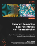
The vector, as represented on the Bloch sphere, is at the equator of the X-axis. This location is called the |+⟩ state:
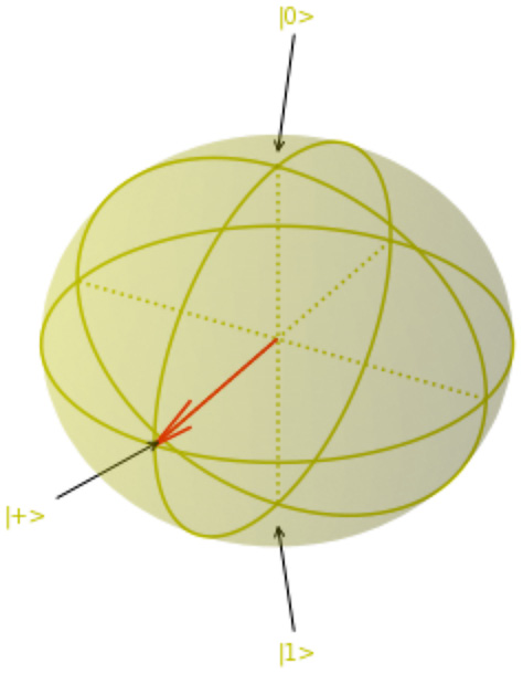
Figure 6.5 – Bloch sphere representing the qubit at the |+⟩ state
- For clarity, let’s visualize the h operator’s effect on the quantum state of the qubit. This operator, as mentioned earlier, is also called the Hadamard gate and provides a rotation around the X, Y, and Z-axes simultaneously. It is hard to visualize this, but the following diagram may help. We discussed the z operator and the x (or NOT) operator. The Hadamard gate is equivalent to a rotation with the axis halfway between the Z and X-axes:

Figure 6.6 – Effect of using the Hadamard gate
In the preceding diagram, we applied the Hadamard gate twice:
- (1.) Starting at the |0⟩ state, the Hadamard moves the qubit to the |+⟩ state.
- (2.) Starting at the |+⟩ state, the Hadamard moves the qubit back to the |0⟩ state.
- Now, let’s re-prepare the plus state and store it in the arr_plus variable:
arr_plus=arr_h @ arr_0
print(arr_plus)
Output:
[[0.70710678+0.j]
 [0.70710678+0.j]]
- Now, let’s use the arr_z matrix, which represents the Pauli-Z matrix. This is also represented by the z gate and is a π rotation around the Z-axis. We can use this to rotate the qubit from the |+⟩ state to the |-⟩ state. This is equivalent to matrix multiplication:

The same process can be represented with the following code:
arr_minus=draw_bloch(arr_z @ arr_plus)
Output:
Matrix:
[[ 0.70710678+0.j]
 [-0.70710678+0.j]]
The Bloch sphere showing the qubit in the |-⟩ state is as follows:

Figure 6.7 – Bloch sphere showing the qubit state of |-⟩
- Our final example will be to rotate the qubit vector π/4 degrees using the t gate or the arr_t matrix. This is equivalent to the following matrix multiplication:

Note the following:

The same process can be done with the following code:
arr_r=draw_bloch(arr_t @ arr_minus)
Output:
Matrix:
[[ 0.70710678+0.j ]
 [-0.5       -0.5j]]
The final position on the qubit vector is on the equator of the Bloch sphere rotated π/4 from the |-⟩ state or rotated at an angle of 5/8 π from the |+⟩ state, as shown here:

Figure 6.8 – Bloch sphere showing the final state with a z-rotation angle of φ = (5/8) π
At this point, we have studied the behavior of one qubit with some simple rotations of the vector representing the qubit. We used the Bloch sphere to visualize the state vector of the qubit and also looked at the equivalent mathematical representation of the rotations using their equivalent unitary matrices.
Now, let’s build the same single-qubit rotations using the Amazon Braket Circuit() function and their equivalent quantum gates.
Using quantum gates in a quantum circuit
In the previous section, we worked with a single qubit, performed various operations on that single-qubit using matrix multiplication, and showed the results on a Bloch sphere. Now, let’s look at the same process using quantum gates using the Amazon Braket Circuit() function. We will use the custom draw_circuit() function, which will allow you to submit a single-qubit quantum circuit that will display the quantum circuit diagram, show the results after executing it using the LocalSimulator(), and display a Bloch sphere.
Let’s get started:
- The draw_circuit() function is provided in this chapter’s code. We will use this here to make drawing and executing the single gate circuits easier. The following is the relevant code:
def draw_circuit(circ):
    circ=circ.state_vector()
    print(circ)
    device = LocalSimulator()
    result = device.run(circ).result()
    arr_r=np.array(
      [[result.values[0][0]],[result.values[0][1]]])
    draw_bloch(arr_r)
- We can run the identity gate on the 0th qubit by using i(0). This will leave the original qubit state of |0⟩ unchanged:
circ=Circuit().i(0)
draw_circuit(circ)
Output:
T  : |0|
q0 : -I-
T  : |0|
Matrix:
[[1.+0.j]
 [0.+0.j]]
As you can see, the circuit is represented in the first three lines and that after q0, we have only one gate, I. T represents the depth of the circuit. The resulting matrix shows that the state is still |0⟩. The following diagram shows the resulting Bloch sphere showing the same:

Figure 6.9 – Bloch sphere showing the |0⟩ state
- Now that we know how some of the other unitary single-qubit gates work, let’s try to bring the qubit to the |-⟩ state. We have several options, but here, we will start with a Hadamard gate, then a Z gate. Both gates will be applied to qubit 0. This provides the appropriate rotations to bring the qubit state to the |+⟩ state and then provides a π rotation around the Z-axis to bring the qubit to the |-⟩ state:
circ=Circuit().h(0).z(0)
draw_circuit(circ)
Output:
T  : |0|1|
q0 : -H-Z-
T  : |0|1|
Matrix:
[[ 0.70710678+0.j]
 [-0.70710678+0.j]]
The qubit is now at the |-⟩ state. The Bloch sphere should also confirm this:
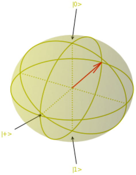
Figure 6.10 – Bloch sphere showing the |-⟩ state
- Starting at the |0⟩ state, we can also try applying a Hadamard with a T gate, which is a π/4 rotation around the Z-axis:
circ=Circuit().h(0).t(0)
draw_circuit(circ)
Output:
T  : |0|1|
q0 : -H-T-
T  : |0|1|
Matrix:
[[0.70710678+0.j ]
 [0.5       +0.5j]]
The Bloch sphere shows the qubit state as follows:
Figure 6.11 – Bloch sphere after starting at |0⟩ and applying an H and a T gate
- Now, let’s look at the effect of the circuit by starting at the |0⟩ state and then applying the X, H, and S gates. The S gate is a π/2 rotation around the Z-axis. So, in this case, we move to the |1⟩ state due to the X gate, then the |-⟩ state because of the Hadamard, and then a π/2 degree rotation around the Z-axis (around the equator) to the |-i⟩ state. This is equivalent to the following matrix multiplication:

The equivalent circuit can be set up with the following code:
circ=Circuit().x(0).h(0).s(0)
draw_circuit(circ)
Output:
T  : |0|1|2|
q0 : -X-H-S-
T  : |0|1|2|
Matrix:
[[0.70710678+0.j        0.]
 [0.        -0.70710678j]]
The Bloch sphere representation is as follows:
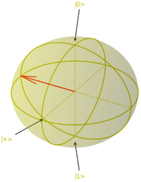
Figure 6.12 – Bloch sphere in the |-i⟩ state
Most of the gates we have used so far had predefined rotations around the X or Z-axis. We can also apply specific angle rotations to the qubit around any of the three axes. We will look at the rotation functions using an example in the next section.
Single-qubit gate rotation example – the Bloch Clock
We can apply specific rotations around each axis using the rx(q,θ), ry(q,θ), or rz(q,φ) gates. Here, q is the qubit number, and θ and φ are the rotation angles in radians. Thus, any value from 0 to 2π or 0 to -2π will fully rotate the vector around that axis back to the starting point. Any multiples will cause multiple rotations.
To try out two new gates RY and RZ, represented by the following functions, ry() and rz(), we will encode the time of the day in the Bloch sphere. Looking back at Figure 6.1, we will use the rotation around the Y-axis or the θ angle to represent the hour of the day and the φ angle to represent the minutes.
Representing the hour of the day using θ
Thus, through the day, the qubit vector will spiral down from the |0⟩ state, representing midnight, to the equator, which will be at noon, and then continue to spiral down to the |1⟩ state toward midnight again. The top of the hour (:00) will be represented with a phase of π degrees. Thus, we will use the ry(θ) gate to rotate the qubit vector in the -y direction to represent the top of the hour. Thus, θ represents a fraction of the 24 hours through the day.
Representing the minutes and seconds using φ
To represent the clockwise rotation of the minutes and seconds around the Z-axis, we will rotate the φ angle in the reverse direction using the rz() gate, starting at π degrees. The bloch_clock() code is as follows:
def bloch_clock():
    from time import gmtime
    import datetime
    import numpy as np
    time=gmtime()
    #set to EDT
    HR=time.tm_hour-4
    if HR<0:
        HR=HR+24
    MIN=time.tm_min
    SEC=time.tm_sec
    print''HR'',HR,''MIN'',MIN,''SEC'', SEC,''ED'')
    circ=Circuit().ry(0,-(HR+MIN/60
      +SEC/3600)*np.pi/24).rz(0,-(MIN+SEC/60)*2*np.pi/60)
    draw_circuit(circ)
Output:
HR: 11 MIN: 35 SEC: 30 EDT
T  : |    0    |    1    |
q0 : -Ry(-1.52)-Rz(-3.72)-
T  : |    0    |    1    |
Additional result types: StateVector
Matrix:
[[-0.20612405+0.69586314j]
 [ 0.19539087+0.65962852j]]
For 11:35:30, the Bloch Clock shows the following output:
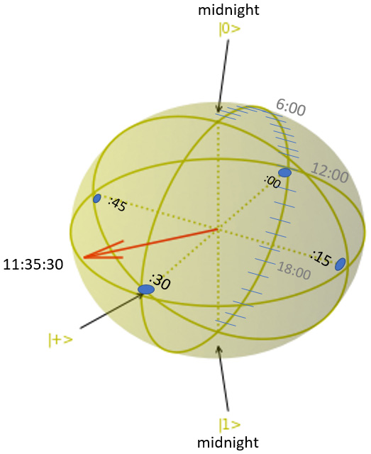
Figure 6.13–- Bloch Clock showing 11:35:30
You can get your own time on the Bloch sphere by running bloch_clock(). Please adjust the hour to your time zone by adjusting the constant in the HR=time.tm_hour-4 line.
We are now going to start dealing with multiple qubits. It is not practical to show a multiple qubit state space using a Bloch sphere, even though there are different ways to split the information into phase diagrams or show partial information on a single sphere. In any case, next, we will focus on using larger matrices that represent more qubits and also show how matrix multiplication can easily be represented by using gates on a quantum circuit.
Building multiple qubit quantum circuits
In this section, we will build the matrix math for a full circuit that contains multiple qubits and then show how the results match the output from a quantum gate circuit. So far, we have used matrix multiplication and the @ symbol to multiply the original state with a series of matrices that represent unitary operators or quantum gates on one qubit. When we are dealing with multiple qubits, the vector space of each will have to be multiplied together using the tensor product, which is typically represented by the ⊗ symbol. We will use the NumPy kron() function to calculate this:
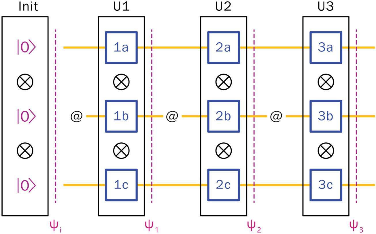
Figure 6.14 – Matrix multiplication of a quantum gate circuit
The preceding diagram shows a sample quantum circuit with various gates (squares) each representing a 2x2 matrix. The initial state on each qubit is going to be the |0⟩ state. To represent this quantum circuit using matrix multiplication, we can use the tensor product between each of the gates to create a unitary matrix that represents a column of gates. Thus, to create U1, we need the tensor product between 1a, 1b, and 1c. To get the ![]() state, we need to apply the unitary matrix, U1, to the prior state,
state, we need to apply the unitary matrix, U1, to the prior state, ![]() , using matrix multiplication. Each subsequent column of gates is applied the same way to the previous state, or they can be multiplied together as a single unitary and then applied once to the initial state to get the final state of the circuit. Let’s build the matrix math of this circuit step by step:
, using matrix multiplication. Each subsequent column of gates is applied the same way to the previous state, or they can be multiplied together as a single unitary and then applied once to the initial state to get the final state of the circuit. Let’s build the matrix math of this circuit step by step:
- Let’s start with the tensor product of the initial state, (
 ), of the qubits. Since we have three qubits, this will be as follows:
For n qubits, we could write the following general expression:

- The next unitary will be given by the following equation:

- The next state,
 , is given by multiplying the matrix of the initial state,
  , with U1. Thus, we get the following:
- The next state,
 , is given by multiplying the matrix of the state
  with U2. Thus, we get the following:

We also get the following:

- Finally, the
 state is given by multiplying the matrix of the state,
  , with U3. Thus, we get the following equation:

We also get the following equation:
- As mentioned earlier, we can also combine all the gate operations into a single unitary matrix and then apply that to the initial state. Thus, another way to represent
 would be as follows:
This can also be expanded for clarity:

Having looked at the general process of matrix multiplication to represent a quantum circuit, in the next section, we will use this process to get the final state of a specific circuit with single-qubit and two-qubit gates. You should keep in mind that to ensure each unitary has the correct size, any missing gates can be filled with the I identity matrix. Technically, in an actual quantum circuit, gates will be stacked to the left to eliminate any gaps, unless this is prevented due to a multiple qubit gate.
Three-qubit circuit example
We will now use what we have learned to create a slightly more complicated quantum circuit on three qubits. The diagram below shows this sample circuit with four unitary gate operations on the three qubits. The first and last operation has all Hadamard gates, while U2 has single qubit gates, and U3 has a CNOT gate with an Identity gate. We have looked at all these steps already, but now we will put it together to get the final state of this quantum circuit through both matrix multiplication and then finally using quantum gates.

Figure 6.15 – Sample circuit to create
Now, let’s use this information to learn how to calculate the end state matrix for a set of gates in a three-qubit quantum circuit, as shown in the preceding diagram:
- Starting with the bottom two qubit states of|0⟩ and then adding the third top qubit state of |0⟩, we must use the NumPy kron() function twice:
arr_psi_i=np.kron(arr_0,np.kron(arr_0, arr_0))
print(arr_psi_i)
Output:
[[1.+0.j]
 [0.+0.j]
 [0.+0.j]
 [0.+0.j]
 [0.+0.j]
 [0.+0.j]
 [0.+0.j]
 [0.+0.j]]
The equivalent matrix representation involves the tensor product of the three matrices:

- Now, let’s add Hadamards or H-gate, which is represented by the
 matrix, to all the qubits. This will bring them to an equal superposition state.
Thus, the first unitary matrix will be the tensor product of three Hadamard gates:
arr_U1=np.kron(arr_h,np.kron(arr_h, arr_h))
print(arr_U1)
Output:
[[ 0.35355339  0.35355339  0.35355339  0.35355339  0.35355339  0.35355339   0.35355339  0.35355339]
 [ 0.35355339 -0.35355339  0.35355339 -0.35355339  0.35355339 -0.35355339   0.35355339 -0.35355339]
 [ 0.35355339  0.35355339 -0.35355339 -0.35355339  0.35355339  0.35355339  -0.35355339 -0.35355339]
 [ 0.35355339 -0.35355339 -0.35355339  0.35355339  0.35355339 -0.35355339  -0.35355339  0.35355339]
 [ 0.35355339  0.35355339  0.35355339  0.35355339 -0.35355339 -0.35355339  -0.35355339 -0.35355339]
 [ 0.35355339 -0.35355339  0.35355339 -0.35355339 -0.35355339  0.35355339  -0.35355339  0.35355339]
 [ 0.35355339  0.35355339 -0.35355339 -0.35355339 -0.35355339 -0.35355339   0.35355339  0.35355339]
 [ 0.35355339 -0.35355339 -0.35355339  0.35355339 -0.35355339  0.35355339   0.35355339 -0.35355339]]
- To get the state, we need to look at the effect the arr_U1 unitary matrix has on the initial state, arr_psi_i. This is given by the following matrix multiplication:

- To run the circuit, let’s use the LocalSimulator() and run_circuit_local() functions, which can be found in the code for this chapter, to produce the results:
def run_circuit_local(circ):
    # This function prints the quantum circuit and
    # calculates the final state vector
    # This can be used for multiple qubits and only
    # uses the local simulator
    # The Bloch sphere is not printed
    circ=circ.state_vector()
    print(circ)
    device = LocalSimulator()
    result = device.run(circ).result()
    arr_r=np.array(result.values).T
    print(arr_r)
    return(arr_r)
- Now, we can create the circuit equivalent, as shown here:
circ_psi_1=Circuit().h([0,1,2])
result=run_circuit_local(circ_psi_1)
Output:
T  : |0|
q0 : -H-
q1 : -H-
q2 : -H-
T  : |0|
Additional result types: StateVector
[[0.35355339+0.j]
 [0.35355339+0.j]
 [0.35355339+0.j]
 [0.35355339+0.j]
 [0.35355339+0.j]
 [0.35355339+0.j]
 [0.35355339+0.j]
 [0.35355339+0.j]]
- Now, let’s apply three different single-qubit gates to create a unitary, U2. Let’s use gates x()
 , y()
, y()  , and z()
  from the top down. The following matrix multiplication is involved:
The matrix code to build U2 is as follows:
arr_U2=np.kron(arr_x,np.kron(arr_y, arr_z))
print(arr_U2)
Output:
[[ 0.+0.j  0.+0.j  0.+0.j  0.+0.j  0.+0.j  0.+0.j  0.-1.j  0.+0.j]
 [ 0.+0.j -0.+0.j  0.+0.j  0.+0.j  0.+0.j -0.+0.j  0.+0.j  0.+1.j]
 [ 0.+0.j  0.+0.j  0.+0.j  0.+0.j  0.+1.j  0.+0.j  0.+0.j  0.+0.j]
 [ 0.+0.j  0.-0.j  0.+0.j -0.+0.j  0.+0.j  0.-1.j  0.+0.j -0.+0.j]
 [ 0.+0.j  0.+0.j  0.-1.j  0.+0.j  0.+0.j  0.+0.j  0.+0.j  0.+0.j]
 [ 0.+0.j -0.+0.j  0.+0.j  0.+1.j  0.+0.j -0.+0.j  0.+0.j  0.+0.j]
 [ 0.+1.j  0.+0.j  0.+0.j  0.+0.j  0.+0.j  0.+0.j  0.+0.j  0.+0.j]
 [ 0.+0.j  0.-1.j  0.+0.j -0.+0.j  0.+0.j  0.-0.j  0.+0.j -0.+0.j]]
- The following code develops arr_psi_2, which will apply the U2 operator to the last state, arr_psi_1:
arr_psi_2=arr_U2 @ arr_psi_1
print(arr_psi_2)
Output:
[[0.-0.35355339j]
 [0.+0.35355339j]
 [0.+0.35355339j]
 [0.-0.35355339j]
 [0.-0.35355339j]
 [0.+0.35355339j]
 [0.+0.35355339j]
 [0.-0.35355339j]]
- The following is the same process using quantum gates:
circ_psi_2=circ_psi_1.x(0).y(1).z(2)
result=run_circuit_local(circ_psi_2)
Output:
T  : |0|1|
q0 : -H-X-
q1 : -H-Y-
q2 : -H-Z-
T  : |0|1|
Additional result types: StateVector
[[0.-0.35355339j]
 [0.+0.35355339j]
 [0.+0.35355339j]
 [0.-0.35355339j]
 [0.-0.35355339j]
 [0.+0.35355339j]
 [0.+0.35355339j]
 [0.-0.35355339j]]
As you can see, the resulting state vector from the circuit is the same as that when using matrix multiplication.
- So far, we have only applied the Hadamard gates and single-qubit gates. As you can see, we have eight amplitudes from the three qubits. As you may recall, the number of amplitudes is 2n where n is the number of qubits, and is one feature that gives quantum computers their advantage. We can now apply a CX or CNOT gate on two qubits with the cnot() function. This is a two-qubit gate. The following is its matrix representation. In this case, the first qubit is the control and the second qubit is the target. If the control qubit has a state of |1⟩, then the second qubit will perform an X operation and flip the qubit:

We will simply show how a CNOT gate works in the following steps before using this gate in the circuit:
- First, we must create the arr_cx array as the CNOT matrix:
arr_cx=np.array([[1, 0, 0, 0], [0, 1, 0, 0], [0, 0, 0, 1], [0, 0, 1, 0]])
- To prove this point, let’s create a state of |10⟩:
arr_10= np.kron(arr_1, arr_0)
print(arr_10)
Output:
[[0.+0.j]
 [0.+0.j]
 [1.+0.j]
 [0.+0.j]]
- Now, we can perform the cnot() operation on arr_10 or |10⟩:
arr_11= arr_cx @ arr_10
print(arr_11)
Output:
[[0.+0.j]
 [0.+0.j]
 [0.+0.j]
 [1.+0.j]]
Since the first qubit is in a state of |1⟩, the second qubit will change states from |0⟩ to |1⟩. Thus, we will see a |11⟩ resulting state.
- Back to our three-qubit circuit, since we want to apply the cnot() gate on qubit 1 and 2 with the and use the identity i() gate
 on qubit 0 so that we can create the third unitary, U3:

The code is as follows:
arr_U3=np.kron(arr_i,arr_cx)
print(arr_U3)
Output:
[[1 0 0 0 0 0 0 0]
 [0 1 0 0 0 0 0 0]
 [0 0 0 1 0 0 0 0]
 [0 0 1 0 0 0 0 0]
 [0 0 0 0 1 0 0 0]
 [0 0 0 0 0 1 0 0]
 [0 0 0 0 0 0 0 1]
 [0 0 0 0 0 0 1 0]]
- The final state, , is then stored in arr_psi_3 using the following code:
arr_psi_3=arr_U3 @ arr_psi_2
print(arr_psi_3)
Output:
[[0.-0.35355339j]
 [0.+0.35355339j]
 [0.-0.35355339j]
 [0.+0.35355339j]
 [0.-0.35355339j]
 [0.+0.35355339j]
 [0.-0.35355339j]
 [0.+0.35355339j]]
- The same can be done using the quantum gates:
circ_psi_3=circ_psi_2.i(0).cnot(1,2)
result=run_circuit_local(circ_psi_3)
Output:
T  : |0|1|2|
q0 : -H-X-I-
q1 : -H-Y-C-
          |
q2 : -H-Z-X-
T  : |0|1|2|
Additional result types: StateVector
[[0.-0.35355339j]
 [0.+0.35355339j]
 [0.-0.35355339j]
 [0.+0.35355339j]
 [0.-0.35355339j]
 [0.+0.35355339j]
 [0.-0.35355339j]
[0.+0.35355339j]]- The final step is to add Hadamard gates to each qubit again and measure the final circuit. In this case, we will just create the circuit from scratch to show how convenient it is to use gate circuits to represent all the matrix math that is happening in the background:
circ_psi_3=Circuit().h([0,1,2]).x(0).y(1).z(2).i(0).cnot(1,2).h([0,1,2])
arr_psi_3=run_circuit_local(circ_psi_3)
Output:
T  : |0|1|2|3|
q0 : -H-X-I-H-
q1 : -H-Y-C-H-
          |
q2 : -H-Z-X-H-
T  : |0|1|2|3|
Additional result types: StateVector
[[0.-2.36158002e-17j]
 [0.-1.00000000e+00j]
 [0.-1.26316153e-34j]
 [0.-9.52420783e-18j]
 [0.+0.00000000e+00j]
 [0.+0.00000000e+00j]
 [0.+0.00000000e+00j]
[0.+0.00000000e+00j]]- We can determine the probabilities of each state by squaring each of the amplitudes. Here, the resulting state is given by the following equation:

- Below we will now repeat the process using a quantum circuit and adding the gates. This will help us avoid all the matrix multiplication we did in the previous steps. On a simulator or an error-free quantum computer, we should get 001 100% of the time:
circ_psi_3=Circuit().h([0,1,2]).x(0).y(1).z(2).i(0).cnot(1,2).h([0,1,2])
device = LocalSimulator()
result = device.run(circ_psi_3, shots=1000).result()
counts = result.measurement_counts
print(counts)
# plot using Counter
plt.bar(counts.keys(), counts.values());
plt.xlabel('v'lue')'
plt.ylabel('c'unts')'
Output:
Counter({'0'1':'1000})The resulting bar chart also shows the same result of getting 001 only:

Figure 6.16 – Resulting probabilities after measuring the circuit using LocalSimulator()
With that, we have completed several steps showing how quantum gates are equivalent to specific matrices and that the structure of a quantum circuit can be simulated using a step-by-step process, which involves creating unitary matrix operators that act on the previous state vector. Initially, we looked at the process of matrix multiplication for a single-qubit example. We also saw that we can extend this process to multiple qubits, so long as we take the tensor product of each column of gates to ensure they are converted into a unitary matrix. Then, we multiplied the matrix of the initial state with the first unitary, which applies Hadamards to the three qubits to bring them into superposition. We did the same to the second state, which applies the single-qubit x, y, and z gates, and then the third, which applies an identity gate to the first qubit, followed by a two-qubit control gate or the CNOT gate on the next two qubits, which entangle the two qubits together. The final step involved adding Hadamards to all the qubits to remove the superposition, just before the circuit is measured. We started with a state of all zeros and returned with 001, which is measured 100% of the time through this circuit.
This simple circuit lays the foundation for the next section, where we will look at a modified example inspired by the Google Supremacy experiment.
Example inspired by the Google Supremacy experiment
We will apply what we have learned about gate operations to an experiment inspired by the Google Supremacy experiment. The paper titled Quantum supremacy using a programmable superconducting processor was published in Nature in October 2019. The links to this paper and the counter-claim by IBM can be found in the Further reading section. This is a good example to start with, as it does not require a specific quantum circuit, and can also explain, to some extent, the process used in the widely talked about experiment.
The actual Google experiment
The Google experiment used an alternating set of randomly selected single-qubit gates (![]() ). It entangled one of a different set of interconnected qubits using a combination of iSWAP and a CrZ (π /6) gate that had been calibrated for minimum error between that specific pair of qubits. This includes five other rotation angles that I have not shown.
). It entangled one of a different set of interconnected qubits using a combination of iSWAP and a CrZ (π /6) gate that had been calibrated for minimum error between that specific pair of qubits. This includes five other rotation angles that I have not shown.
The following equation shows the matrices for the aforementioned ![]() and
and ![]() gates:
gates:

The ![]() gate is defined as
gate is defined as 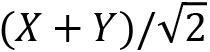 .
.
The two-qubit gate uses a combination of an iSWAP and CrZ(![]() ), where y = π /6. Other rotations for optimizing the two-qubit gate for the highest fidelity of the qubit pair interaction have not been shown here:
), where y = π /6. Other rotations for optimizing the two-qubit gate for the highest fidelity of the qubit pair interaction have not been shown here:

The single and multiple qubit gates were repeated r times, where r=20. Since this experiment was done on their 54-qubit Sycamore quantum processor with one qubit not functioning properly, this led to a 53-qubit system and thus 253 different possible states. As we have seen, based on the matrix calculations, to simulate one step of 53 gates on 53 qubits, we must find the tensor products of 53 gates, which creates a matrix of size 253x253. The team stated that the RAM availability in the Jülich supercomputer (with 100,000 cores and 250 terabytes) limited calculations to up to 48 qubits. Beyond that, other hybrid methods were used. The claim that was made was that with the quantum processor, these calculations, with r=20 and 1 million measurement samples, were performed in 200 seconds, while classical processors would require 50 trillion core hours and consume 1 petawatt hour of energy (estimated to take 10,000 years with a million-core supercomputer). Counterclaims were made by IBM and other teams.
Circuit implementation on Amazon Braket
For our purposes, we will create a circuit where we can randomly select single-qubit gates for each qubit, and then use the two-qubit CNOT gate to entangle qubits. We will use identity gates so that we can move the CNOT gates up and down, thus randomly entangling different sets of qubits. The following diagram shows two sample repetitions of this circuit. We will calculate the full circuit’s unitary using tensor products and matrix multiplication, along with its equivalent gate circuit, and run it on the local simulator and the Amazon Braket SV1 and TN1 simulators. Finally, we will look at the performance of both the Rigetti and IonQ quantum devices:
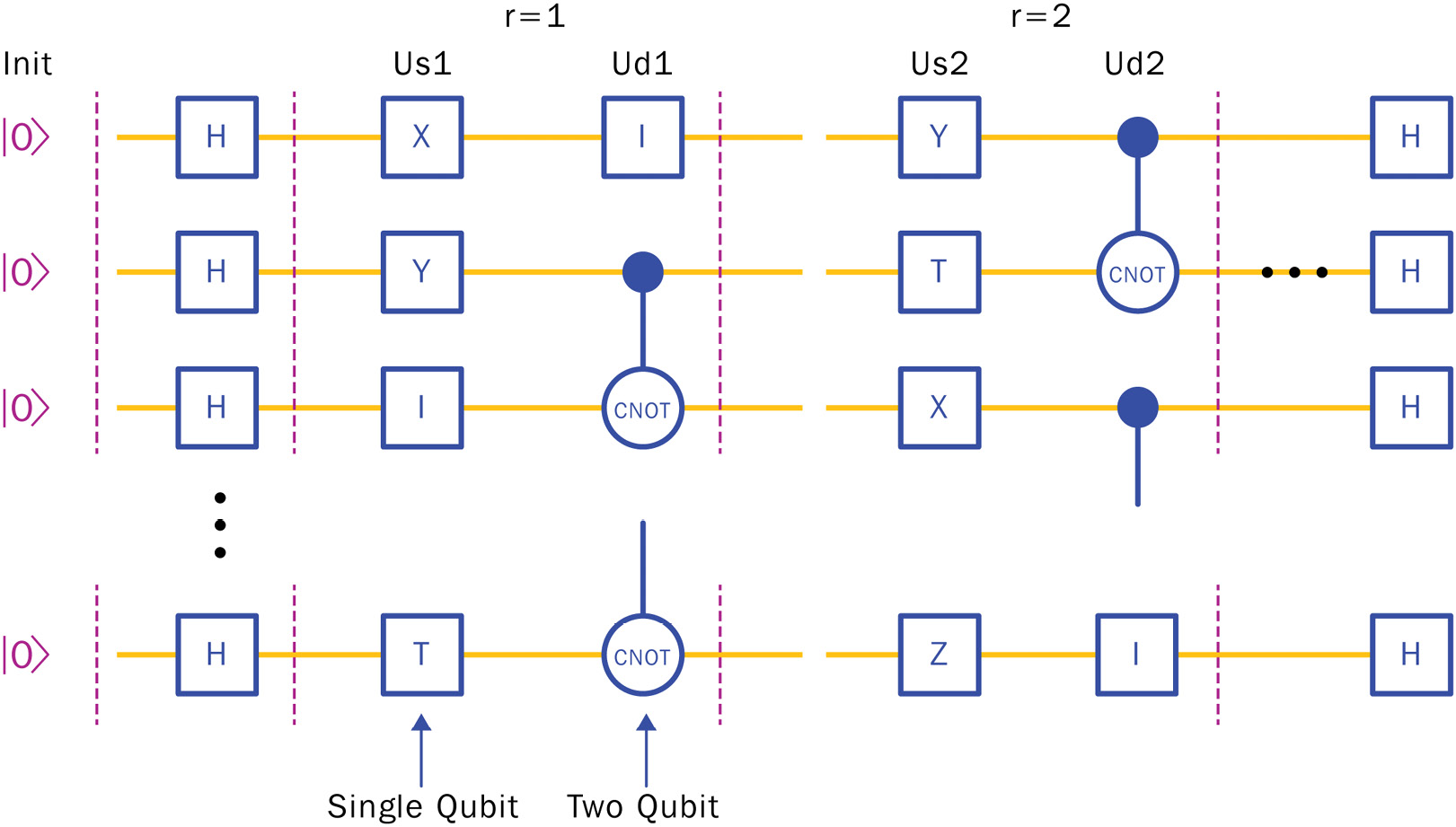
Figure 6.17 – Google Quantum supremacy-inspired circuit with alternating random single-qubit gates (X, Y, Z, I, T) and randomly placed CNOT gates repeated r times
The function that creates the circuit and equivalent unitary for the full circuit is qc_rand() and is provided in the code for this chapter. All you need to do is provide the number of qubits and the number of repeats, r, in the circuit. The last parameter is a Boolean to create the unitary. This is True by default, but if your classical processor cannot generate the unitary (around 11 or 12 qubits), set Matrix=False.
We will start with seven qubits, q=7, and set the repeats to two, r=2. This allows us to see all the different options with good results.
Note – Code Preparation
As you follow along, do not accidentally execute a run on the quantum devices (the IonQ Device and Aspen) unless you are willing to budget $32 and $1.42 for this configuration.
Execute the available_devices() function to ensure you have the latest device names, adjust the code accordingly, and run experiments on the devices available at the time you execute the code.
Please execute the estimate_cost() or estimate_cost_measured_qubits() function before running these devices with the appropriate number of qubits and desired number of shots. In the following code, I have executed these functions to give you price estimates.
At the end of this section, I will go over some insights as to which configurations do not work or give poor results. Then, you can try out different configurations at the end of this section, though note that the IonQ execution can get very expensive. It can cost up to $100 if you’re executing the circuit on 11 qubits with the maximum number of suggested shots at 10,000. Executing a 32-qubit circuit on Rigetti with 100,000 shots can cost $35.00.
Execution results for a single 7x2 circuit
We will start with a small circuit with 7 qubits and repeat the alternating single and two-qubit gates twice. Since we will also apply Hadamard gates, this is a gate depth of 6. Due to the number of qubits, the circuit should work on all local devices, simulators, and quantum devices and provide good results.
Note – Each Run Will Generate a Different Circuit
Since the circuit is randomly generated, when you run the code, you will end up generating a different circuit with different results. Have fun!
Later, we will compare the results when using larger circuits.
Execution on a local device
In this section, we will review the code as we implement the circuit using matrix math and use simulators on local devices. Let’s get started:
- To create a circuit for 7 qubits and repeat the circuit twice, we must enter the following code:
q=7
r=2
Ufinal, g_circ=qc_rand(q,r)
The equation returns both the randomly generated unitary, Ufinal, and its equivalent quantum circuit, g_circ.
- We can view this circuit by printing it:
print(g_circ)
Output:
T  : |0|1|2|3|4|5|
q0 : -H-X-I-X-C-H-
              |
q1 : -H-I-C-X-X-H-
          |
q2 : -H-I-X-X-C-H-
              |
q3 : -H-T-C-T-X-H-
          |
q4 : -H-X-X-X-C-H-
              |
q5 : -H-X-C-X-X-H-
          |
q6 : -H-Z-X-Z-I-H-
T  : |0|1|2|3|4|5|
Notice that the gate position, T:0, has the Hadamard gates, the T:1 position has the random single-qubit gates (X,I,T, and Z), and the T:2 position has the two-qubit CNOT gates. Positions T:3 and T:4 repeat with a new set of single-qubit gates and a different positioning of the CNOT gates to entangle a different set of qubits. Finally, T:5 has Hadamard gates on all its qubits. We can use the values of T to determine the gate depth of the circuit or use the g_circ.depth function.
- We can also view a portion of the 27 x 27 unitary matrix, as follows:
print(Ufinal)
Output:
[[-7.13653841e-20+2.87907611e-19j  7.13653841e-20+5.79454127e-19j
  -5.00000000e-01-5.00000000e-01j ...  7.13653841e-20-5.79454127e-19j
   1.42730768e-19-2.89363173e-18j  0.00000000e+00+0.00000000e+00j]
 [ 7.13653841e-20-2.87907611e-19j  5.00000000e-01+5.00000000e-01j
  -7.13653841e-20-5.79454127e-19j ... -1.80608886e-18+1.44681586e-18j
   0.00000000e+00+0.00000000e+00j  1.42730768e-19+5.75815222e-19j]
 [ 1.66335809e-18-2.02263109e-18j  7.13653841e-20-5.79454127e-19j
   7.13653841e-20-1.44681586e-18j ...  7.13653841e-20+5.79454127e-19j
   1.42730768e-19+1.15890825e-18j  0.00000000e+00+0.00000000e+00j]
 ...
 [-7.13653841e-20+2.87907611e-19j  1.80608886e-18+1.44681586e-18j
   7.13653841e-20+5.79454127e-19j ...  5.27553581e-18-1.44681586e-18j
   0.00000000e+00+0.00000000e+00j -1.42730768e-19-5.75815222e-19j]
 [-8.60225200e-18+5.49207804e-18j -7.13653841e-20+5.79454127e-19j
  -7.13653841e-20+1.44681586e-18j ... -7.13653841e-20-5.79454127e-19j
  -1.42730768e-19-1.15890825e-18j  0.00000000e+00+0.00000000e+00j]
 [-7.13653841e-20-2.87907611e-19j  7.13653841e-20-1.44681586e-18j
   7.13653841e-20-5.79454127e-19j ...  7.13653841e-20+1.44681586e-18j
   0.00000000e+00+0.00000000e+00j -1.42730768e-19+5.75815222e-19j]]
Keep in mind that this is a 27 x 27 (128x128) matrix.
- Now, we can apply the unitary to an array that represents the initial state of
 . The following code is mostly printing the results by squaring each amplitude in the results to convert them from amplitudes into probability of measurements, then turning the results into a percentage for plotting:
n=q
x_val=[]
y_val=[]
init_arr=np.zeros((2**n,1))
init_arr[0]=1
shots=1000
result=shots*np.square(np.abs(Ufinal @ init_arr))
y_val_t=(result.T.ravel())
for i in range (len(y_val_t)):
    y_val.append(int(100*y_val_t[i]/shots))
x_val=range(2**n)
x_index=np.argsort(x_val)
for i in (x_index):
    if y_val[i]>=1:
        print(x_val[i],':', y_val[i])
plt.bar(x_val, y_val)
plt.xlabel('states');
plt.ylabel('percent');
plt.title('q='+str(n)+', r='+str(r)+
          ' Unitary Matrix Multiplication')
plt.rcParams["figure.figsize"] = (30,30)
plt.rcParams['figure.dpi'] = 150
plt.show()
Output:
6 : 49
30 : 49
There are a total of 128 possible states or values based on the seven qubits that are used. This circuit produces two results: one is 6 with a probability of 49% and the other is 30 with a probability of 49%. These values have been rounded, and there might be other probabilities smaller than 1% that have been ignored for our purposes:

Figure 6.18 – Resulting state probabilities from matrix multiplication
- Now, let’s convert the unitary matrix into a circuit. This can be done using a function provided in Amazon Braket called .unitary(matrix=Unitary, targets=targets), where Unitary is the matrix being added to the circuit and targets is a list of all the qubits that the unitary will span. In our case, targets=[0,1,2,3,4,5,6]:
targets=[]
circ_Ufinal=Circuit()
for I in range (n):
    targets.append(i)
circ_Ufinal=circ_Ufinal.unitary(matrix=Ufinal,
                                targets=targets)
print(circ_Ufinal)
Output:
T  : |0|
q0 : -U-
      |
q1 : -U-
      |
q2 : -U-
      |
q3 : -U-
      |
q4 : -U-
      |
q5 : -U-
      |
q6 : -U-
T  : |0|
The preceding output shows a quantum circuit built out of only one unitary matrix.
- Now, we will see that executing this unitary circuit is equivalent to the matrix multiplication we did in Step 4. We will set the device as a LocalSimulator and then run the circ_Ufinal circuit using device.run(). Please note that in the code, we are converting the resulting counts into percentages using y_val.append(int(100*i/shots)) and only showing values equal to or greater than 1% to keep the output constrained using if y_val[i]>=1:
device = LocalSimulator()
shots=1000
result = device.run(circ_Ufinal, shots=shots).result()
counts = result.measurement_counts
#print(counts)
x_val=[]
y_val=[]
for i in (counts.keys()):
    x_val.append(int(i,2))
for i in (counts.values()):
    y_val.append(int(100*i/shots))
x_index=np.argsort(x_val)
for i in (x_index):
    if y_val[i]>=1:
        print(x_val[i],':', y_val[i])
plt.bar(x_val, y_val, color='b')
plt.title('q='+str(n)+', r='+str(r)+
          ' Unitary on LocalSimulator')
plt.xlabel('states');
plt.ylabel('percent');
plt.rcParams["figure.figsize"] = (20,10)
plt.rcParams['figure.dpi'] = 300
plt.show()
Output:
6 : 52
30 : 47
Notice that the results in the output are the same two values as in Step 4; that is, 6 and 30. However, the percentages are a bit different due to all the other smaller probabilities being rounded:
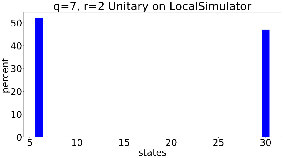
Figure 6.19 – Resulting state probabilities after using a gate circuit based on the single unitary
- Now, we will run the gate circuit, g_circ, that was generated in Step 1. Here, we only show the relevant part of the circuit that gets the results. The rest of the code is similar to that in Step 6. The full code is available in this chapter’s code repository:
result = device.run(g_circ, shots=shots).result()
Output:
6 : 48
30 : 52
Again, the two values that are in the output have approximately the same percentages they had previously:

Figure 6.20 – The resulting state probabilities after using the gate quantum circuit on LocalSimulator
With that, we have evaluated the quantum circuit using matrix math and done the same on local simulators. In the next subsection, we will use the Amazon Braket simulators.
Execution on Amazon Braket simulators
In this section, we will continue running the 7 x 2 circuit on both the SV1 and TN1 Amazon Braket simulators:
- First, we will run the same unitary circuit on the SV1 simulator. The necessary code required is shown here:
- The following code will assign the device to SV1 using the set_device() function that is provided in the code for this chapter. The cost for the device can be found using the estimate_cost() function provided in the code:
device_name='SV1'
device=set_device(device_name)
estimate_cost(device)
Output:
Device('name': SV1, 'arn': arn:aws:braket:::device/quantum-simulator/amazon/sv1)
simulator cost per  minute : $ 0.075
total cost cannot be estimated- Now, we can calculate the estimated number of shots using the estimate_cost_measured_qubits() function, which is provided in the code for this chapter:
shots=estimate_cost_measured_qubits(device, n)
Output:
max shots: 100000
for 7 measured qubits the number of shots recommended: 3,200
simulator cost per  minute : $ 0.075
total cost cannot be estimated
- Now, let’s run the unitary circuit, circ_Ufinal, on SV1. Note that before executing an Amazon Braket device, ensure that you have assigned the values of s3_folder:
title='q='+str(n)+', r='+str(r)+' Unitary on '+device_name
result=run_circuit(device, circ_Ufinal, shots, s3_folder, title, False)
Output:
6 : 50
30 : 49
This results in the following chart:

Figure 6.21 – Resulting state probabilities after using the unitary circuit on SV1
- We will repeat the same process using g_circ on SV1:
title='q='+str(n)+', r='+str(r)+' Gate circuit on '+device_name
result=run_circuit(device, g_circ, shots, s3_folder, title, False)
Output:
6 : 50
30 : 49
This results in the following chart:
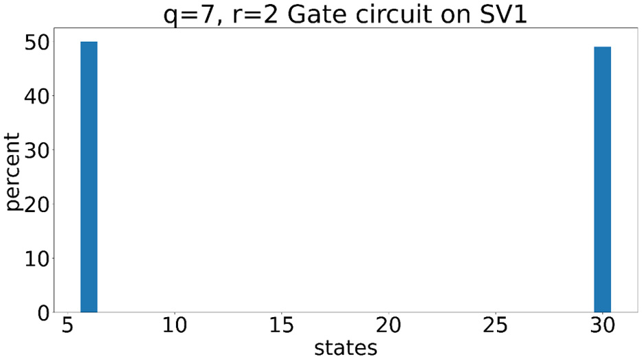
Figure 6.22 – Resulting state probabilities after using the gate circuit on SV1
- On TN1, we can only run the gate circuit. The following is the code and output from the TN1 execution:
- Assign the device:
device_name='TN1'
device=set_device(device_name)
estimate_cost(device)
Output:
Device('name': TN1, 'arn': arn:aws:braket:::device/quantum-simulator/amazon/tn1)
simulator cost per  minute : $ 0.275
total cost cannot be estimatedshots=estimate_cost_measured_qubits(device, n)
Output:
max shots: 1000
for 7 measured qubits the maximum allowed shots: 1,000
simulator cost per  minute : $ 0.275
total cost cannot be estimated
- Run the circuit:
title='q='+str(n)+', r='+str(r)+' Gate circuit on '+device_name
result=run_circuit(device, g_circ, shots, s3_folder, title, False)
Output:
6 : 49
30 : 50
The probabilities of the two states are also shown in the following bar chart:

Figure 6.23 – Resulting state probabilities after using the gate circuit on TN1
So far, we have seen that all these devices practically give the same results – at least, at the current number of qubits. This was intended to drive the point that all simulators should give the same values and that those values are consistent with matrix multiplication, which we learned about in this chapter.
In the next subsection, we will execute the same circuit, g_circ, on the IonQ device, as well as on the Rigetti Aspen M-1 device.
Execution on quantum devices
So far, we have executed the random circuit on simulators. Now, we will run it on quantum devices. We have access to IonQ, which has 11 qubits, and Rigetti’s Aspen M-1 quantum computer, which has 80 qubits. Of course, we will only use 7 qubits for this circuit. This process will give you a hands-on perspective regarding the performance of current quantum computers. Follow these steps:
Warning
Please only execute this section of the code if you are willing to be charged the cost of the quantum devices based on the number of shots submitted.
- First, we set must the device to IonQ Device. Next, we must estimate the number of shots based on the number of qubits that will be measured and then we run the circuit:
- Assign the device:
device_name='IonQ Device'
device=set_device(device_name)
estimate_cost(device)
Output:
Device('name': IonQ Device, 'arn': arn:aws:braket:::device/qpu/ionq/ionQdevice)
device cost per  shot : $ 0.01
total cost for 1000 shots is $10.30- Estimate the shots:
shots=estimate_cost_measured_qubits(device, n)
Output:
max shots: 10000
for 7 measured qubits the number of shots recommended: 3,200
device cost per  shot : $ 0.01
total cost for 3200 shots is $32.30
title='q='+str(n)+', r='+str(r)+
  ' Gate circuit on '+device_name
result=run_circuit(device, g_circ, shots, s3_folder,
                   title, False)
Output:
0 : 1
2 : 2
6 : 44
14 : 1
22 : 2
26 : 2
30 : 36
38 : 1
The following bar chart shows the results:
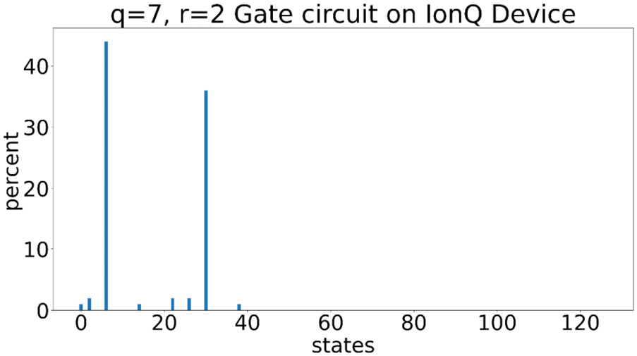
Figure 6.24 – Resulting state probabilities after running the gate circuit on the IonQ device
This is the first time we have seen other resulting values with small probabilities. It should be noted that the IonQ device has fully connected qubits and a reasonably low error rate. However, the probabilities of our two primary numbers have reduced to 44% and 36%, respectively. With more repetitions, these probabilities will reduce further due to errors arising in the execution of the gate operations.
Note – Using Native Gates to Improve Results
We have not used native gate operations for IonQ. Native gate operations are ideal for quantum computers. Single-qubit gate operations and especially two-qubit gate operations that use native gates have the least error. More information on this can be found in the Further reading section.
- Now, we will repeat the same steps on the available Rigetti Aspen device. Please run the available_devices() function to check which Aspen device is available. As of this writing both Aspen 11 and Aspen-M-1 quantum processors have been available at different times. Since Aspen has limited connectivity between qubits, it is important to set up the circuit with the architecture in mind. This will result in fewer errors in the output.
Note – Aspen M-1 Connectivity
The device.properties.dict()['paradigm']['connectivity'] function can be used to determine the connectivity between qubits.
The following code shows how to determine the Rigetti-M-1 quantum processor's connectivity and embed the quantum circuit on qubits that are connected:
- Assign the device:
device_name='Aspen-M-1'
device=set_device(device_name)
estimate_cost(device)
Output:
Device('name': Aspen-M-1, 'arn': arn:aws:braket:us-west-1::device/qpu/rigetti/Aspen-M-1)
device cost per  shot : $ 0.00035
total cost for 1000 shots is $0.65- Estimate the shots:
shots=estimate_cost_measured_qubits(device, n)
Output:
max shots: 100000
for 7 measured qubits the number of shots recommended: 3,200
device cost per  shot : $ 0.00035
total cost for 3200 shots is $1.42
device.properties.dict()['paradigm']['connectivity']
Output:
{'fullyConnected': False,
 'connectivityGraph': {'0': ['1', '103', '7'],
  '1': ['0', '16', '2'],
  '10': ['11', '113', '17'],
  '100': ['101', '107'],
  '101': ['100', '102', '116'],
  '102': ['101', '103', '115'],
  '103': ['0', '102', '104'],
…
  '2': ['1', '15'],
…
  '5': ['4', '6'],
  '6': ['5', '7'],
  '7': ['0', '6']}}
Based on this output, it appears that qubits 2 and 3 are not connected. The qubit connectivity appears to be as follows:
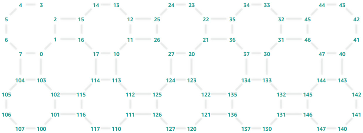
Figure 6.25 – Rigetti M-1 qubit connectivity
Since qubits 2 and 3 are not connected, the default embedding will use different qubit combinations and can result in a mapping we do not prefer. To hardcode the embedding, we will need to recreate the quantum circuit with the required qubit numbers.
- Rebuild the quantum circuit with the desired qubit mapping:
m=[10,11,12,13,14,15,16]
q=7
r=2
n=q
g_circ=Circuit().h([m[0],m[1],m[2],m[3],m[4],m[5],m[6]])
g_circ=g_circ.x(m[0]).i(m[1]).i(m[2]).t(m[3]).x(m[4]).x(m[5]).z(m[6])
g_circ=g_circ.i(m[0]).cnot(m[1],m[2]).cnot(m[3],m[4]).cnot(m[5],m[6])
g_circ=g_circ.x(m[0]).x(m[1]).x(m[2]).t(m[3]).x(m[4]).x(m[5]).z(m[6])
g_circ=g_circ.cnot(m[0],m[1]).cnot(m[2],m[3]).cnot(m[4],m[5]).i(m[6])
g_circ=g_circ.h([m[0],m[1],m[2],m[3],m[4],m[5],m[6]])
print(g_circ)
Output:
T   : |0|1|2|3|4|5|
q10 : -H-X-I-X-C-H-
               |
q11 : -H-I-C-X-X-H-
           |
q12 : -H-I-X-X-C-H-
               |
q13 : -H-T-C-T-X-H-
           |
q14 : -H-X-X-X-C-H-
               |
q15 : -H-X-C-X-X-H-
           |
q16 : -H-Z-X-Z-I-H-
T   : |0|1|2|3|4|5|
The preceding code creates the same random circuit we used on the simulators and IonQ. However, in this case, we are defining specific qubit numbers we want to use on the Rigetti Aspen M-1 device. This circuit is specifically for the Rigetti QPU as other devices do not allow us to skip qubit numbers. To enforce this embedding on the Rigetti device, we need to use the disable_qubit_rewiring=True parameter, as shown here:
result = device.run(circuit, shots=shots,
  s3_destination_folder=s3_folder,
   disable_qubit_rewiring=True).result()
Please review the run_rigetti() code to see how this is used. The rest of the code is the same as it is for run_circuit(). Let's proceed.
- Run the circuit:
title='q='+str(n)+', r='+str(r)+
  ' Gate circuit on '+device_name
result=run_rigetti(device, g_circ, shots, s3_folder,
                   title, False)
Output:
Device('name': Aspen-M-1, 'arn': arn:aws:braket:us-west-1::device/qpu/rigetti/Aspen-M-1)
0 : 1
2 : 2
4 : 1
6 : 11
10 : 1
14 : 4
22 : 1
24 : 1
26 : 2
30 : 11
38 : 3
46 : 2
54 : 1
58 : 1
62 : 5
70 : 1
94 : 1
98 : 1
102 : 5
110 : 2
118 : 2
120 : 1
122 : 1
126 : 5
The output values are in percent. As shown in the following chart, we have many more results showing up in the output with smaller probabilities:

Figure 6. 26 – Resulting state probabilities after running the gate circuit on the Rigetti Aspen-M-1 device
The probability of detecting the two primary numbers, 6 and 30, is now at 11%. Any more repetitions in this circuit and we would not be able to detect the expected output. Also, if we "carelessly" placed a circuit on the Aspen architecture and didn't try to carefully optimize the circuit to qubit connections, we would see more errors.
This exercise, along with the code samples and functions, should help you create sample quantum circuits or even build an equivalent unitary matrix using tensor products and matrix multiplication. The value will come from finding real use cases that require tensor products and then determining the equivalent gate model. The simulators can provide cost-effective ways of testing considerably large circuits. The Google Supremacy experiment is a great learning opportunity. You can try using different gates with random rotations as well, such as the RX, RY, and RZ gates. Many quantum gates are in the literature, and it is also important to review the gates that are available in the quantum devices. Gates such as xx, yy, and zz are available on IonQ and provide unique and flexible unitary matrices and qubit rotations to work with.
Summary
In this chapter, we looked at the basics of quantum gates and quantum circuits. Quantum circuits provide you with a unique opportunity to practice tensor products and work with complex numbers. We worked with simple matrices and showed how unitary matrices represent quantum gates. First, we experimented with a single-qubit system and looked at an example of encoding the time on a single qubit. Then, we learned how a quantum circuit with multiple qubits can be represented by tensor products and matrix multiplication, which leads to simulated results. Amazon Braket provides its own set of simulators that can take gate circuit instructions and provide the resulting probabilities. We saw that by using Amazon Braket simulators, it is possible to simulate considerably large circuits. Even though these classical resources take time, it will be advantageous to build up your skills to solve problems with these simulators while better quantum computers are developed that have been scaled up with more qubits and are less error-prone. We took our knowledge of developing a quantum circuit to build a random circuit inspired by the Google Supremacy experiment. We compared the results between our unitary matrix and those from the Amazon local simulator, the SV1 and TN1 simulators, and the IonQ and Rigetti AspenM-1 quantum computers.
Having gone over the basics of quantum circuits, in the next chapter, we will take the next step toward quantum algorithms.
Further reading
To learn more about the topics that were covered in this chapter, take a look at the following resources:
- Mathematics of quantum computing books by Packt Publishing:
- Essential Mathematics for Quantum Computing, by Leonard S. Woody III: https://www.packtpub.com/product/programming/9781801073141
- Dancing with Qubits, by Robert S. Sutor: https://www.packtpub.com/product/data/9781838827366
- Amazon Braket Documentation: https://docs.aws.amazon.com/braket/latest/developerguide
- Google Supremacy papers: https://www.nature.com/articles/s41586%20019%201666%205
- Response from IBM: https://www.ibm.com/blogs/research/2019/10/on-quantum-supremacy/
- NumPy functions:
- OpenQASM support in Amazon Braket:
- IonQ native gates:
- Rigetti native gates and qubit connectivity:
- Use the following code to find all supported gates:
device.properties.dict()['action']['braket.ir.jaqcd.program']['supportedOperations']
- Use the following code to find native gates:
device.properties.paradigm.nativeGateSet
- Use the following function to evaluate the connectivity:
device.properties.dict()['paradigm']['connectivity']
- Use the following setting to disable automated embedding of the circuit on qubits:
- disable_qubit_rewiring=True
Code deep dive:
Please review the code for the following functions, which were provided as part of the code for this chapter and can be found in this book’s GitHub repository:
- qc_rand()
- run_circuit()
- run_rigetti()