12

Multi-Objective Optimization Use Case

By now, you have gained the confidence to try various types of circuits, tests, and small problems on quantum computing and simulator devices available on Amazon Braket. You have learned how the annealer differs from gate quantum computers and the limits of each device. You have seen how to convert a constrained problem into a Quadratic Unconstrained Binary Optimization (QUBO) format. You have also learned how to develop a Binary Quadratic Model (BQM) to optimize the D-Wave annealer; the same BQM was used to create the quantum circuit for the QAOA algorithm for gate-based quantum computers. We used various matrices to represent a BQM and developed the BQM for the knapsack problem in the previous chapter.

In this final chapter, we will go over a scenario with two competing objectives. This will help you learn how to address real-world problems that have multiple and frequently conflicting objectives. We will look at a mock example of a retail store with two managers who have turned adversarial due to misaligned objectives and incentives based on their area performance.

First, we will develop the problem and then work through two scenarios. In one of the scenarios, a procurement manager is in control of prioritizing the objective and decides on which suppliers the company should work with. In the other scenario, an inventory manager, who works with marketing and the store managers, gets to decide which products are purchased. We will run these scenarios classically, then use the D-Wave annealer to analyze the current conflict. Then, we will find an optimal strategy that will benefit the whole store.

The following topics will be covered in this chapter:

• Looking into a mock inventory management problem
• Determining the conflict based on the opposing objectives
• Determining a better global solution

Technical requirements

The source code for this chapter is available in this book’s GitHub repository: https://github.com/PacktPublishing/Quantum-Computing-Experimentation-with-Amazon-Braket/tree/main/Chapter12.

Refreshed code utilizes D-Wave directly from D-Wave LEAP

Looking into a mock inventory management problem

We will start with a mock example to show how multiple and conflicting objectives can be evaluated and resolved using a simple method. We will follow these steps:

1. First, we will set up the multi-objective problem.
2. Then, we will show the two competing scenarios, A and B, in code.
3. Next, we will use the probabilistic solver we used in the previous chapter and find the optimal values using D-Wave through Amazon Braket.
4. Finally, we will find a method that finds the maximum benefit for both objectives.

Setting up the multi-objective problem

Let’s set up the problem. In this hypothetical scenario of a retail store, the inventory manager is accountable for stocking products that are in demand and generating the most revenue for the company by ensuring enough products are in stock. The procurement manager is responsible for ensuring that the products are procured with the least amount of risk and cost from reliable suppliers. The procurement manager wants to implement plans to reduce the overall risk. They wish to sign up the optimal number of key and reliable suppliers and factories without increasing any overhead and the additional risk of dealing with too many suppliers. This seems like a losing proposition when the product’s needs require signing up risky and high-cost suppliers.

The inventory manager has been trying to stock the right amount of products to meet the trends and demands of the customers, also ensuring complementary products are available and products with the least profit margin are not stocked. However, it seems like a losing battle, especially when the procurement manager cannot keep up with the product trends, and items that are not selling are bundled in with the shipments. The following diagram shows the current situation: we have product shortages and items that are not in demand stacking up in the inventory, as well as risky suppliers or others that seem to be fulfilling demand on schedule. Here, both the inventory and procurement managers are not achieving their target performance:

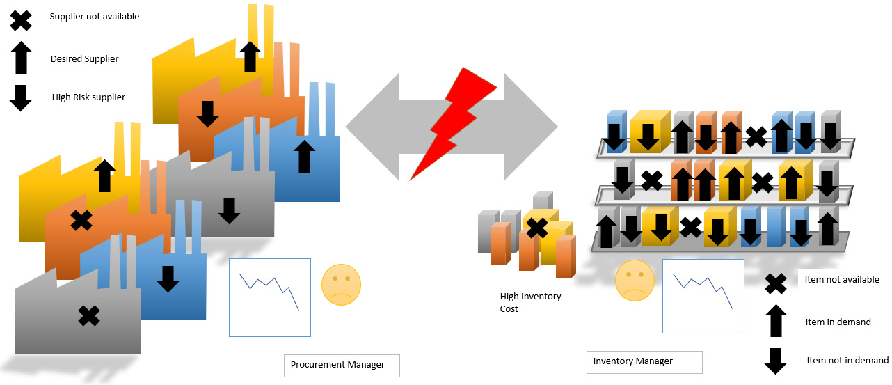
Figure 12.1 – Current situation between inventory and procurement

You have been assigned to help figure out how to resolve this situation. How can you help each manager optimize their area and, more importantly, can you find a solution to these competing objectives?

Let’s look at this problem systematically.

In Scenario A, we will do the following:

1. Optimize the suppliers based on the procurement manager’s data, which is stored in the Ms matrix.
2. Find the available items from those suppliers based on the availability matrix, Ma.
3. Create a new BQM for these new items and optimize the items for the inventory manager to place in the store.

In Scenario B, we will do the following:

1. Optimize the items based on the inventory manager’s data, which is stored in the Mi BQM matrix.
2. Find the minimum number of suppliers that can meet the item demand using the Ma matrix.

The following diagram shows a summary of how we want to optimize each scenario:

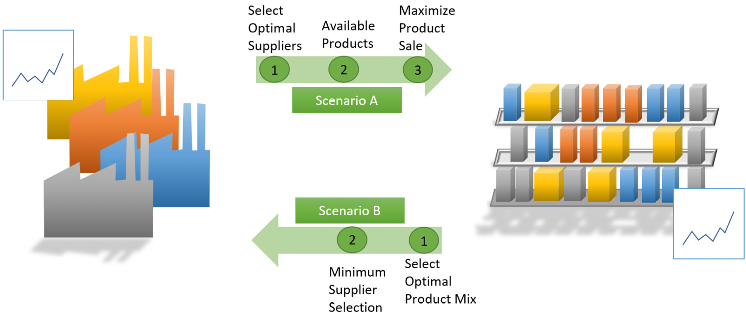
Figure 12.2 – Steps to evaluate the best solutions for scenarios A and B

In this mock example, we will assume that Ms is a matrix that represents the combined risk function of selecting a set of suppliers. We want to minimize the energy of this matrix for the procurement manager. A second matrix, Mi, represents the inventory energy function of the combination of items or products that are stocked. It has already been multiplied by -1, so we need to minimize the energy of this matrix. A third matrix, Ma, shows which products are available from each supplier. This matrix will be used in scenario A to find all the products available from the selected suppliers. It will also be used in scenario B to find the minimum suppliers that provide or cover the required items.

The following diagram shows the data in the availability matrix, Ma, and summarizes how it is used to achieve the goals of scenarios A and B:

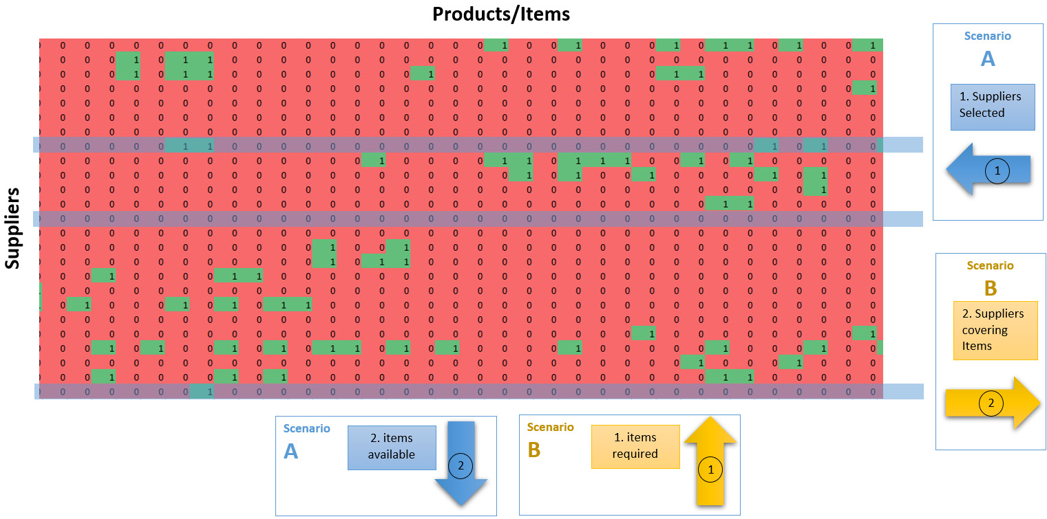
Figure 12.3 – The availability matrix, Ma, and its use in scenarios A and B

The key equations are given here:

These equations have the constraint that all items selected must be available at the selected suppliers.

Evaluating the best product mix based on scenario A

Now that we have set up the problem and know the two objectives and the constraint, let’s start reviewing the code to find the results of scenario A. In this case, we want to optimize using the supplier matrix, Ms, and then determine which products can be sold for maximum profit:

1. First, let’s import the three matrices that represent our problem – that is, Mi, Ms, and Ma:

   from numpy import genfromtxt
   Mi = genfromtxt('items.csv', delimiter=',')
   Ms = genfromtxt('supplier.csv', delimiter=',')
   Ma = genfromtxt('availability.csv', delimiter=',')
2. Next, we can review the shape and values of the three matrices. 80 items are represented in Mi:

   print(np.shape(Mi))
   print(Mi)

Output:

(80, 80)
[[-0.6   0.7   0.03 ...  0.02  0.01  0.03]
 [ 0.   -0.91  0.02 ...  0.03  0.04  0.  ]
 [ 0.    0.   -0.92 ...  0.01  0.02  0.04]
 ...
 [ 0.    0.    0.   ... -0.39  0.7   0.02]
 [ 0.    0.    0.   ...  0.    0.2  -0.9 ]
 [ 0.    0.    0.   ...  0.    0.   -0.34]]

This matrix is the standard upper triangular matrix we have used to represent a BQM. Negative values on the diagonal represent desired products and any negative non-diagonal terms represent complementary products that we want to select together. You may want to open and view the items.csv file for more details.

3. Let’s review the Ms matrix using the following code:

   print(np.shape(Ms))
   print(Ms)

Output:

(30, 30)
[[-1.30e+00  3.35e-02  4.91e-02  2.83e-02  1.03e-01  6.93e-02  7.03e-02
   3.57e-03  7.35e-02  1.19e-02  2.40e-02  1.14e-01  5.54e-02  8.98e-02
   1.08e-01  8.33e-02  1.99e-02  5.05e-03  3.46e-02  2.63e-02  1.90e-02
   7.09e-02  6.71e-02  1.02e-01  1.21e-01  7.46e-02  1.22e-01  8.05e-02
   2.03e-02  3.35e-02]
 …
[ 0.00e+00  0.00e+00  0.00e+00  0.00e+00  0.00e+00  0.00e+00  0.00e+00
   0.00e+00  0.00e+00  0.00e+00  0.00e+00  0.00e+00  0.00e+00  0.00e+00
   0.00e+00  0.00e+00  0.00e+00  0.00e+00  0.00e+00  0.00e+00  0.00e+00
   0.00e+00  0.00e+00  0.00e+00  0.00e+00  0.00e+00  0.00e+00  0.00e+00
   0.00e+00 -4.06e-01]]

The Ms matrix is also a BQM that represents 30 suppliers.

4. Now, let’s review the Ma matrix, which contains the item availability information:

   print(np.shape(Ma))
   print(Ma)

Output:

(30, 80)
[[0. 0. 0. ... 0. 0. 0.]
 [0. 1. 0. ... 1. 0. 0.]
 [0. 0. 0. ... 0. 0. 0.]
 ...
 [1. 0. 0. ... 0. 0. 0.]
 [1. 0. 1. ... 0. 0. 0.]
 [0. 0. 0. ... 0. 0. 0.]]

The Ma matrix represents item availability and is displayed in the preceding output. Notice that the matrix is not the standard BQM. This matrix is a 30x80 matrix. The 30 rows represent the 30 suppliers, while the 80 rows represent the 80 items. A 1 indicates that the item is available at the supplier.

5. We can quickly visualize the Ms matrix by using the probabilisticsampler() function:

   sup_list=ProbabilisticSampler(Ms,100)

Output:

Best found: [0, 1, 5, 6, 10, 12, 14, 20, 26, 29]
count: 10
Energy: -8.9079
Solutions Sampled: 2762

With only 100 samples per number of suppliers in the solution, we find that the best supplier combination is [0, 1, 5, 6, 10, 12, 14, 20, 26, 29]. This is 10 suppliers with the lowest energy of -8.9079. This would recommend that the procurement manager only signs contracts with these suppliers. Since this is a probabilistic result, your execution may produce slightly different values. The following plot shows that there are other likely minimum values between 10 and 14 suppliers. It also shows that there is a broad range of energy values for those supplier numbers, indicating that picking the wrong 10 suppliers could have a large impact on the risk of supplier selection:

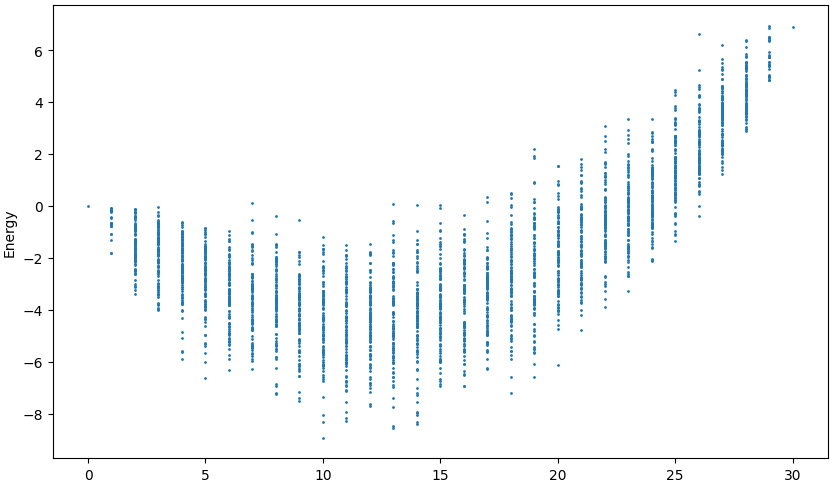
Figure 12.4 – Supplier BQM matrix, Ms, energy landscape visualization

6. Now, we want to see which items are available through these suppliers. Let’s use the availability() function to get a list of available items for a list of suppliers while using the Ma matrix:

   a=availability(sup_list[0],Ma)
7. We can review the list of available items, a, from all these suppliers using the following command:

   print(len(a),a)

Output:

43 [ 0  1  2  3  5  9 14 16 17 22 24 25 28 29 32 35 36 38 39 41 42 44 45 46
 47 48 50 51 52 53 54 55 57 58 60 63 65 66 69 70 74 76 77]

Based on the selected suppliers, the output shows that there are 43 available items that the inventory manager can now decide to stock in the store. Since this is a probabilistic result, your execution may produce slightly different values.

8. The inventory manager does not want to stock all items; they would prefer to optimize within the available items to see which would be the most optimal in reducing costs and maximizing profit. To do this, we need to provide the inventory manager with a new BQM matrix that represents these items only. The item_m() function has been provided for this. In this case, the list, a, represents the items available based on the optimal suppliers, and Mi is the inventory BQM for all items. The resulting m_i is a smaller subset BQM matrix of the new items available to the inventory manager:

   m_i=item_m(a, Mi)
   print(np.shape(m_i))
   print(m_i)

Output:

(43, 43)
[[-0.6   0.7   0.03 ...  0.    0.02  0.02]
 [ 0.   -0.91  0.02 ...  0.04  0.    0.03]
 [ 0.    0.   -0.92 ...  0.03  0.02  0.01]
 ...
 [ 0.    0.    0.   ... -0.93  0.03  0.02]
 [ 0.    0.    0.   ...  0.    0.02 -0.9 ]
 [ 0.    0.    0.   ...  0.    0.   -0.39]]

The preceding matrix represents the BQM for the 43 items that are now available to the inventory manager. Now, we can simply optimize this matrix to find the optimal items to stock.

9. Let’s use the ProbabilisticSampler() function once more to evaluate the optimal products:

   p_items=ProbabilisticSampler(m_i,100)

Output:

Best found: [1, 2, 4, 5, 6, 7, 8, 10, 11, 12, 13, 15, 16, 18, 20, 21, 23, 28, 29, 31, 32, 33, 35, 36, 37, 38, 39, 40]
count: 28
Energy: -14.850000000000051
Solutions Sampled: 4088

Out of the 43 items, the inventory manager will now stock only 28 items, as shown in the preceding output. Keep in mind that the index values for these 28 items are based on the new m_i matrix and that to retrieve the actual product number, we will have to refer to the original indexes in the Mi matrix. This is not necessary right now and will be shown in the next section. The main point so far is that this gives a minimum energy value of -14.85 for the inventory. The visualization of the m_i matrix is given in the following plot. Would the inventory manager be happy with this option?

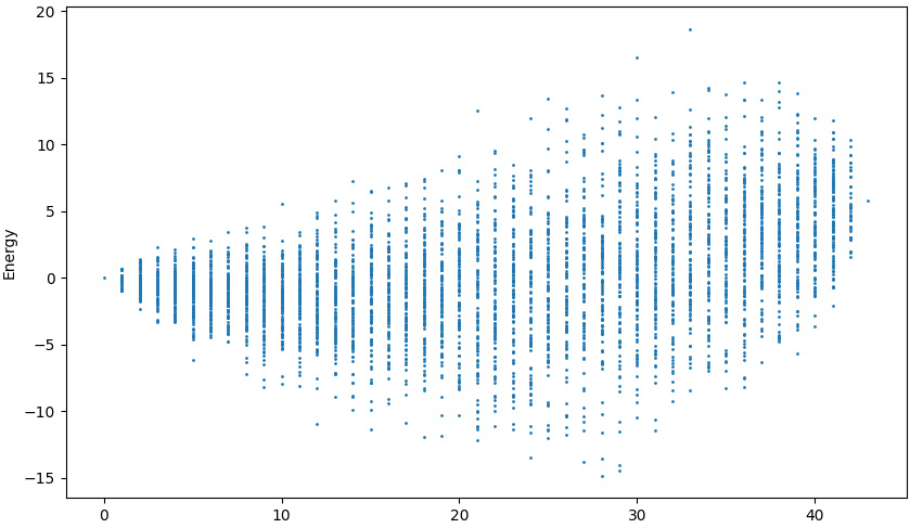
Figure 12.5 – Available inventory BQM matrix, m_i, energy landscape visualization

So far, we have looked at the initial steps and process of how to optimize the suppliers and then the inventory. With our classical probabilistic sampler and with just a few shots, we found that the procurement manager could get an energy value of -8.9079 with 10 suppliers. Then, we evaluated the available items from these combined sets of suppliers to determine that the optimal set of products to be stocked was 28 with an energy value of -14.85. However, this was just the beginning; we want to find better values for both managers, run through scenario A, and then work backward from the inventory to the supplier optimization in scenario B. We will go over this next.

Determining the conflict based on the opposing objectives

Now, we want to loop through the steps in the previous section to find better results for scenario A and then work backward to find reasonably good values for scenario B. Please refer to Figure 12.2, which summarizes these steps. First, we will do this with the classical probabilistic solver and then use D-Wave.

Evaluating the results with the probabilistic solver

We can quickly visualize and then evaluate the conflict by looping through the steps multiple times and plotting the results of each scenario. Here, we will continue to use the probabilistic solver:

1. The following code is for scenario A and accumulates supplier and inventory energy values for plotting. We will repeat the process 20 times, as set in the total variable. The code lines should be familiar from the previous section. At the end of the code, we will convert the item values from the m_i matrix into actual product numbers that are stored in i_item. The energy values from the supplier list are stored in plot_sup1, while the energy values from the resulting inventory in p_items are stored in plot_prod1. We will start by finding the optimal suppliers and then finding the items that are available from those suppliers. We will only show the results of the first iteration:

   plot_sup1=[]
   plot_prod1=[]
   total=20
   for trials in range(total):
       sup_list=ProbabilisticSampler(Ms,100)
       print('Ideal suppliers:',sup_list[0])
       print('Supplier energy', sup_list[1])
   # save the energy of the best suppliers for plotting
       plot_sup1.append(sup_list[1])
   # calculate list of available items
       a=availability(sup_list[0],Ma)
       print('Items available:',len(a),a)
   # build new BQM of the available items
       m_i=item_m(a, Mi)
       print(np.shape(m_i))

Output:

Best found: [0, 5, 10, 11, 12, 14, 15, 20, 21]
count: 9
Energy: -9.184190000000001
Solutions Sampled: 2762
Ideal suppliers: [0, 5, 10, 11, 12, 14, 15, 20, 21]
Supplier energy -9.184190000000001
Items available: 40 [ 0  2  3  5  8  9 13 15 18 20 22 23 24 25 27 29 32 35 36 38 39 41 42 44
 45 46 47 48 50 51 52 53 54 55 66 69 70 74 77 79]
(40, 40)

The preceding output is only for the first output of 20. The plots of the energy landscape are available in this book's GitHub repository for this chapter and have not been shown here. These plots of the energy landscape of the Ms matrix will be similar to those in Figure 12.4. This output shows that 9 suppliers were selected, which resulted in a total of 40 items becoming available to the inventory manager. The supplier energy value was -9.18.

2. Next, we will optimize the items that should be stocked in the store by the inventory manager:

   # find optimal items to stock in store
       p_items=ProbabilisticSampler(m_i,100)
   # refer back to original item numbers in Mi
       i_item=np.zeros(len(p_items[0]))
       for I in range(len(p_items[0])):
           i_item[i]=a[p_items[0][i]]
       print('Items in solution:',i_item)
       print('Item Energy', p_items[1])
   # store the energy of the optimal items for plotting
       plot_prod1.append(p_items[1])

Output:

Best found: [1, 2, 3, 5, 6, 7, 9, 10, 11, 12, 13, 14, 19, 20, 23, 25, 27, 29, 30, 31, 32, 33, 34, 35, 36, 37, 38, 39]
count: 28
Energy: -17.940000000000083
Solutions Sampled: 3781
Items in solution: [ 2.  3.  5.  9. 13. 15. 20. 22. 23. 24. 25. 27. 38. 39. 44. 46. 48. 51.
 52. 53. 54. 55. 66. 69. 70. 74. 77. 79.]
Item Energy -17.940000000000083

In this case, we have 28 optimal items, with an energy value of -17.94. The plot of the energy landscape for the m_i matrix has not been shown here but it will be similar to what's shown in Figure 12.5. Also, note that we converted the item numbers from the optimized list back into the original index of the items in the Mi matrix.

3. The following code is for scenario B and accumulates supplier and inventory energy values for plotting. We will perform the steps for scenario B 20 times as well. Please refer to Figure 12.2 for the key steps in scenario B. In this case, we will find the optimal items from all 80 items in the Mi BQM matrix. Next, we will use a new function, SetCoverSampler(), to find the minimum suppliers that provide those items. This new function is a modification of the probabilistic sampler so that we can visualize the energy landscape. More efficient code can be created for this purpose as well if desired. A plot of the first iteration is shown in Figure 12.6. Then, we will find the energy value of these suppliers from the Ms BQM matrix. We won’t need to optimize any further since the set cover means that the minimum suppliers have been found. Finally, all the energy values will be stored for plotting.

Let's proceed with the code for these two steps for scenario B. First, we will find the optimal items using the Mi BQM matrix:

plot_sup2=[]
plot_prod2=[]
total=20
for trials in range(total):
# optimize and print energy landscape for Mi
    p_items=ProbabilisticSampler(Mi,100)
    print('Ideal items:', p_items[0])
    print('Items energy:', p_items[1])
# store energy of items for plotting 
    plot_prod2.append(p_items[1])

Output:

Best found: [1, 4, 5, 7, 9, 10, 11, 13, 15, 24, 26, 27, 33, 34, 37, 38, 39, 40, 44, 45, 47, 49, 50, 52, 56, 57, 58, 63, 64, 65, 66, 69, 71, 72, 73, 75, 77, 78, 79]
count: 39
Energy: -36.94999999999979
Solutions Sampled: 7862
Ideal items: [1, 4, 5, 7, 9, 10, 11, 13, 15, 24, 26, 27, 33, 34, 37, 38, 39, 40, 44, 45, 47, 49, 50, 52, 56, 57, 58, 63, 64, 65, 66, 69, 71, 72, 73, 75, 77, 78, 79]
Items energy: -36.94999999999979

Please review the output in the code in this chapter's GitHub repository. The output shows that 39 optimum items were found from the total of 80 items for stocking in the store. The energy value of these items is -36.94 and has been saved for plotting.

4. Next, we will use the SetCoverSampler() function to find the minimum suppliers that provide those items. This new function is a modification of the probabilistic sampler so that we can visualize the energy landscape. More efficient code can be created for this purpose as well if desired:

   # find energy landscape for set cover and minimum 
   # suppliers to cover required items
       sup_list=SetCoverSampler(Ma,p_items[0],100)
       print('Min Suppliers to cover items:',sup_list[0])

Output:

Best found: [0, 1, 2, 4, 8, 9, 10, 12, 14, 15, 17, 18, 20, 21, 22, 23, 24, 25, 26, 27, 28]
count: 21
Energy: -39.0
Solutions Sampled: 2762
Min Suppliers to cover items: [0, 1, 2, 4, 8, 9, 10, 12, 14, 15, 17, 18, 20, 21, 22, 23, 24, 25, 26, 27, 28]

In the output, we find 21 suppliers that cover the 39 required items.

A plot of the first iteration is shown here. You can see that the energy drops as the number of suppliers increases. This shows that more items are being covered by the increasing number of suppliers. At 21 suppliers (X-axis), the minimum energy is found and all the items are covered. This energy value of -39 represents the solution covering the 39 items. As we increase the suppliers, the value is not improved. We only need to return the lowest number of suppliers where the lowest energy is found:

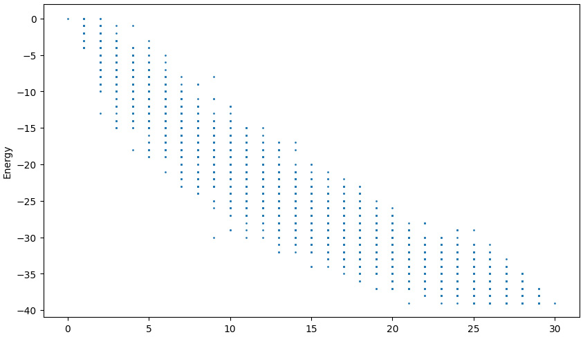
Figure 12.6 – Supplier energy landscape from the SetCoverSampler() function

5. Now, we must simply find the energy of the suppliers based on the data in the Ms matrix and also store the energy for plotting:

   # Find the minimum suppliers that cover required items
       sup_list=SetCoverSampler(Ma,p_items[0],100)
       sup_energy=0
       for i in sup_list[0]:
           for j in sup_list[0]:
               if i<=j:
                   sup_energy+=Ms[i,j]
       print('Supplier Energy',sup_energy)
   # save minimum supplier energy for plotting
       plot_sup2.append(sup_energy)

Output:

Supplier Energy -0.3361099999999987

6. Now, we can plot the results:

   plt.scatter(plot_sup1,plot_prod1,color='green')
   plt.scatter(plot_sup2,plot_prod2,color='red')
   plt.xlabel('supplier')
   plt.ylabel('product')
   plt.title('Find optimal supplier and product')

The resulting plot is as follows:

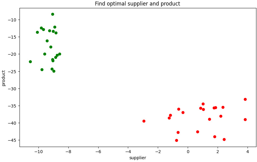
Figure 12.7 – Results from sampling scenario A (top left green dots) and scenario B (bottom right red dots)

As you can see, with these quick classical results, the two objectives – supplier optimization and product optimization – conflict. In the plot data for scenario A (top left green dots), the supplier energy value is low, making the procurement manager happy. However, the product energy value is not optimized based on the available items. On the other hand, as shown in the plot data for scenario B (bottom right red dots), the inventory manager will get good results due to the low product energy value. However, the supplier energy value is not optimized. In the latter case, the procurement manager, by providing the required items, is not able to optimize the suppliers.

If the corporation is evaluating each manager for their specific performance and compensating them for optimizing their area, this will result in an internal conflict. These misaligned objectives will cause an adversarial relationship between the managers and the haphazard scenario shown in Figure 12.1.

We now have a general picture of the situation. Since the classical method requires a considerable amount of time to visualize the landscape, we sampled a limited number of times, so we did not get the best value for each scenario. In the next section, we will use D-Wave to find the optimal (or close to optimal) values for both scenarios.

Evaluating the optimal values using the D-Wave annealer

The plots in the previous section showed considerable variance. Depending on the suppliers selected, many item combinations are possible and depending on the items selected, many different supplier combinations are possible. Now, let’s turn to the D-Wave annealer to give us the best energy values possible for the two scenarios:

1. Starting with scenario A, we will optimize the suppliers using the Ms BQM matrix. We will use the run_dwave() function to find the optimal value for this matrix. We will use a value of 0.5 for the chain strength as a starting point. This can be changed to find possibly better solutions considering the number of variables. The run_dwave() function is set up to use the D-Wave Advantage system, which can embed a fully connected matrix whose size does not exceed 134. Since our matrix size was 110, we cannot use D-Wave 2000Q, which only has a capacity for embedding a fully connected matrix that’s 65 in size. Let's proceed:

   dwave_plot_sup1=[]
   dwave_plot_prod1=[]
   sup_result=run_dwave(Ms,0.5)

Output:

Number of qubits:  5760
Number of couplers 40135
Shots max 10,000
26843545600
Recommended shots 10000
Estimated cost $2.20
      0  1  2  3  4  5  6  ... 29     energy num_oc. ...
0     1  0  0  0  0  1  1  ...  0  -11.68817      68 ...
1492  1  0  0  0  0  1  1  ...  0  -11.68817       1 ...
['BINARY', 5022 rows, 10000 samples, 30 variables]
{0: 1, 1: 0, 2: 0, 3: 0, 4: 0, 5: 1, 6: 1, 7: 1, 8: 1, 9: 1, 10: 1, 11: 1, 12: 0, 13: 0, 14: 1, 15: 0, 16: 0, 17: 0, 18: 0, 19: 0, 20: 1, 21: 1, 22: 0, 23: 0, 24: 0, 25: 0, 26: 0, 27: 0, 28: 1, 29: 0}
100001111111001000001100000010
decimal equivalent: 570196738
Validate energy -11.688170000000005

We will process this data and clean it up in the next line.

2. Now, let's process the output to get the suppliers and energy values:

   first_sup=sup_result.first    
   sup_list=[]
   for s in range(len(Ms)):
       if first_sup.sample[s]==1:
           sup_list.append(s)
   print(sup_list)
   print('Supplier energy', first_sup[1])
   dwave_plot_sup1.append(first_sup[1])

Output:

[0, 5, 6, 7, 8, 9, 10, 11, 14, 20, 21, 28]
Supplier energy -11.688170000000003

Already, we can see that this energy value is the lowest we have seen for the suppliers.

3. Now, we need to find the items that are available based on this reduced supplier list:

   a=availability(sup_list,Ma)
   print('Items available:',len(a),a)

Output:

Items available: 54 [ 0  1  2  3  5  8  9 13 15 16 17 18 20 22 23 24 25 27 29 30 31 32 33 34 35 36 37 38 39 40 41 42 44 45 46 47 48 49 50 51 52 53 55 57 58 66 69 70 74 75 76 77 78 79]

4. Now, we must optimize these items since we've created a BQM matrix for them:

   m_i=item_m(a, Mi)
   print(np.shape(m_i))
   item_result=run_dwave(m_i,0.5)

Output:

(54, 54)
Number of qubits:  5760
Number of couplers 40279
Shots max 10,000
450359962737049600
Recommended shots 10000
Estimated cost $2.20
      0  1  2  3  4  5  6  7  ... 53 energy num_oc. ...
0     0  1  1  1  1  1  1  1  ...  1 -38.97      36 ...
2     0  1  1  1  1  1  1  1  ...  1 -38.97      31 ...

5. Now, we must extract the items from the D-Wave solution, calculate the energy of these items based on the new m_i matrix, and remap them to their original index:

   first_item=item_result.first
   itm_list=[]
   for s in range(len(m_i)):
       if first_item.sample[s]==1:
           itm_list.append(s)
   i_item=np.zeros(len(itm_list))
   for i in range(len(itm_list)):
       i_item[i]=a[itm_list[i]]
   print('Items in solution:',i_item)
   print('Item Energy:', first_item[1])
   dwave_plot_prod1.append(first_item[1])

Output:

Items in solution: [ 1.  2.  3.  5.  8.  9. 13. 15. 23. 25. 34. 37. 38. 39. 40. 42. 44. 53. 57. 58. 69. 70. 74. 75. 77. 78. 79.]
Item Energy: -38.969999999999885

Interestingly, this energy value is the best we have seen for the inventory. Should the inventory manager accept this solution? Let's continue to find out.

6. Here is the code for plotting this new result (purple) on the previous plot:

   plt.scatter(dwave_plot_sup1,dwave_plot_prod1,
               color='purple')
   plt.scatter(plot_sup1,plot_prod1,color='green')
   plt.scatter(plot_sup2,plot_prod2,color='red')
   plt.xlabel('supplier')
   plt.ylabel('product')
   plt.title('Find optimal supplier and product')

This results in the following output:

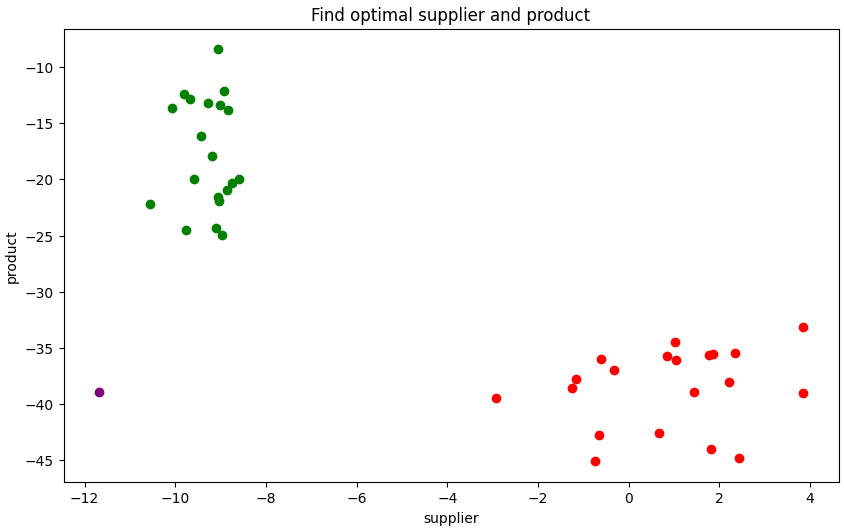
Figure 12.8 – Additional plot of the D-Wave results for scenario A (a single purple dot at the bottom left)

These are excellent results for the procurement manager, and to some extent, they are not too bad for the inventory manager. However, we have not seen how much better the inventory manager can do if using D-Wave to find the optimal results from scenario B.

7. We will now reverse the process for scenario B. In this case, we will start by optimizing the inventory using D-Wave:

   dwave_plot_sup2=[]
   dwave_plot_prod2=[]
   item_results=run_dwave(Mi,0.5)

Output:

Shots max 10,000
30223145490365729367654400
Recommended shots 10000
Estimated cost $2.20
      0  1  2  3  4  5  6  7  ... 79 energy num_oc. ...
13    0  0  1  1  1  1  1  1  ...  1 -90.39       8 ...

This is quite an unexpected result. The inventory manager has the option of getting an energy value of -90.39 based on the correct selection of items based on the Mi BQM matrix.

8. Now, we need to extract the item values and then process them to see which suppliers provide these items:

   first_item=item_results.first
   itm_list=[]
   for s in range(len(Mi)):
       if first_item.sample[s]==1:
           itm_list.append(s)
   print('items:',itm_list)
   print('Supplier energy', first_item[1])
   dwave_plot_prod2.append(first_item[1])

Output:

items: [2, 3, 4, 5, 6, 7, 8, 9, 10, 11, 12, 13, 14, 15, 19, 25, 26, 34, 37, 38, 39, 40, 41, 42, 43, 44, 46, 50, 52, 53, 55, 56, 57, 58, 59, 62, 63, 69, 70, 71, 72, 73, 74, 75, 76, 77, 78, 79]
Supplier energy -90.38999999999956

9. We will still use the probabilistic SetCoverSampler() function to determine the minimum suppliers needed to cover these items:

   sup_list=SetCoverSampler(Ma,itm_list,50)

Output:

Best found: [0, 1, 2, 3, 4, 6, 7, 8, 9, 13, 14, 15, 16, 17, 18, 20, 21, 23, 24, 26, 27, 29]
count: 22
Energy: -47.0
Solutions Sampled: 141

10. Now, we need to find the actual supplier energy for this mix of 22 suppliers:

    print('Min Suppliers to cover items:',sup_list[0])
    sup_energy=0
    for i in sup_list[0]:
        for j in sup_list[0]:
            if i<=j:
                sup_energy+=Ms[i,j]
    print('Supplier Energy',sup_energy)
    dwave_plot_sup2.append(sup_energy)

Output:

Min Suppliers to cover items: [0, 1, 2, 3, 4, 6, 7, 8, 9, 13, 14, 15, 16, 17, 18, 20, 21, 23, 24, 26, 27, 29]
Supplier Energy -0.16731999999999692

This energy value for the suppliers is quite poor. The considerable improvement in the product energy value has resulted in a very poor outcome for the supplier risks energy value. This result is not going to please the procurement manager.

11. Now, let’s plot these results and relook at the energy value comparison of the two scenarios:

    plt.scatter(dwave_plot_sup1,dwave_plot_prod1,color='black')
    plt.scatter(dwave_plot_sup2,dwave_plot_prod2,color='red')
    plt.scatter(plot_sup1,plot_prod1,color='gray')
    plt.scatter(plot_sup2,plot_prod2,color='pink')
                
    plt.xlabel('supplier')
    plt.ylabel('product')
    plt.title('Find optimal supplier and product')

The results are shown in the following plot:

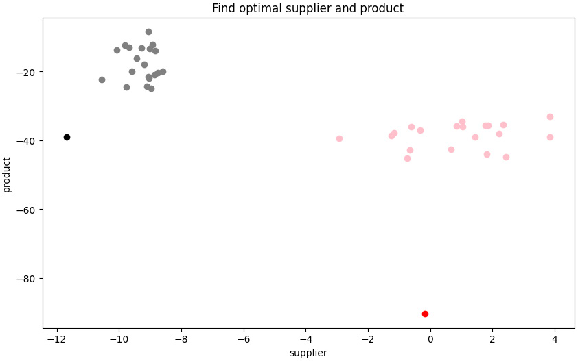
Figure 12.9 – Classical and D-Wave results for scenario A (left) and B (right)

The ideal scenarios for each area are detrimental to the other area. The procurement manager has been working toward pushing the risks lower toward the D-Wave result (the single purple dot on the left of the plot), while the inventory manager has been driving toward the best overall inventory outcome, as shown by the D-Wave result (the single red dot at the bottom right of the plot). Both these efforts hurt the other area and if compensation is misaligned, the conflict will remain.

With that, we have seen how the two objectives force the company in two different directions. These types of multi-objective scenarios exist when the dynamics within a company aren’t understood completely. Now, it’s time to determine how our quantum annealing method can find a resolution to this dilemma.

Determining a better global solution

How can we address both objectives and find a global solution? A mathematical treatment of creating a QUBO that represents both objectives and includes the appropriate constraint with a set cover formulation is outside the scope of this book. Please check out the Further reading section for examples and more details regarding this area. However, we can use a simple method with the techniques we have developed to find an answer.

Here are the high-level steps we will go over:

1. Create a combined BQM matrix, Mf, with both the Ms and Mi matrices and find an appropriate way to "connect" the items to the suppliers using Ma. We are looking for a way where, if an item is picked in the solution, there is a large negative coupling value that will also cause the optimization to pick the appropriate supplier of that item (and vice versa). We will use a multiplier, A, that is large enough to ensure this condition is enforced:

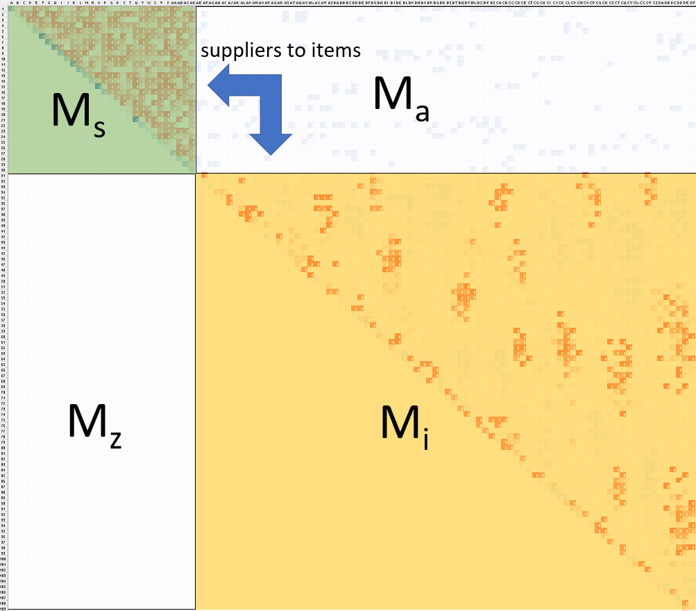
Figure 12.10 – Combined BQM matrix, Mf

2. Since the supplier units are not the same as the item units, we will combine them into one objective, along with the I and S multipliers, which we can use to change the relative strength of the values of Mi and Ms, respectively.
3. This method is not guaranteed to ensure valid solutions are found. We will have to extract the values of the suppliers and items and then validate if the solution is feasible based on the Ma availability matrix. We can only influence that the correct items and supplier combinations are picked by adjusting the value of A.
4. We will plot both the infeasible and feasible solutions that are found on the same plot.
5. We will also span through various multiplier values – A, I, and S – to find where the best feasible solutions are found. We will save various feasible solutions from different trials and then plot the results.
6. Finally, we will plot the values found with the highest product of the supplier and inventory energy values. This will give us a final set of the most optimal solutions.

With that, we have summarized the steps needed to find the global solution to the two conflicting objectives. In the next section, we will implement this in code.

Evaluating with the classical probabilistic solver

Let’s get started and learn how to implement the high-level steps mentioned earlier using the classical probabilistic solver method:

1. First, we will set the multipliers and create the modified Ma matrix, Ma2. Here, if an item is provided by a supplier, we will replace 1 in the matrix with -A. This way, we can change the strength of A to enforce this constraint:

   A=0.5
   S=2.5
   I=0.5
   Ma2=Ma.copy()
   Ma2 = np.where(Ma2==1, -A, 0)
   print(Ma2)
   print(np.shape(Ma2))

Output:

[[ 0.   0.   0.  ...  0.   0.   0. ]
 [ 0.  -0.5  0.  ... -0.5  0.   0. ]
 [ 0.   0.   0.  ...  0.   0.   0. ]
 ...
 [-0.5  0.   0.  ...  0.   0.   0. ]
 [-0.5  0.  -0.5 ...  0.   0.   0. ]
 [ 0.   0.   0.  ...  0.   0.   0. ]]
(30, 80)

If A is too large, it will overshadow the effects of the Mf and Mi matrices, while if A=0, the optimization will lead to all items and suppliers, which is not feasible.

2. Now, we can stitch together the Mf matrix, as shown in Figure 12.10:

   Mz=np.zeros([len(Mi),len(Ms)],dtype=float)
   print('Mz',np.shape(Mz))
   Msz=np.append(S*Ms, Mz, axis=0)
   print('Msz',np.shape(Msz))
   Mai=np.append(Ma2, I*Mi, axis=0)
   print('Mai',np.shape(Mai))
   Mf=np.append(Msz,Mai, axis=1)
   print('Mf',np.shape(Mf))
   print(Mf)
   np.savetxt('Mf.csv', Mf, delimiter=',')

Output:

Mz (80, 30)
Msz (110, 30)
Mai (110, 80)
Mf (110, 110)
[[-3.25     0.08375  0.12275 ...  0.       0.       0.     ]
 [ 0.      -0.415    0.23575 ... -0.5      0.       0.     ]
 [ 0.       0.      -0.365   ...  0.       0.       0.     ]
 ...
 [ 0.       0.       0.      ... -0.195    0.35     0.01   ]
 [ 0.       0.       0.      ...  0.       0.1     -0.45   ]
 [ 0.       0.       0.      ...  0.       0.      -0.17   ]]

The shape of the new Mf matrix is 110x110 and has been saved to the Mf.csv file.

3. Since this is a valid BQM matrix, we can quickly check it using the probabilistic solver:

   result=ProbabilisticSampler(Mf,100) 

Output:

Best found: [0, 1, 4, 5, 6, 7, 8, 9, 10, 11, 13, 14, 15, 16, 17, 18, 20, 21, 22, 23, 24, 26, 27, 28, 29, 30, 32, 33, 34, 35, 36, 37, 38, 39, 40, 41, 42, 43, 44, 45, 47, 48, 49, 50, 51, 52, 53, 54, 55, 58, 60, 61, 62, 63, 64, 66, 67, 68, 69, 70, 71, 72, 73, 75, 76, 77, 78, 79, 80, 82, 83, 84, 85, 86, 87, 88, 89, 90, 91, 92, 93, 94, 95, 97, 98, 99, 100, 101, 103, 104, 105, 106, 107, 108, 109]
count: 95
Energy: -80.00992500000018
Solutions Sampled: 10902

What do all these values mean? The resulting index values represent both the supplier and item values. The values from 0 to 29 represent the 30 suppliers, while the values from 30 to 109 represent the 80 items. The energy value of -80.00 does not correspond to the supplier or item energy, but that of the overall optimal for the full Mf matrix. Thus, we have to ensure that this is a feasible solution and then separately calculate the supplier and inventory energy values.

4. We can extract the supplier and item values using the following code:

   sup_list=[]
   item_list=[]
   for i in (result[0]):
       if i<len(Ms):
           sup_list.append(i)
       else:
           item_list.append(i-len(Ms))
5. Now, let’s print the lists and calculate the supplier and item energies:

   print(sup_list)
   sup_energy=0
   for i in sup_list:
       for j in sup_list:
           if i<=j:
               sup_energy+=Ms[i,j]
   print('Supplier Energy',sup_energy)
   print(item_list)
   item_energy=0
   for i in item_list:
       for j in item_list:
           if i<=j:
               item_energy+=Mi[i,j]
   print('Item Energy',item_energy)

Output:

[0, 1, 4, 5, 6, 7, 8, 9, 10, 11, 13, 14, 15, 16, 17, 18, 20, 21, 22, 23, 24, 26, 27, 28, 29]
Supplier Energy -1.1539699999999968
[0, 2, 3, 4, 5, 6, 7, 8, 9, 10, 11, 12, 13, 14, 15, 17, 18, 19, 20, 21, 22, 23, 24, 25, 28, 30, 31, 32, 33, 34, 36, 37, 38, 39, 40, 41, 42, 43, 45, 46, 47, 48, 49, 50, 52, 53, 54, 55, 56, 57, 58, 59, 60, 61, 62, 63, 64, 65, 67, 68, 69, 70, 71, 73, 74, 75, 76, 77, 78, 79]
Item Energy -10.249999999999492

6. The following code checks if a feasible solution has been found. First, we will extract the available items, a, based on the suppliers in the solution. Next, we will check if each of the items in the solution are included in the available item list. If all the selected items are found in the selected supplier, then the condition is met, and we have a feasible solution. On the other hand, if even one item in the solution is not found in the available item list, this means the solution cannot be feasible. Let’s print out the condition array so that you can check the status of each item:

   a=availability(sup_list,Ma)
   print('all items available',a)
   # Is this feasible:
   if(np.isin(False,(np.isin(item_list,a)))):
       print('Not feasible')
   # print result of each condition
       print(np.isin(item_list,a))
   else:
       print('Feasible')

Output:

all items available [ 0  1  2  3  4  5  6  7  8  9 10 11 12 13 14 15 16 17 18 19 20 21 22 23
 24 25 27 28 29 30 31 32 33 34 35 36 37 38 39 40 41 42 44 45 46 47 48 49
 50 51 52 53 55 56 57 58 59 60 62 63 64 65 66 68 69 70 71 72 73 74 75 76
 77 78 79]
Not feasible
[ True  True  True  True  True  True  True  True  True True  True  True  True  True  True  True  True  True  True  True  True  True  True  True  True  True  True  True  True  True  True  True  True  True  True  True  True False  True  True  True  True  True  True  True  True False  True  True  True  True  True  True False  True  True  True  True False  True  True  True  True  True  True  True  True  True  True  True]

In this example, we found an infeasible solution because a few of the items in the solution were not in the available item list. We want to repeat this process many times so that we can accumulate several optimal solutions and separate the feasible solutions from the infeasible ones. Rather than using the probabilistic sampler, we will use the strength of the D-Wave device and its ability to find many good solutions.

Evaluating the best solution using D-Wave

In the previous section, we used fixed values of S, I, and A. It turns out that we did not get a feasible solution. How can we find more feasible solutions? We can change the multipliers or span a range of values that will help us look for solutions in different regions between the two conflicting objectives. First, we will set up the code to run this process using D-Wave and show the results with a fixed set of values for S, I, and A. Then, we will repeat the code with ranges of values of S, I, and A.

Let’s start by repeating the same steps as in the previous section but use D-Wave for more sampling and better results:

1. The initial part of the code for building the Mf matrix is the same as in the previous section. Please also check out Figure 12.10 to see how the matrix is visually stitched together. Once the Mf BQM matrix has been created, we execute it on D-Wave using the following code:

   A=0.5
   S=2.5
   I=0.5
   # add a -A value in Ma2 for available items
   Ma2=Ma.copy()
   Ma2 = np.where(Ma2==1, -A, 0)
   print('Ma2',Ma2)
   print(np.shape(Ma2))
   Mz=np.zeros([len(Mi),len(Ms)],dtype=float)
   print('Mz',np.shape(Mz))
   Msz=np.append(S*Ms, Mz, axis=0)
   print('Msz',np.shape(Msz))
   Mai=np.append(Ma2, I*Mi, axis=0)
   print('Mai',np.shape(Mai))
   Mf=np.append(Msz,Mai, axis=1)
   print('Mf',np.shape(Mf))
   print(Mf)
   np.savetxt('Mf.csv', Mf, delimiter=',')
   result=run_dwave(Mf,0.5)

Output:

[[ 0.   0.   0.  ...  0.   0.   0. ]
 [ 0.  -0.5  0.  ... -0.5  0.   0. ]
 [ 0.   0.   0.  ...  0.   0.   0. ]
 ...
 [-0.5  0.   0.  ...  0.   0.   0. ]
 [-0.5  0.  -0.5 ...  0.   0.   0. ]
 [ 0.   0.   0.  ...  0.   0.   0. ]]
Ma2 (30, 80)
Mz (80, 30)
Msz (110, 30)
Mai (110, 80)
Mf (110, 110)
[[-3.25  0.08375  0.12275 ...  0.     0.     0.     ]
 [ 0.   -0.415    0.23575 ... -0.5    0.     0.     ]
 [ 0.    0.      -0.365   ...  0.     0.     0.     ]
 ...
 [ 0.    0.       0.      ... -0.195  0.35   0.01   ]
 [ 0.    0.       0.      ...  0.     0.1   -0.45   ]
 [ 0.    0.       0.      ...  0.     0.    -0.17   ]]
Number of qubits:  5760
Number of couplers 40135
Shots max 10,000
32451855365842672678315602057625600
Recommended shots 10000
Estimated cost $2.20
      0  1  2  3  4  5  6  7  8  9 10 11 12 13 ... 109      energy num_oc. ...
327   1  1  1  0  0  1  1  1  1  1  1  1  0  0 ...   1 -113.747975       1 ...
43    1  1  1  0  0  1  1  1  1  1  1  1  0  0 ...   1 -113.737975       1 ...

2. The item and supplier values have been extracted from the D-Wave results and the feasible and infeasible solutions have been stored for plotting. The code hasn’t been reproduced here, but it follows the same method shown in the previous section.

The following is the result of the only feasible solutions found and the resulting plot.

Output:

Feasible
suppliers: -6.1589599999999995 [0, 1, 2, 5, 6, 7, 8, 9, 10, 11, 14, 17, 18, 20, 21, 23, 24, 26, 27, 28]
products: -72.45999999999951 [0, 1, 2, 3, 4, 5, 6, 7, 8, 9, 10, 11, 12, 13, 14, 15, 16, 17, 20, 24, 25, 26, 32, 34, 37, 38, 39, 40, 41, 42, 44, 46, 48, 50, 53, 55, 56, 57, 58, 63, 66, 69, 70, 71, 72, 73, 74, 75, 76, 77, 78, 79]
Feasible
suppliers: -5.34476 [0, 1, 2, 5, 6, 7, 8, 9, 10, 11, 14, 17, 18, 20, 21, 23, 24, 26, 27, 28, 29]
products: -73.86999999999946 [0, 1, 2, 3, 4, 5, 6, 7, 8, 9, 10, 11, 12, 13, 14, 15, 16, 17, 23, 25, 26, 27, 32, 34, 37, 38, 39, 40, 42, 44, 46, 48, 50, 52, 55, 56, 57, 58, 63, 65, 66, 69, 70, 71, 72, 73, 74, 75, 76, 77, 78, 79]
Feasible
suppliers: -5.34476 [0, 1, 2, 5, 6, 7, 8, 9, 10, 11, 14, 17, 18, 20, 21, 23, 24, 26, 27, 28, 29]
products: -67.44999999999938 [0, 1, 2, 3, 4, 5, 6, 7, 8, 9, 10, 11, 12, 13, 14, 15, 16, 17, 22, 23, 25, 26, 32, 33, 34, 37, 38, 39, 40, 41, 42, 44, 45, 46, 48, 50, 52, 55, 56, 57, 58, 63, 65, 66, 69, 70, 71, 72, 73, 74, 75, 76, 77, 78]

The following plot shows the three feasible solutions, as indicated by the arrows in the middle of the region of infeasible solutions:

Figure 12.11 – Searching for the global optimum using D-Wave

3. Next, we will take a range of values for each of the multipliers – S, I, and A – to find other feasible solutions. The following plot shows the effect of varying the multipliers. Note that as I approaches 0 (I →0), we will have no influence from Mi. However, as S approches 0, (S→0), we have no influence from the values of Ms. On the other hand, if A approaches 0, (A→0), then the solutions end up in the bottom-left corner but are all infeasible because the effect of the availability matrix, Ma, has been removed. On the other hand, larger values of A, (A ≫ 0), pull the solutions toward the top right and start enforcing the item availability constraint. If A is too strong, the effect of the supplier and item matrices is overshadowed:

Figure 12.12 – Effect of multipliers on the region where the solutions are evaluated

4. By spanning the values, we can see a landscape of solutions that will include feasible and infeasible solutions between the extremes. The results from the various range of multiplier values that were used with D-Wave are shown here:

   dwave_plot_sup3=[]
   dwave_plot_prod3=[]
   dwave_plot_sup4=[]
   dwave_plot_prod4=[]
   save_sup_list=[]
   save_sup_energy=[]
   save_item_list=[]
   save_item_energy=[]
   # Vary the range of multipliers A, S and I
   for A in np.arange(0.5, 1.0, 0.2):
       for S in np.arange (2.0, 3.5, 0.5):
           for I in np.arange (0.5, 1.0, 0.2):
               print('Starting:',A,S,I)
               Ma2=Ma.copy()
               Ma2 = np.where(Ma2==1, -A, 0)
               Mz=np.zeros([len(Mi),len(Ms)],dtype=float)
               Msz=np.append(S*Ms, Mz, axis=0)
               Mai=np.append(Ma2, I*Mi, axis=0)
               Mf=np.append(Msz,Mai, axis=1)
   # Find solutions using D-Wave.
   # Solutions may be improved using different Chain 
   # strength values.
               result=run_dwave(Mf,0.5)
   ...
   (remaining code is not shown)

Output:

Starting: 0.5 2.0 0.5
Number of qubits:  5760
Number of couplers 40135
Shots max 10,000
32451855365842672678315602057625600
Recommended shots 10000
Estimated cost $2.20
      0  1  2  3  4  ... 109      energy num_oc. ...
20    1  1  1  0  0  ...   1   -110.7085       1 ...
3     1  1  0  0  0  ...   1  -110.65112       1 ...
(remaining output is not shown)

The preceding output only shows a portion of the first iteration's output. The many D-Wave iterations are accumulated to extract all infeasible and feasible solutions. All the data has been plotted in the following plot:

Figure 12.13 – Various D-Wave trials with a range of values for the A, S, and I multipliers

Varying the multipliers gives us many solutions between scenarios A and B. The lower-left boundary of the feasible solutions forms a Pareto efficient frontier, as shown in the preceding plot. This is because any solution "above" this boundary will be less ideal or efficient for the company. In the next step, we will remove the values we don't consider to be on this Pareto efficient frontier. How we move on this frontier depends on how much the store prioritizes one area's contribution over the other using the S and I multipliers. In our problem, S=10 and I=1.

5. Now, let’s calculate the global score of each of the feasible solutions by multiplying the inventory and supplier energies. Then, we will sort this list by the lowest to largest energy values:

   S=10
   I=1
   global_score=[]
   for i in range(len(save_sup_energy)):
       global_score.append(S*save_sup_energy[i]*I*save_item_energy[i])
   #sort values with based on global score    
   index=np.argsort(global_score)
   # print from highest score first (reverse order)
   print(index,global_score[index[-1]])
   print('supplier',save_sup_energy[index[-1]])
   print(save_sup_list[index[-1]])
   print('product',save_item_energy[index[-1]])
   print(save_item_list[index[-1]])

The largest resulting ideal solution is shown here:

[4408 4701 4521 ...   83   65   87] 5934.441512999961
supplier -7.280629999999997
[0, 2, 5, 6, 7, 8, 9, 10, 11, 14, 17, 18, 20, 21, 23, 24, 26, 27, 28]
product -81.5099999999995
[0, 2, 3, 4, 5, 6, 7, 8, 9, 10, 11, 12, 13, 14, 15, 16, 17, 23, 25, 26, 34, 37, 38, 39, 40, 41, 42, 44, 46, 48, 50, 52, 53, 55, 56, 57, 58, 63, 66, 69, 70, 71, 72, 73, 74, 76, 77, 78, 79]

The preceding output shows the supplier and product mix that provides this optimal solution. The supplier energy value is -7.28, while the inventory energy value is -81.5 for this solution. The output shows that the largest score is 5934.44.

6. From the saved values in the previous step, we can select several solutions and display them on the Pareto efficient frontier. In this case, we will limit the top solutions to 20:

   ef_sup_energy=[]
   ef_item_energy=[]
   N=20
   n=0
   for i in reversed(index):
       if n<N:
           print(global_score[i])
           print(' supplier',save_sup_energy[i])
           print('',save_sup_list[i])
           print(' product',save_item_energy[i])
           print('',save_item_list[i])
           ef_sup_energy.append(save_sup_energy[i])
           ef_item_energy.append(save_item_energy[i])
       
       n+=1

Output:

5934.441512999961
 supplier -7.280629999999997
 [0, 2, 5, 6, 7, 8, 9, 10, 11, 14, 17, 18, 20, 21, 23, 24, 26, 27, 28]
 product -81.5099999999995
 [0, 2, 3, 4, 5, 6, 7, 8, 9, 10, 11, 12, 13, 14, 15, 16, 17, 23, 25, 26, 34, 37, 38, 39, 40, 41, 42, 44, 46, 48, 50, 52, 53, 55, 56, 57, 58, 63, 66, 69, 70, 71, 72, 73, 74, 76, 77, 78, 79]
5700.733289999959
 supplier -7.280629999999997
 [0, 2, 5, 6, 7, 8, 9, 10, 11, 14, 17, 18, 20, 21, 23, 24, 26, 27, 28]
 product -78.29999999999947
 [0, 1, 2, 3, 4, 5, 6, 7, 8, 9, 10, 11, 12, 13, 14, 15, 16, 17, 25, 26, 34, 37, 38, 39, 40, 41, 42, 44, 45, 46, 48, 50, 52, 53, 55, 56, 57, 58, 63, 69, 70, 71, 72, 73, 74, 75, 76, 77, 78, 79]

Only the first two of the best scores are shown in the output here. The energy values and the item and supplier arrays have also been printed.

7. Finally, we will only display the top 20 scores and show how they relate to the past plots we have generated using the probabilistic solver and the best values from scenario A and scenario B using D-Wave. We will also look at the Pareto efficient frontier curve:

   plt.scatter(ef_sup_energy,ef_item_energy,color='blue')
   plt.scatter(plot_sup1,plot_prod1,color='gray')
   plt.scatter(plot_sup2,plot_prod2,color='pink')
   plt.scatter(dwave_plot_sup1,dwave_plot_prod1,
               color='black')
   plt.scatter(dwave_plot_sup2,dwave_plot_prod2,
               color='red')
   plt.xlabel('supplier')
   plt.ylabel('product')
   plt.title('Find optimal supplier and product')
   plt.show()

The following plot shows the top 20 values found. The optimal solution with the largest score has been identified on the Pareto efficient frontier between the limits of the best solutions for scenario A and scenario B:

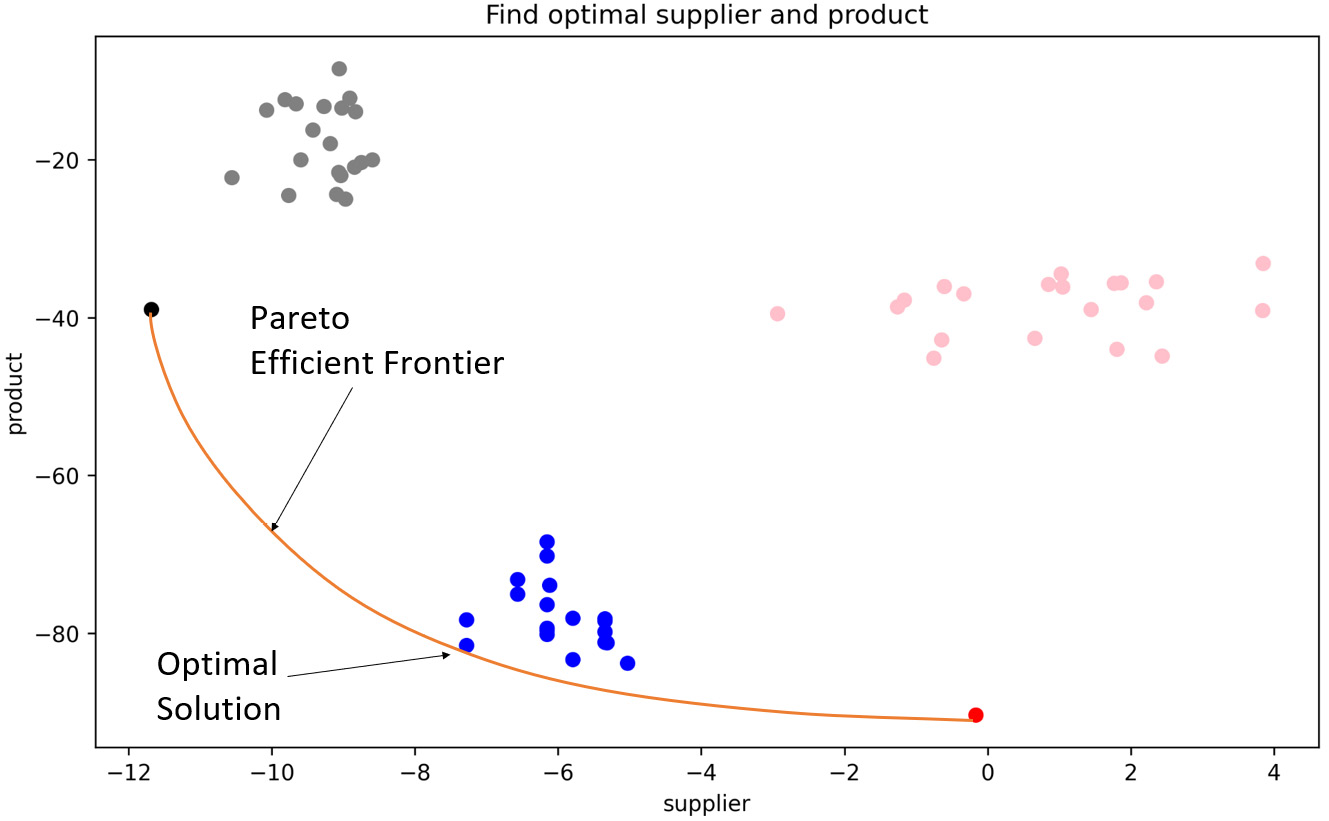
Figure 12.14 – Optimal solution found by selecting the highest energy global score from feasible solutions

The ideal solution is to find a compromise for both the inventory and procurement managers. However, they cannot do better than this if they are to take the global benefit of the store into account. The managers and store leadership can now align their objectives and compensation the structure toward a global strategy. This strategy, if implemented as a global objective, will result in managers cooperating and streamlining operations, as shown in the following diagram:

Figure 12.15 – Global optimization of multiple objectives resulting in better performance

We have now concluded the multi-objective optimization exercise using D-Wave through Amazon Braket. Due to a large number of variables in this example, it was not possible to run this model on the currently available gate-based quantum devices. However, as soon as new devices that can handle 110 or more variables are added to Amazon Braket, the same Mf matrix that we sent to the D-Wave annealer can be sent to the quantum_device_sampler() function to get solutions from gate-based quantum computers.

Summary

In this chapter, we extended our use of Amazon Braket devices to a mock multi-objective optimization problem. We showed the process it would take to map real-world problems to quantum devices on Amazon Braket. Without a rigorous mathematical derivation, we were able to leverage D-Wave to provide an optimal global solution. This type of technique may become important as system and business analysts start using Amazon Braket to solve optimization problems, as well as start re-analyzing their business processes in terms of quadratic relationships and global objectives that may not have been considered or ignored in the past due to classical solver limitations.

Further reading

To learn more about the topics that were covered in this chapter, take a look at the following resources:

• For a rigorous list of mathematical derivations of QUBOs, including set cover, please check out the following links:
  • https://www.researchgate.net/publication/235702677_Ising_formulations_of_many_NP_problems
  • https://arxiv.org/abs/1811.11538
• The following CDL hackathon code might be helpful if you wish to do a more rigorous mathematical evaluation with a problem similar to the one that was presented in this chapter: https://github.com/CDL-Quantum/Hackathon2021/tree/main/ZebraKet.
• The techniques you’ve learned about in this chapter can be used to solve slightly more complex problems, including portfolio optimization, which is also a multi-objective problem with constraints on the number of assets and the need to find feasible solutions. You are encouraged to read the following papers:
  • https://www.researchgate.net/publication/342706781_Portfolio_Optimization_of_40_Stocks_Using_the_DWave_Quantum_Annealer
  • https://www.researchgate.net/publication/343786420_Portfolio_Optimization_of_60_Stocks_Using_Classical_and_Quantum_Algorithms
• The knapsack formulation was used to solve a COVID optimization problem. First, we developed the disease evolution model (SEIRD) and then optimized it to find if a region should be locked down or kept open based on the amount of hospital capacity. The starter code for a basic (SIR) model can be found here, along with the final paper:
  • https://github.com/AlignedIT/SIR-Model
  • https://www.medrxiv.org/content/10.1101/2021.06.14.21258907v1.full
• More samples and further learning opportunities can be found by reviewing the following Amazon Braket and D-Wave examples:
  • https://github.com/aws/amazon-braket-examples
  • https://github.com/dwave-examples
• Please reference the Amazon Braket documentation for any code changes: https://docs.aws.amazon.com/braket/latest/developerguide/what-is-braket.html.

Code Deep Dive

Please review the code in the following functions, which have been used previously in this book:

• run_dwave()
• ProbabilisticSampler()

Please review the code in the following new functions, which were introduced in this chapter and were provided as part of the discussion. They can be found in the code for this chapter in this book’s GitHub repository:

• item_m()
• availability()
• SetCoverSampler()

The following are links to some commonly used quantum computing libraries and platforms:

• https://quantum-computing.ibm.com/
• https://qiskit.org/textbook/preface.html
• https://docs.rigetti.com/qcs/
• https://grove-docs.readthedocs.io/en/latest/index.html
• https://xanadu.ai/
• https://pennylane.readthedocs.io/en/stable/
• https://www.dwavesys.com/
• https://cqcl.github.io/tket/pytket/api/index.html
• https://quantumai.google/
• https://ionq.com/
• https://developer.nvidia.com/cuquantum-sdk
• https://cqcl.github.io/lambeq/index.html
• https://quantumai.google/openfermion
• https://qiskit.org/documentation/nature/

The following are books I highly recommend to dive deeper into quantum computing:

• https://www.amazon.com/Quantum-Programming-Illustrated-Aleksandar-Radovanovic-ebook/dp/B08B3MVXHB
• https://www.amazon.com/Essential-Mathematics-Quantum-Computing-complexities/dp/1801073147
• https://www.amazon.com/Dancing-Qubits-quantum-computing-change/dp/1838827366
• https://www.amazon.com/Quantum-Chemistry-Computing-Curious-Illustrated/dp/1803243902
• https://www.amazon.com/Quantum-Computing_-An-Applied-Approach/dp/3030832732

Concluding section 3

This section was intended to show you a few examples of how real-world problems can be mapped to quantum computers and D-Wave’s quantum annealer. We leveraged Amazon Braket Jobs, which allows users to run many quantum tasks within one job. We also showed how a QUBO is required to rigorously map a real-world optimization problem to a quantum computer or quantum annealer. Then, we saw how a multi-objective optimization problem can be quickly set up without rigorous mathematics.

With this, we have concluded this chapter and also this book. Some examples are included in the Further reading sections at the end of every chapter, and I would consider these good next steps to investigate. It would also be a good idea to dig into the code and functions that we have covered at a high level in this book. This will make it easy for you to make adjustments as new devices are added and new features become available in Amazon Braket. More importantly, I hope that you will create unique libraries for how you utilize Amazon Braket and add more use cases.

Even though this book focused mostly on optimization, many other use cases can be explored, including other basic quantum algorithms, simulation problems, natural language processing, and quantum machine learning. This was intended to be a starting point and to quickly get you comfortable with some basic concepts that lead to useful applications of quantum computing. Ongoing research and improvements are being to all quantum algorithms and you can try refining them. In most cases, please keep in mind that there is considerable mathematics and quantum mechanics rigor, research, and theory behind all the ideas I presented in a simplified manner in this book.

Finally, Amazon Braket was never intended to be an isolated platform. I structured this book so that you can write code and functions while using minimal additional libraries. This gives you the option to add the full capacity of other quantum computing libraries and other AWS services. I have added a few commonly used quantum computing platforms to the Further reading section.

I hope that the experiments in this book have helped accelerate your understanding of quantum computing. I wish you all the best on your continued growth and journey in this exciting area!