
7
Using Gate Quantum Computers – Basic Quantum Algorithms
In this chapter, we’ll continue exploring gate quantum computers and dive further into building some basic algorithms using gates. In the previous chapter, we introduced various gate operations and showed how quantum gates were randomly used to compare a quantum circuit with classical results in the Google supremacy experiment. However, in this chapter, we will use gates in a more meaningful way to show that certain, specific calculations can be performed on quantum computers that are dramatically different from the way calculations are performed on a classical computer. Several very famous algorithms have been developed for quantum computers over time. In this book, we will focus on only a few of these algorithms by experimenting with Amazon Braket simulators and external devices. Our goal is to develop a general intuition of how information is stored on qubits and how it can be manipulated. For examples of other quantum algorithms, as well as a deep dive into the algorithms covered here, please review the Further reading section.
In Chapter 6, Using Gate-Based Quantum Computers – Qubits and Quantum Circuits, we introduced the Bloch sphere and showed how the qubit vector was defined by its angle from the vertical z-axis, as well as its angle around the equator, which is measured from the |+⟩ state. The former can be used to calculate probability amplitudes and thus the probability of measuring qubit states, while the latter represents a phase angle. We also covered how a Hadamard gate or operator moves the qubit vector from the |0⟩ state, which is on the z-axis, to the |+⟩ state at the equator, after which we can rotate the vector along the equator using various gates that produce a z rotation and introduce phase information. This chapter will deal with information along the z-axis, also known as the Computational basis, and phase information, which we will refer to as the Fourier basis.
The ability to increase the probability of measuring a state is known as amplitude amplification. It is a key component of Grover’s algorithm, which is used to bring out the values we are searching for that are stored in a circuit. This is called an Oracle.
We will also learn how to move information between the Computational basis and the Fourier basis using a quantum algorithm called the Quantum Fourier Transform (QFT). The QFT and its inverse are used frequently in quantum computing and are key components of Shor’s algorithm, which leverages QFT. We will also see how QFT is used in addition, by adding to the phase information of a set of qubits.
In this chapter, we will cover the following topics:
- What is a quantum Oracle?
- Observing the effect of amplitude amplification
- Working with phases
Technical requirements
The source code for this chapter can be found in this book’s GitHub repository at https://github.com/PacktPublishing/Quantum-Computing-Experimentation-with-Amazon-Braket/tree/main/Chapter07.
What is a quantum Oracle?
In a classical computer, information is stored in memory or a database. Typically, when we perform operations, the data is copied from its storage location to the CPU so that the operation can be performed. If we are searching for a value in a string, an array, or a database, this operation must read the memory and decide whether we have found a match or not. All this happens very fast and under layers of software that instruct the computer to perform the action in the most efficient manner at the processor level.
If we are going to search for a number in a database, or if we are going to determine which bits in memory are a 0 versus a 1, then at the lowest system level, the data must be read in groups of bits from memory and compared. At the time of writing, there is no equivalent to random-access memory (RAM) or read-only memory (ROM), nor a database that can store information for a long time so that it can be accessed as needed. The simple circuits we created in the previous chapters started with a quantum register with all the qubits initialized to a |0⟩ state. Then, we added gates to implement the operations. If we wanted the qubit to start in a |1⟩ state, we would use an X gate and switch the value of the qubit to a |1⟩ state. This, in effect, is a way to bring data into a quantum register. What if we wanted to simulate a function that returns a specific value, or a conditional clause that returns specific values based on the input states? Since we can’t fully implement RAM, ROM, a database, or a function, we must add it to the circuit as a sort of black box with the answer already programmed. This is called the Oracle. Then, we operate on the Oracle, assuming that, in the future, it will represent a futuristic quantum memory of sorts, where all the values are stored in a long-term superposition. Then, based on the algorithm, we can perform our operation and reveal the answer.
It may almost seem like cheating if we add an array while knowing where the hidden value is, only to then search for it; or convert a number into phase information, only to use an algorithm to reveal it from the phase information. We should also note that this process requires loading all the data or information in advance of running our algorithm. To some extent, the very act of loading the information means that you know all the information. However, that is the situation currently. In code, I can just use the db variable to store the initial value or circuit – this will be our Oracle. Hopefully, in the future, we will have a quantum database that we can point to and perform our operations on, but for now, this Oracle or database will need to be set up in the circuit initially.
We will use this Oracle in our first algorithm.
Observing the effect of amplitude amplification
We have already learned that, in a quantum system, we can have 2n states, where n is the number of qubits. One of the advantages of a quantum computer is that you can control those variables. For example, let’s say that we want to embed a number, such as 2, in a quantum computer so that when we measure the quantum system, the variable 2 (or 10 in binary) shows up with the highest probability possible. How could we selectively add these desired numbers to a quantum circuit?
Let’s work through this example, which is a slightly different way to approach amplitude amplification, though I hope it will make the whole process clearer.
Our goal is to measure the desired numbers in the output with high probability; the remaining numbers should have a low probability. One way to do this would be by creating a matrix that stores our numbers and then running an operator that will amplify the amplitude of those numbers.
We will represent the position of the value(s) we want to embed along the diagonal, as follows:

The value that we want to store will become a -1, while the rest of the diagonal elements will be 1s. The non-diagonal values will remain as zeros. So, if we want to embed the number 2 (or 10 in binary), then the matrix must look like this:

If we create a circuit that represents this and then measure the qubits, we won’t see 10 as the predominant probability, so we need a circuit that can bring the number out or find it if it is stored in the Oracle. Some of the quantum circuits that represent these matrices are more difficult to create than others, and this is an active area of research. A simple circuit to create the number 3 can be created using a new two-qubit gate called the CZ gate. The matrix representation of the number 3 (or 11 in binary), also known as the CZ gate, is shown here:

We will store this number in the Oracle so that it will be represented as the db database in terms of code.
The operator that will be applied to this matrix is called the Grover operator and it will increase the amplitude or probability of finding the |11⟩ state. In this experiment, we won’t worry about the actual process in which amplitude amplification works. Fortunately, it has been covered in many books, so some references to them have been provided at the end of this chapter in the Further reading section.
You have been provided with three functions:
- init_db(n): This function allows you to initialize the quantum register using n as the number of qubits. This also limits the range of numbers you can store from 0 to 2n. The return values include the db database and the maximum value, which is 2n.
- insert_db(values, db): This function will allow you to save a range of values in the Oracle or db. Note that values is a list, so if we want to store 0 and 3, we must pass [0,3].
- query_db(db, n, m, limit=0, local=True, device_name=""): This will apply the Grover operator to the Oracle and increase the amplitude of the value(s) we have stored.
Grover's operator using unitary matrices
In this section, we will show the validity of this concept using only unitary matrices for both the database and Grover’s operator. This allows us to have complete flexibility over the values that have been embedded and use as many qubits as allowed by the simulator.
Let’s try out the Grover operator in terms of code:
- First, we will create and initialize a circuit of two qubits using init_db() and print out the matrix:
Qubits=2
db, dim=init_db(Qubits)
print(db)
Output:
range= 0 to  3
[[1. 0. 0. 0.]
 [0. 1. 0. 0.]
 [0. 0. 1. 0.]
 [0. 0. 0. 1.]]
This is just an initialized matrix and contains 1s in the diagonal.
- Now, let’s insert 3 using insert_db, as shown here:
db, m = insert_db([3],db)
print(db)
Output:
3 added to db
[[ 1.  0.  0.  0.]
 [ 0.  1.  0.  0.]
 [ 0.  0.  1.  0.]
 [ 0.  0.  0. -1.]]
The last diagonal has a -1 in it now. We are ready to send this to the Grover operator.
- The query_db function will apply the Grover operator, measure the qubits on the local simulator, and provide the results:
result=query_db(db, Qubits, m ,1)
Output:
total size 4
qubits 2
db reads 1
{3: 1000}
The following bar chart shows that only the number 3 has been measured:

Figure 7.1 – Measuring the value of 3 after storing it in the database and using the Grover operator
- Now, let’s repeat this process and store 0, 15, 16, 41, 140, 200, 255 in an 8-qubit register. We must start with the following code:
Qubits=8
db, dim=init_db(Qubits)
db, m = insert_db([0, 15, 16, 41, 140, 200, 255], db)
print('total hidden values',m)
Output:
range= 0 to  255
0 added to db
15 added to db
16 added to db
41 added to db
140 added to db
200 added to db
255 added to db
total hidden values 7
- Now, let’s query the database and reveal the values that have been measured in the bar chart:
result=query_db(db, Qubits, m ,1)
The following chart shows the numbers that we had initially embedded in the database showing up with high counts:

Figure 7.2 – Embedded values revealed after applying the Grover operator and measuring them
- Now, let’s send a 7-qubit database to an Amazon Braket simulator. As you may recall from the previous chapter, TN1 cannot process a unitary matrix, while SV1 can process up to a 7-qubit matrix as a unitary. Therefore, let's embed the same numbers in a 7-qubit system and then send it to SV1:
Qubits=7
db, dim=init_db(Qubits)
db, m = insert_db([0, 15, 16, 41, 140, 200, 255], db)
print('total hidden values',m)
Output:
range= 0 to  127
0 added to db
15 added to db
16 added to db
41 added to db
140 is too large, ignored
200 is too large, ignored
255 is too large, ignored
total hidden values 4
Notice that some of the values were not stored because our database is not large enough.
In the next line, we will get the results.
- Let’s query the database by passing it to the SV1 simulator using the following code:
result=query_db(db, Qubits, m, 0, False, 'SV1' )
The following chart shows the results of the values that were saved in the database:
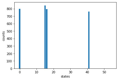
Figure 7.3 – Result of using the Grover operator on SV1
So far, we have tried embedding different values in a database represented by a matrix and showed that, using a unitary simulator, the Grover operator can ensure that the stored numbers are converted into higher probability amplitudes for those states. In the next section, we will do the same process on a gate quantum device.
Grover's search algorithm using quantum circuits
Now, let’s attempt to do the same process that we followed in the previous section, only now using quantum gates and a quantum circuit that represent both the number that is being embedded and the Grover operation. We can also run this on a gate quantum computer. Since we are not using a matrix, there are limitations in terms of building the Grover operator as the key component is a multiple control Z gate. For our purposes, the CCX, which is a 3-qubit gate, and the CCCX, which is a 4-qubit gate, have been defined within the query_circuit_db() function. This will allow us to use the Grover operator with a database using up to 4 qubits. We can demonstrate this using a simple circuit and embed six numbers in the 4-qubit database.
Let’s start with the simple example of embedding 3 in a 2-qubit database:
- 3 has already been embedded in a 2-qubit database using the CZ gate. This gate can be seen in Figure 7.3. As shown there, the last diagonal value is -1. The first part of the circuit is shown here:
db=Circuit().cz(0,1)
print(db)
Output:
T  : |0|
q0 : -C-
      |
q1 : -Z-
T  : |0|
The circuit shows the CZ gate between qubit 0 and qubit 1. This represents how to create the Oracle. Now, let's add the Grover operation.
- Let’s run the circuit using the query_circuit_db() function. Notice that we add the database, the number of qubits, and the number of values stored in the database as parameters:
result=query_circuit_db(db, 2, 1)
Output:
T  : |0|1|2|3|4|5|6|
q0 : -H-C-H-X-C-X-H-
        |     |
q1 : -H-Z-H-X-Z-X-H-
T  : |0|1|2|3|4|5|6|
The following chart shows that we can reveal a value of 3 from the database. This run was made on a local simulator:
Figure 7.4 – A value of 3 has been revealed from the Grover search using a quantum circuit (there is only one bar at 3; please ignore the fractional values on the x-axis)
- Next, we will create a 3-qubit Oracle and store two numbers – that is, 5 and 6. If we visualize the matrix, it will have eight diagonal elements. We want to have the diagonal elements that represent the numbers 5 and 6 have a value of -1. We can do this by using two CZ gates – one between qubit 0 and 1 and the other between qubit 0 and 2. We can do this using the following circuit:
db=Circuit().cz(0,1).cz(0,2)
print(db)
Output:
T  : |0|1|
q0 : -C-C-
      | |
q1 : -Z-|-
        |
q2 : ---Z-
T : |0|1|- Again, let’s use the query_circuit_db() function to reveal the circuit and the values stored in the Oracle. Notice that the circuit that’s been implemented is much longer. The following code is creating the 3-qubit CCZ gate out of the allowed gates:
result=query_circuit_db(db, 3, 2)
Output:
T  : |0|1| 2 |3|4|5|6 |7|8|9|10|11|12|13|14|15|16|
q0 : -H-C-C---H-X------C--------C--C--T--C--X--H--
        | |            |        |  |     |
q1 : -H-Z-|-H-X---C----|---C-T--|--X--Ti-X--X--H--
          |       |    |   |    |
q2 : -H---Z---H-X-X-Ti-X-T-X-Ti-X--T--X--H--------
T : |0|1| 2 |3|4|5|6 |7|8|9|10|11|12|13|14|15|16|- Finally, let’s create a 4-qubit Oracle and store six numbers in it. It turns out that adding two CX gates – one from qubit 0 to qubit 1 and the other from qubit 2 to qubit 3 – creates this effect. This Oracle can be created like so:
db=Circuit().cz(0,1).cz(2,3)
print(db)
Output:
T  : |0|
q0 : -C-
      |
q1 : -Z-
q2 : -C-
      |
q3 : -Z-
T : |0|- To ensure that we have the desired circuit, let’s quickly check it using a matrix representation of the gates and tensor product. In this step and the next, we will take a detour to build the matrix from CZ gates and confirm it has the -1 values in six positions on the diagonal. The matrix representation of the CZ gate is shown here:
#CZ=|0⟩⟨0|⊗I+|1⟩⟨1|⊗Z
arr_cz=np.kron([[1,0],[0,0]],arr_i)+np.kron([[0,0],
               [0,1]], arr_z)
print(arr_cz)
Output:
[[ 1  0  0  0]
 [ 0  1  0  0]
 [ 0  0  1  0]
 [ 0  0  0 -1]]
Let’s perform a tensor product on two CZ gates (CZ ⊗ CZ) to produce the matrix representation:
arr_czcz=np.kron(arr_cz,arr_cz)
print(arr_czcz)
Output:
[[ 1  0  0  0  0  0  0  0  0  0  0  0  0  0  0  0]
 [ 0  1  0  0  0  0  0  0  0  0  0  0  0  0  0  0]
 [ 0  0  1  0  0  0  0  0  0  0  0  0  0  0  0  0]
 [ 0  0  0 -1  0  0  0  0  0  0  0  0  0  0  0  0]
 [ 0  0  0  0  1  0  0  0  0  0  0  0  0  0  0  0]
 [ 0  0  0  0  0  1  0  0  0  0  0  0  0  0  0  0]
 [ 0  0  0  0  0  0  1  0  0  0  0  0  0  0  0  0]
 [ 0  0  0  0  0  0  0 -1  0  0  0  0  0  0  0  0]
 [ 0  0  0  0  0  0  0  0  1  0  0  0  0  0  0  0]
 [ 0  0  0  0  0  0  0  0  0  1  0  0  0  0  0  0]
 [ 0  0  0  0  0  0  0  0  0  0  1  0  0  0  0  0]
 [ 0  0  0  0  0  0  0  0  0  0  0 -1  0  0  0  0]
 [ 0  0  0  0  0  0  0  0  0  0  0  0 -1  0  0  0]
 [ 0  0  0  0  0  0  0  0  0  0  0  0  0 -1  0  0]
 [ 0  0  0  0  0  0  0  0  0  0  0  0  0  0 -1  0]
 [ 0  0  0  0  0  0  0  0  0  0  0  0  0  0  0  1]]
According to the preceding output, we should expect to get 3, 7, 11, 12, 13 , and 14 as the numbers that are stored in the gate circuit's equivalent version.
- Now, let’s run the Grover search on the gate circuit Oracle with two CZ gates:
result=query_circuit_db(db, 4, 6, 3)
You will notice quite a large circuit in the output that also states db reads 3. This means that the Grover operator was run on this circuit three times. Why is this necessary? Before we answer this question, we can confirm that the following chart shows the appropriate values (3, 7, 11, 12, 13, and 14) with the higher counts:
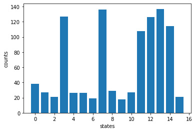
Figure 7.5 – Values detected from using the Grover search on an Oracle with CZ ⊗ CZ
Repetitions of the Grover diffuser operator
In the previous section, we saw db reads 3 in the output. This is the number of times the Grover operator was repeated. The number of times the operator is used can be calculated as follows:
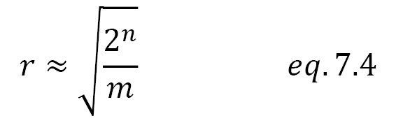
Here, n is the number of qubits, and m is the number of values stored.
In the query_circuit_db() function, the fourth parameter allows you to bypass the default calculation and limit or exceed the ideal value of r. This allows you to visually see the effect of each Grover operator on the amplification of the desired values. You may want to try this out and see what results you get.
Using Grover's algorithm in searches
In the previous subsection, we experimented with a function that implemented Grover’s operator. We showed that if we were to store a set of numbers in an Oracle, then Grover’s operator would only amplify the probability amplitudes of those numbers. In our case, we already knew the number. However, if the Oracle was part of a larger circuit or, in the future, it represented a quantum database search algorithm, the Grover operator would return the required search results. In addition, conditional clauses can also be created using quantum circuits so that they create the same effect in the Oracle.
In this section, we learned how to embed one or more numbers into a qubit and then use the Grover operator to amply the probability of measuring those specific numbers. This technique can be used to search for hidden values in an unstructured list. In the next section, we will look at another way of storing and transforming information in qubits.
Working with phases
In this section, we will discuss how information is stored in qubits in the measurement axis or the z-axis, also called the Computational basis, and the phase angle, which we will refer to as the Fourier basis. It is possible to store information in the phase angle of the qubits and then translate it into the measurement basis. In the next section, we will learn how to think about numbers and their representation in the phase angle of a qubit.
Let’s start with the a variable, which represents a binary number. In our example, we will use a 5-bit number – that is, a=11111. To represent this binary number, we need a register of 5 bits. We can convert this number back into decimal by using the following equation:

This will result in the following equation:

In terms of our example, where we are using a=11111, we will get the following equation:

Here, you can see that a4 has a contribution of 16 to a, while a0 only has a contribution of 1 to a. It is clear that the value of a = 16+8+4+2+1=31.
In other words, our values go from 0, where digits a0 to a4 are 0 to 31, where all digits are 1. If we were to represent this as a circle split into 32 sections, then we could fill the contribution of each digit as follows:

Figure 7.6 – Circle divided into 32 segments to represent 11111
If we only had four right-most bits, then we would have a total of 16 different values. By doing this, we could represent 1111 in the following way, ensuring that we take the contribution of each binary digit:

Figure 7.7 – Circle divided into 16 segments to represent 1111
Going further down the number of bits, if we only had 3 bits, then we could create a circle with eight segments. The contribution of each binary digit would be represented in the circle like so:
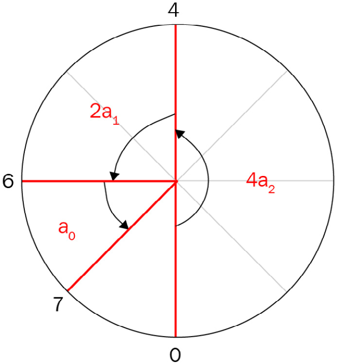
Figure 7.8 – Circle with eight segments to represent 111
We can continue this down to 1 bit. The following diagram shows the contributions of each bit as we move from all 5 bits down to a single bit:

Figure 7.9 – Representation of 11111 on an incrementally smaller number of bits
Now, let’s represent a different number to provide context. We can represent a= 3 using 5 bits, as follows:

Once again, we get the following equation:

Thus, we get the following output:

This can be represented like so:
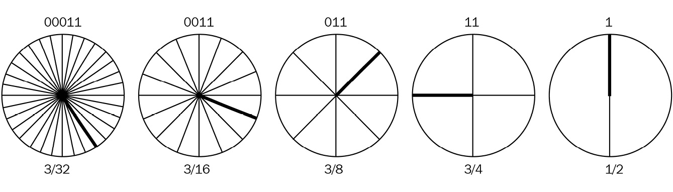
Figure 7.10 – Representation of 3 on incrementally smaller bit circles, starting with 5 bits
Note that on the left-hand side, we are representing the full number, 00011, which is 3 segments out of 32. However, as we reduce the number of bits, we reach a point at 1 bit where we cannot fully represent 3 anymore since it is represented by 11 in binary. The single bit can only hold a value of 1, so we can only represent one out of the two segments.
Repeating the same process for b= 5 with 5 bits, we can use the following equation:

In this case, we get the following equation:

Thus, we get the following output:

We can represent b with the circle segments, as shown here:
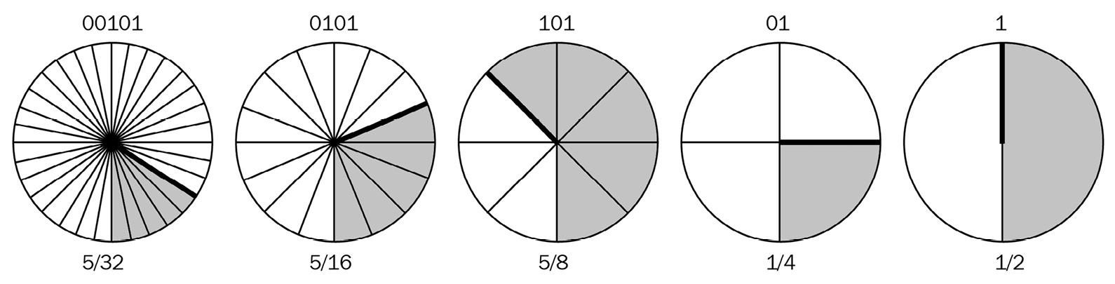
Figure 7.11 – Representation of 5 on incrementally smaller bit circles, starting with 5 bits
Notice that, with the left-most circle, we are moving 5 segments out of 32. The same goes for the 16-segment circle and even the 8-segment circle as the number of bits is reduced. Now, as we reach the 4-segment circle, we are only able to take on the two right-most digits – that is, 01. This is only 1 segment out of the 4. Finally, we end up with the right-most circle, which has the number 1 and thus uses one of the two segments.
We will use the same concept to store a number in the phase of qubits. If you imagine each circle as a view from the top of a Bloch sphere, looking down at the cross-section at the equator, then the rotated line represents how much the vector is rotated in the counterclockwise direction from the bottom, which represents zero degrees.
In the next section, we will review moving the qubit vector between the Computational basis and the phase angle, also known as the Fourier basis.
Note – Drawing Circuits and the Bloch Sphere
We are going to be using the draw_circuit() function, which was introduced and created in the previous chapter. Please refer back to the initial part of that chapter and the relevant GitHub code before proceeding. This function can only be used for one qubit circuit since the Bloch sphere can only represent one qubit.
Translating between the Computational basis and the Fourier basis
We have frequently used the Hadamard gate to move a qubit from the z-axis to the equator of the Bloch sphere. Let’s repeat this process and add a small phase using the T gate. Then, we will use the Hadamard gate again and see what happens:
- First, let’s create a circuit and apply the Hadamard gate and the T gate to a single qubit, as shown here:
circ=Circuit().h(0).t(0)
draw_circuit(circ)
Output:
T  : |0|1|
q0 : -H-T-
T  : |0|1|
Additional result types: StateVector
Matrix:
[[0.70710678+0.j ]
 [0.5       +0.5j]]
State Vector: |psi> = sqrt( [0.5] ) |0> + ( sqrt( [0.5] )) e^i [0.25] pi |1>
The following diagram shows the direction of the qubit vector. The Hadamard gate brings the qubit vector to the |+⟩ state on the equator, and then the T gate rotates the vector along the equator by an angle of π/4 from the |+⟩ state:

Figure 7.12 – Qubit state with a phase angle of π/4 degrees
Output:
T  : |0|1|2|
q0 : -H-T-H-
T  : |0|1|2|
Additional result types: StateVector
Matrix:
[[0.85355339+0.35355339j]
 [0.14644661-0.35355339j]]

State Vector: |psi> = sqrt( [0.85355339] ) |0> + ( sqrt( [0.14644661] )) e^i [-0.5] pi |1>
The following diagram shows the vector moving back up, but not exactly at the |0⟩ state. The phase information is carried over to the measurement basis. Here, we can see that the probability of measuring a 0 has reduced to 0.85, while the probability of measuring a 1 has increased to 0.14:

Figure 7.13 – Bloch sphere showing the resulting qubit state
In this section, we saw that we can treat adding phase information and measurement along the z-axis as a way to convert or translate from one type of information storage into another. In the next section, we will look at more examples of adding phase information to a qubit.
Adding phase information to a qubit
So far, we have learned how a number can be represented as phase angles on a series of circles, as well as how there might be some equivalence between the phase angle and the measurement of the qubit along the z-axis if the information is transferred from one basis to the other. In this section, we will take one qubit and incrementally add a π rotation, then π/2, and then π/4. This is similar to what we did in Figure 7.8. There, with a circle that had been divided into 8 segments, a π rotation represented a value of 4a2, the π/2 rotation represented 2a1, and, finally, the π/4 rotation represented a0. Please refer to that figure to check this.
Now, we will add this same information to a qubit. We will use the phaseshift() function to add the phase to the qubit:
- First, let’s add a π rotation after applying the Hadamard gate to qubit 0:
circ=Circuit().h(0).phaseshift(0,np.pi)
draw_circuit(circ)
Output:
T  : |0|     1     |
q0 : -H-PHASE(3.14)-
T  : |0|     1     |
Additional result types: StateVector
Matrix:
[[ 0.70710678+0.00000000e+00j]
 [-0.70710678+8.65956056e-17j]]

State Vector: |psi> = sqrt( [0.5] ) |0> + ( sqrt( [0.5] )) e^i [1.] pi |1>
The following chart shows that the qubit is pointing to the |-⟩ state with a phase angle of 1.0 pi (this is printed in the last line of the preceding output – that is, e^i [1.] pi):
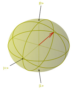
Figure 7.14 – Qubit state at |-⟩ with π rotation
Output:
T  : |0|     1     |     2     |
q0 : -H-PHASE(3.14)-PHASE(1.57)-
T  : |0|     1     |     2     |
Additional result types: StateVector
Matrix:
[[ 7.07106781e-01+0.j        ]
 [-1.29893408e-16-0.70710678j]]

State Vector: |psi> = sqrt( [0.5] ) |0> + ( sqrt( [0.5] )) e^i [-0.5] pi |1>
The following diagram shows the state of the qubit. As you can see, it has rotated counterclockwise by another half of the previous angle. This location is also known as the |-i⟩ state:

Figure 7.15 – Qubit state at |-i⟩ with 3π/4 rotation
- Finally, let’s rotate the qubit further by adding a phase angle of π/4:
circ=circ.phaseshift(0,np.pi/4)
draw_circuit(circ)
Output:
T  : |0|     1     |     2     |     3      |
q0 : -H-PHASE(3.14)-PHASE(1.57)-PHASE(0.785)-
T  : |0|     1     |     2     |     3      |
Additional result types: StateVector
Matrix:
[[0.70710678+0.j ]
 [0.5       -0.5j]]

State Vector: |psi> = sqrt( [0.5] ) |0> + ( sqrt( [0.5] )) e^i [-0.25] pi |1>
We have arrived at the location we wanted with a phase angle of 7π/8 (the same as - π /4), as shown here:
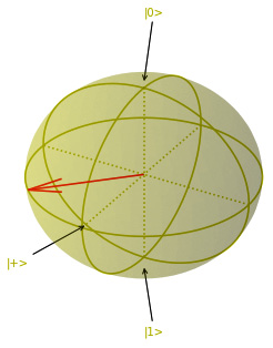
Figure 7.16 – Qubit state with 7π/8 rotation
With that, we’ve learned how to incrementally add phase information in a way that’s similar to adding binary number information to the circles. In the next subsection, we will add a number to the phase information of multiple qubits using the method we have just discussed.
How the phase adder circuit is used in quantum circuits
The phase adder circuit will allow us to add phase information to a set of qubits in the same way as adding a phase to multiple circles. So far, we’ve learned how to move between the measurement x-axis (or the Computational basis) to the Fourier basis, where we can add phase information. Now, we will use the same method to add 3 to the phase angles of 5 qubits. We will add the binary number 00011, as shown in Equation 7.8 to Equation 7.10. In the end, the qubit angles should look similar to those shown in Figure 7.10. The function to set up the desired quantity of qubits and embed the phase rotation based on the number (in decimal) is draw_multi_qubit_phase().
Let’s add the phase information, review how that information would be represented if we were to measure the qubits, and then perform the phase estimation function to convert the phase information into amplitudes that can be measured to reveal the number:
- When we execute the draw_multi_qubit_phase() function, we will get a series of Bloch spheres. The first represents the qubit or bit, 0, associated with a0; the next is qubit 1 associated with a1; and so on. Remember that qubit 0 has two segments, qubit 1 has four, and that qubit 4 has 32 segments:
Qubits=5
Number=3
qc=draw_multi_qubit_phase(Qubits,Number)
Output:
Qubits: 5 Number: 3 binary: 00011
The output also draws the five qubits one after another as can be seen in the GitHub code. The five Bloch spheres have been copied in the figure below to summarize the results.
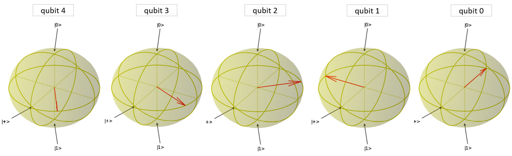
Figure 7.17 – Qubits representing the number 3 in the Fourier basis through phase angles
Output:
T  : |0|     1      |     2      |
q0 : -H-PHASE(3.14)---------------
q1 : -H-PHASE(3.14)--PHASE(1.57)--
q2 : -H-PHASE(1.57)--PHASE(0.785)-
q3 : -H-PHASE(0.785)-PHASE(0.393)-
q4 : -H-PHASE(0.393)-PHASE(0.196)-
T  : |0|     1      |     2      |
Please note that the preceding code just adds the appropriate angles to the qubits. Each qubit is separate and not entangled.
- All the information is in the phase angles. If we were to measure this circuit, which has 5 qubits and therefore 32 possible values from 00000 to 11111, we would have an equal probability of getting each value. We can try this out by running the following code:
device = LocalSimulator()
result = device.run(qc, shots=10000).result()
counts = result.measurement_counts
print(counts)
# plot using Counter
plt.bar(counts.keys(), counts.values());
plt.xlabel('value');
plt.ylabel('counts');
The output is as follows. Notice that no specific information is available in the z-axis, nor the Computational basis that we measured in:

Figure 7.18 – Measurement of the qubits with information on the Fourier basis
- Now, let’s apply another function that will convert the information in the qubit phases into the z-axis. This function contains a series of phase gates based on the inverse quantum Fourier transform. We will use this function to transform the information on the Fourier basis into the Computational basis, where it can be measured. The code for the inverse QFT function, qft_inv_gate(), will be provided. This function represents the phase estimation algorithm. Detailed treatment of both QFT and its inverse has been provided in the Further reading section.
More Details on the Quantum Fourier Transform and Quantum Phase Estimation Algorithms
For our purposes, a detailed treatment of QFT or QPE is not necessary. If you are not familiar with QFT and inverse QFT/QPE or would like to understand these algorithms in more detail, please review the resources in the Further reading section.
To proceed, let's make a copy of our circuit and run the function on the copy. This way, we can use the original circuit again when needed:
qc_copy=qc.copy()
phase_circuit=qft_inv_gate(qc_copy,Qubits)
- Now that we have transformed the phase information into the measurement basis, let’s measure it using the following code:
device = LocalSimulator()
result = device.run(phase_circuit,
                    shots=1000).result()
counts = result.measurement_counts
print(counts)
# plot using Counter
plt.bar(counts.keys(), counts.values());
plt.xlabel('value');
plt.ylabel('counts');
Output:
Counter({'00011': 1000})The preceding output shows 3 in binary, which we originally put in the phase information. The following bar chart also shows this value:
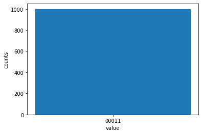
Figure 7.19 – A value of 3 measured after applying the inverse QFT function
With that, we’ve learned how phase information can be converted into measurement information using a function called the inverse QFT. This is a very useful function in many quantum algorithms, including Shor’s algorithm.
In the next section, we will compare the circuit and add phase information with QFT.
Using Quantum Fourier Transform and its inverse
Now that we have learned how to code a binary number into phase information, you will find that the standard way of converting binary information in a quantum circuit into phase information follows the same process. Let’s run the two functions and compare their circuits:
- First, let’s run the function that adds the phase information for the number 3 on only 3 qubits and prints the circuit:
Qubits=3
Number=3
qc=draw_multi_qubit_phase(Qubits,Number)
print(qc)
Output:
T  : |0|     1     |     2      |
q0 : -H-PHASE(3.14)--------------
q1 : -H-PHASE(3.14)-PHASE(1.57)—
q2 : -H-PHASE(1.57)-PHASE(0.785)-
T  : |0|     1     |     2      |
- Now, let’s run the function that will add the number in the circuit using X gates. In other words, it will move the default |0⟩ state to a |1⟩ state, where we have a 1 in the number. Thus, to create 011, we will apply an X gate to the first two qubits. Then, this function will perform a quantum Fourier transform on the qubits to transform the information into the Fourier basis:
device = LocalSimulator()
Qubits=3
num=3
qc=qc_num(num,Qubits)
qc=qft_gate(qc,Qubits)
print(qc)
Output:
T  : |0|     1     |      2       |     3     |4|
q0 : -X-------------C--------------C-----------H-
                    |              |
q1 : -X-C-----------|------------H-PHASE(1.57)---
        |           |
q2 : -H-PHASE(1.57)-PHASE(0.785)-----------------
T  : |0|     1     |      2       |     3     |4|
Here, you can see that the X gate is in qubit 0 and qubit 1, which changes the initial state from |000⟩ to |011⟩. Next, the QFT circuit adds Hadamard gates to the qubit so that phase information will be added. Then, it uses several controlled phase gates to apply the appropriate phase rotations to the required qubit, just like when we applied phase rotations to store the number 3 earlier. One thing to note is that since the circuit only needs to add a Hadamard gate to move a qubit from the |1⟩ state to the |-⟩ state, a π rotation automatically occurs and that rotation does not need to be added to the QFT circuit in qubit 0 and qubit 1, as shown in the circuit in step 1. The rest of the phase angles are the same and the circuits are equivalent. Now, we have two ways to transform a number into a Fourier basis.
- Now, if we do the inverse of the QFT, we should be able to move the phase information to the Computational basis and recover the same number from both circuits:
qc=qft_inv_gate(qc,Qubits)
print(qc)
device = LocalSimulator()
result = device.run(qc, shots=10000).result()
counts = result.measurement_counts
print(counts)
plt.bar(counts.keys(), counts.values());
plt.xlabel('value');
plt.ylabel('counts');
Output:
Counter({'011': 10000})The preceding output shows the number 3 or 011 in binary, as we expected.
Here, we learned that we can convert a binary number into the phase information of qubits programmatically by adding incremental phase rotations, or that we can add the number to a quantum circuit and apply QFT. We also saw that a number in the Fourier basis does not show up when measured. We must use the inverse QFT circuit to move the information to the Computational basis; then, we can measure it.
In the final section, you will learn how to add numbers by adding the phases, thus giving us a circuit that is a phase adder.
Adding numbers using the phase adder
In this section, we will apply the tools we have gained from this chapter to add a number in the phase information of qubits:
- First, let’s create a circuit with the number 3 embedded in the phase of 5 qubits:
Qubits=5
Number=3
qc_3=draw_multi_qubit_phase(Qubits,Number)
print(qc_3)
Output:
Qubits: 5 Number: 3 binary: 00011
- Next, let’s create a circuit with the number 5 embedded in the phase of 5 qubits:
Qubits=5
Number=5
qc_5=draw_multi_qubit_phase(Qubits,Number,False)
print(qc_5)
Output:
Qubits: 5 Number: 5 binary: 00101
Please note that in this case, the function's third parameter is set to False. This will prevent Hadamard gates from being added to the circuit again.
- Now, let’s use the add method from Amazon Braket to add the two circuits together:
qc_total=qc_3.add(qc_5)
print(qc_total)
Output:
T  : |0|     1      |     2      |     3      |     4      |
q0 : -H-PHASE(3.14)—PHASE(3.14)----------------------------
q1 : -H-PHASE(3.14)—PHASE(1.57)—PHASE(1.57)---------------
q2 : -H-PHASE(1.57)—PHASE(0.785)-PHASE(3.14)—PHASE(0.785)-
q3 : -H-PHASE(0.785)-PHASE(0.393)-PHASE(1.57)—PHASE(0.393)-
q4 : -H-PHASE(0.393)-PHASE(0.196)-PHASE(0.785)-PHASE(0.196)-
T  : |0|     1      |     2      |     3      |     4      |
Here, the two sets of instructions, which are mainly phase rotations of the two numbers, have been added to the 5 qubits.
- Now, we just need to perform the inverse of QFT to reveal the added-up phase information:
phase_circuit=qft_inv_gate(qc_total,5)
device = LocalSimulator()
result = device.run(phase_circuit,
                    shots=1000).result()
counts = result.measurement_counts
print(counts)
# plot using Counter
plt.bar(counts.keys(), counts.values());
plt.xlabel('value');
plt.ylabel('counts');
Output:
Counter({'01000': 1000})As you can see, we can recover the number 8 or 01000 in binary.
With that, we have finished experimenting with quantum phase information. We have shown how phase information is stored in qubits and how it can be created using the QFT function. We also reviewed how this information can be added to the Fourier basis and that it can be measured after running the inverse QFT circuit.
Summary
In this chapter, we experimented with some important concepts in terms of quantum algorithms. We used functions to observe how two famous quantum algorithms work. First, we learned about the concept of an Oracle, which stores information that can then be acted upon by the algorithm we are testing. Next, we learned about Grover’s algorithm and how it uses amplitude amplification to increase the probability amplitudes of specific states that represent a hidden number or condition. We saw that this is used by Grover’s algorithm to search for numbers in the Oracle. Next, we understood quantum phase information. We started by looking at examples of incrementally adding rotations that represent the equivalent number of slices in a series of circles. Then, we reviewed the concept of moving between the Fourier and Computational bases and adding phase information to qubits. We prepared qubits with phase information similar to the way we added rotations to the circles to represent a number. This phase information did not produce any information when measured. We had to use the inverse QFT circuit to move the information to the Computational basis before it could be measured. It was revealed that adding phase information to the individual qubits followed a process that was similar to the one that’s used in the QFT circuit and that the two are equivalent. Then, we learned that numbers can be added in the phase of qubits to reveal the sum at the end once the inverse QFT has been applied.
In the next chapter, we will extend our knowledge of quantum algorithms to useful hybrid algorithms. These are algorithms that use quantum computers and require considerable classical computation. We will make use of the QFT, Quantum Phase Estimation, and Phase adder circuits to show how Shor’s algorithm works. In addition, we will investigate more complicated methods to make optimizations using a gate quantum computer.
Further reading
To learn more about the topics that were covered in this chapter, take a look at the following resources:
- Amazon Braket advanced examples showing both QFT and Quantum Phase Estimation (QPE) circuits:
https://github.com/aws/amazon-braket-examples/tree/main/examples/advanced_circuits_algorithms
- A detailed explanation of quantum circuits:
Dancing with Qubits by Robert S. Sutor: https://www.packtpub.com/product/data/9781838827366
Code deep dive:
Several functions were pre-built and provided in this and the previous chapter. You can find these in the GitHub repository for this chapter. Try reviewing the code to see if it is clear based on the steps described in this chapter. Some of these functions are as follows:
run_circuit()
draw_bloch()
draw_circuit()
qc_num()
draw_multi_qubit_phase()
draw_multi_qubit_phase_qc()
qft_gate()
qft_inv_gate()