
5
Using a Quantum Annealer – Developing a QUBO Function and Applying Constraints
In this chapter, we will switch gears from learning about the Amazon Braket service to diving into the programming and basic information needed to solve a real-world problem on a quantum annealer or, more specifically, one of the D-Wave devices available on Amazon Braket.
We will review the concept of quantum annealing, followed by solving a small three-variable problem using D-Wave. Next, we will extend the number of variables and introduce a very simple way to visualize quadratic problems through a party optimization problem. After this, we will use a team selection example to introduce some critical tools, including how to visualize an energy landscape and how to constrain the number of items selected in a solution.
The key sections are as follows:
- Solving optimization problems
- Simulated annealing versus quantum annealing
- Basics of Quadratic Unconstrained Binary optimization (QUBO)
- A QUBO example using three variables
- A party optimization example
- A team selection example
Technical requirement
You can find the code for this chapter under the following GitHub repository:
Since D-Wave now has to be accessed outside of Amazon Braket, refreshed code is provided alongside the original code.
Solving optimization problems
Those familiar with solving machine learning or optimization problems will know that there are algorithms that are frequently used to find the global optimum (minimum or maximum) value of a function. The function is typically called the objective function and has many variables and produces a multidimensional landscape, such as a mountain range, with high and low elevations.
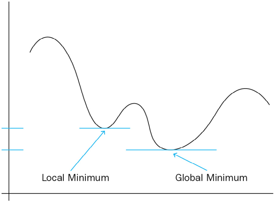
Figure 5.1 – Local minimum versus global minimum
Typical methods used to find the global optimum include gradient descent, simulated annealing, or various genetic algorithms. Even though these are successful and fast algorithms, there is a chance that while searching a large landscape produced by a function with many variables, these algorithms often settle on a minimum (or maximum) that is not the global optimum value but a local optimum. These algorithms use random starting points and probabilistic behavior in moving around a landscape, with the intention of sampling many sections of the landscape to move toward the optimum.
Simulated annealing
Simulated annealing uses a unique technique conceptually based on the real process of annealing. Annealing is a process of heating metals, holding the temperature for a set time, applying additives, and then allowing them to cool to create alloys. It was specifically used to create swords. While hot, the metal allows the additives to disperse, giving it the desired properties. These can include increased strength, a sharper edge, or making a sword less brittle and more flexible in some places, and harder in others. Then, the metal is cooled slowly or rapidly (quenched) to fix the additives in place. This is referred to as the annealing cycle.
In the case of a simulated annealing algorithm, the temperature is simulated by the extent of random changes to the variables to allow a higher amount of sampling of the landscape. Every time the variables are changed, the energy value of the objective function is measured (please refer to Figure 5.2). The similarity to annealing is that this temperature (or the extent of random changes) is adjusted from hot to cold on a desired temperature schedule. This allows the algorithm to sample more parts of the landscape early in the annealing cycle and then narrow in on smaller regions as the temperature is cooled. This is helpful if another valley might be deeper at this initial stage. As the algorithm progresses, the temperature or the randomness is reduced so that the sampling then begins to fixate on the valley it has found and moves down to the minimum. The fact that annealing starts with larger jumps in the beginning when hot and then shorter jumps when cool typically allows the algorithm to jump out of local minimums initially, but then it settles into the minimums of the deeper valleys. The lowest energy value of all the samples then becomes the solution.

Figure 5.2 – Simulated annealing versus gradient descent
With the correct temperature schedule and number of samples, the technique can jump at the right time and not get stuck in local minimums. Of course, with a very complicated landscape, with many deceptively deep valleys that do not contain the global minimum or landscapes with flat plateau regions, it is possible to still not achieve the goal.
Quantum annealing
This is where the Japanese researchers Tadashi Kadowaki and Hidetoshi Nishimori, from the Tokyo Institute of Technology, come in. In a milestone paper, Quantum Annealing in Transverse Ising Model, they proposed that a quantum annealing process could be created where the quantum device would use a very interesting property in quantum mechanics called quantum tunneling. This property appears in quantum mechanics when, for example, a particle is trapped in an energy well or cavity. In this case, based on another rule of quantum mechanics called Heisenberg’s uncertainty principle, it is not possible to know both the location and momentum of a particle with a specific amount of precision. For a particle in a progressively tighter cavity, it would be possible to know its location and then eventually, if it cannot move, its momentum. In other words, in a very tight cavity, a particle should have zero velocity and a precisely known position. Quantum mechanics breaks the particle free of its trap and probabilistically appears outside the cavity. This meets Heisenberg’s uncertainty principle, since the position of the particle becomes probabilistically spread out. This allows a quantum particle to jump barriers that, in our classical world, is not possible. It is this very property we need to jump out of or tunnel through energy barriers if another cavity close to it might lead to a lower value. In the case of quantum annealing, as we saw in Chapter 2, Braket Devices Explained, the qubits start in an initialized energy configuration with the system in the ground state. During the annealing process, the problem coefficients are applied to the qubit bias and coupling terms. We will cover this in detail later in the code; however, for now, this basically changes the energy of each state over the annealing time, as shown in the left plot in Figure 5.3. As the energy landscape changes, initial high-thermal energy allows the system to continue to find and settle in the lowest energy location. Quantum tunneling effects play a role in allowing the system to jump past energy barriers to lower energy states through this whole process, as shown by the curved arrows in the right plot. In the right plot, as time progresses, the ground state changes from 000 to 001 and then 101. As the annealing cycle evolves, the gap between the lowest energy value and the next energy value can become quite small, and sometimes even less than the thermal noise of the qubits. This can cause the state to jump from the lowest energy to the higher energy, which we don’t want. If the process is run slow enough and the temperature is reduced, the tunneling effects can continue to keep the system in its lowest energy past this gap. Finally, the qubits are measured and the ground state is determined. As you can see in Figure 5.3, there are many places where a quantum annealer might jump to the next higher level or not tunnel to stay in the ground energy. This is one reason we sample using many shots and get many different solutions. In the ideal case, we find the ground energy as well.

Figure 5.3 – The quantum annealing process, showing the change of the energy levels through the annealing cycle
In a quantum annealer, the magnetic moments are represented by a +1 or -1 state (called the Ising states or spin states). However, we will only use the QUBO model with 0 and 1 in this book. The magnetic fields (or flux) in the qubits interact with each other and utilize the quantum tunneling effect to switch out of the local minimum toward a lower energy state, leading toward the global minimum. This is what gives a quantum annealer its strength.
We will now move to how we can use the properties of a quantum annealer to solve combinatorial optimization problems. These are problems where two variables affect each other. More specifically, we will deal with quadratic optimization problems where pairs of variables have some defined interaction. More clearly, these are problems where there are no more than two variable interactions. We will learn more about this in the next section.
Quadratic Unconstrained Binary Optimization (QUBO) problems
We will now focus on understanding what kind of problems are solved by a quantum annealer and how a problem is mapped onto the annealer. This process is the same for any solver that can solve QUBO problems. These are a special class of problems where you have binary variables and the relationship between them is no more than quadratic. In other words, you can have the product of two variables but not three variables, and you can have the square of the variables but not the cube or higher. In addition, the variables can only have the values of 0 or 1 (binary) or +1 or -1 (spin).
You can see the following equation as a representation of a QUBO problem. When solving this type of problem, we are trying to minimize the cost function shown in equation 5.1.

This equation can be written in many forms; however, I will use this format so that I can distinguish between the linear terms on the left and the quadratic terms on the right. The equation shows that we are trying to minimize the value of the energy (or cost) as we apply the binary value of 0 or 1 to the xi or xj variables, where i and j are in the range 0 to N-1.
Let’s write this out for an example, where N=3. This means we have three variables, x0, x1, and x2. Each variable has a linear coefficient, a0, a1, and a2 respectively. In addition, we have quadratic terms that are the products of two variables (for example, x0x1). For each of these quadratic terms, there will also be a coefficient, which in this case will be a01.

There are now three linear terms and three quadratic terms. To find the minimum of this cost function, we can randomly try either 0 or 1 for various values of x and then evaluate the result. After trying all combinations, we will find the set of values of x that produce the minimum value for the overall equation. We can then report which x value was a 0 and which was a 1. This would be a brute-force way of finding the minimum.
For very large problems, it is not practical to try out every combination of values of x being 0 or 1; therefore, with many variables (where N is large), we can use a randomized method, where we randomly try out different values for all the x values. This would be a Monte Carlo method, which is basically a random sampling method.
D-Wave’s annealer tries to solve this type of equation and finds the minimum value of the cost function through quantum annealing.
A simple conceptual model for D-Wave
Let’s now spend a bit of time discussing how different values of x can be found for this type of cost function using D-Wave or other QUBO solvers.
First, let’s look at the behavior of magnets. In Figure 5.4, you can see that, in the case of magnets, a north pole attracts a south pole and vice versa. If the magnets are close together, the attractive force is strong, and if they are further apart, the attractive force is weak. We will call this the coupling force between the magnets. If you flip the magnet, then they will repel each other and will want to return to a lower energy configuration by trying to flip over. Again, depending on how close the magnets are, the coupling force that wants the magnets to flip can be small or large.
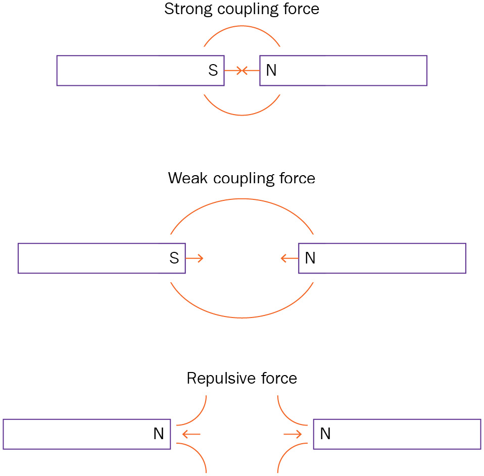
Figure 5.4 – Magnets representing coupling terms
D-Wave uses a quantum property called entanglement with which it can couple the pair-wise behavior between any two given qubits. By entangling all the qubits required in this way, based on the hardware architecture, the problem can be mapped on the annealer. In this case, by changing the coupling strength, we can control the strength by which a pair of qubits will end up with the same value or a different value. We do not need to know the details of quantum entanglement, or how this is accomplished, but for our purposes, it is important to know that a large positive coefficient will force the two pair-wise variables to have the same binary value of 00 or 11, and a large negative coefficient will force the two variables to have an opposite binary value – in this case, 01 or 10. The strength of the value or the absolute value of the coefficient controls how strongly the two values “must” be the same or opposite. Also, if the coefficient is zero, then there is no relationship between the two pairs of variables; thus, they are independent and can both be either 0 or 1 without impacting each other.
A QUBO example using three variables and ExactSolver()
Let’s make this concept more concrete with the example of the three variables. But before we start, we will represent the relationship between each of the values on a grid.

Figure 5.5 – Coefficients showing both linear terms and quadratic interaction terms
We can now see that some values are negative and some are positive. The negative values contribute to a “lower” cost, while the positive values contribute to a “higher” cost. In the grid in Figure 5.5, you can see, for example, the values of a0 = -0.5, a1 = 1.0, and a2 = -0.75. These are the linear coefficients on x0, x1, and x2 respectively. On the other hand, the coupling values, or the influence of one x variable on the other, are also found in the table. The coupling terms are thus a01 = 0.5, a02 = -0.25 and a12 = 0.25. We do not need to fill all the values in the table, as it would be repetitive. The coupling strength between x0 and x1 is the same as that between x1 and x0. There is only one link in the pair-wise coupling.
These relationships can also be represented in the form of a graph with nodes (or vertices) and links (or edges), as shown in the following figure:

Figure 5.6 – Coefficients represented on a graph
These relationships are all we need to find the binary values of x0 to x2, which will minimize the cost function. Let’s write out the full equation with the coefficients now:

Please make sure to compare the coefficients in equation 5.2 with the values in equation 5.3. We can use various methods to solve this and find the values of x0, x1, and x2 that will minimize this cost function, but in our case, we will first use D-Wave’s ExactSolver() function and then, in the next section, we will solve the same problem using D-Wave’s DW2000Q quantum annealer. Let us start by using the ExactSolver() function:
- We will need to import dimod as the only library at this time:
import dimod
- Let’s define the binary quadratic model in dictionary form.
First, we will create the dictionary of linear terms. The a0, a1,and a2 linear coefficients are associated with the x0, x1, and x2 variables:
linear={('x0'):-0.5, ('x1'):1.0, ('x2'):-0.75}
print(linear)
Output:
{'x0': -0.5, 'x1': 1.0, 'x2': -0.75}Next, we insert the quadratic terms using the appropriate coefficients. The a01, a02, and a12 quadratic coefficients are the coupling terms between the pair of x0x1, x0x2, and x1x2 variables.
quadratic={('x0','x1'):0.5, ('x0','x2'):-0.25,
           ('x1','x2'):0.25}
print(quadratic)
Output:
{('x0', 'x1'): 0.5, ('x0', 'x2'): -0.25, ('x1', 'x2'): 0.25}Now, we can use the BinaryQuadraticModel dimod function to combine these two linear and quadratic terms and also identify the variables (x0...x2) as Binary. Remember that we want x0 to x2 to be either 0 or 1:
vartype = dimod.BINARY
bqm = dimod.BinaryQuadraticModel(linear, quadratic,
                                 vartype)
- We are now ready to execute this cost function on the dimod local classical solver function, ExactSolver(), that will accurately produce all the appropriate cost values for the different combinations of x values as 0 or 1. The solution is then sorted with the lowest cost shown first:
sampler = dimod.ExactSolver()
response = sampler.sample(bqm)
print(response)
Output:
  x0 x1 x2 energy num_oc.
6  1  0  1   -1.5       1
7  0  0  1  -0.75       1
1  1  0  0   -0.5       1
0  0  0  0    0.0       1
5  1  1  1   0.25       1
4  0  1  1    0.5       1
2  1  1  0    1.0       1
3  0  1  0    1.0       1
['BINARY', 8 rows, 8 samples, 3 variables]
The first column is a sequence number and can be ignored for this brute-force solver.
The first row of the results shows that the lowest cost solution has a value of -1.5 and requires x0=1, x1=0, and x2=1. The next lowest energy of -0.75 is found when only x2=1, while x0 and x1 are 0.
We have seen how to create a binary quadratic model of a cost function of three variables using a dictionary in Python and then found the minimum of that cost function using the ExactSolver() solver, which is available in D-Wave.
In the next section, we will set up code to find the minimum value of this cost function using the D-Wave quantum annealer.
Running the three-variable problem on D-Wave annealer
In this section, we will set up the D-Wave annealer as a solver and then execute the binary quadratic model on the D-Wave device.
Let’s get started:
- We will import the additional libraries needed to designate D-Wave sampler to perform the embedding:
from dwave.system.samplers import DWaveSampler
from dwave.system.composites import EmbeddingComposite
shots=200
sampler = EmbeddingComposite (DWaveSampler())
Using this method, D-Wave will pick the default device. Later we can learn how to set the appropriate D-Wave device.
- We do not need to set chainstrength with such a small number of variables; the embedding will use one qubit per variable, so there will be no chain of qubits that represent one variable.
Finally, we run the D-Wave sampler using the binary quadratic model of our problem cost function, and the required shots:
#chainstrength = 1
response = sampler.sample(bqm, num_reads=shots)
print(response)
Output:
  x0 x1 x2 energy num_oc. chain_.
0  1  0  1   -1.5     200     0.0
['BINARY', 1 rows, 200 samples, 3 variables]
The solution shows that D-Wave finds x0=1, x1=0, and x2=1 is the best solution, with the lowest cost value of -1.5. Note that D-Wave found this for all 200 shots. This clearly shows that D-Wave was efficiently able to find this lowest energy value from the problem.
We will now recap what we have learned from the results. If we go back to the grid in Figure 5.5, we can see the contributions of the cost from each linear and quadratic term. Each number (or coefficient) supplies a positive or negative cost if it is selected based on the binary variables.
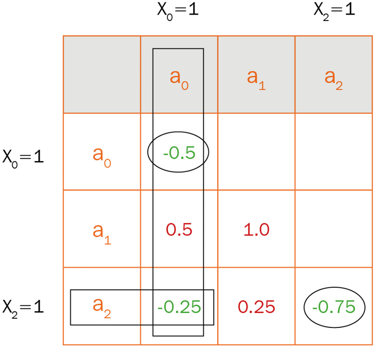
Figure 5.7 – A table showing the contributions of coefficients where xi=1
The way to look at this is that since x0 and x2 have a value of 1 in the solution, then their linear and quadratic coefficients will contribute to the final cost. Based on the table in Figure 5.7, you can see that there are two linear contributions, a0=-0.5 and a2=-0.75 (ovals), which equate to where xi is 1, and one quadratic contribution at a0a2 (where the rectangles overlap), which means we have a single quadratic contribution of -0.25. The sum of these three contributions is -1.75, which is indeed the lowest value we can attain from this problem. Any other combination will add contributions that will have a higher cost value. Thus, the optimal solution is x0=1, x1=0, and, x2=1.
We can also represent the binary values of 0 and 1 as off and on, or in and out. Therefore, we want to set up our problem in such a way that the result tells us something about the condition of the optimal selection. When converting your real-world problem, think of your variables, and determine whether they can be defined as binary. An example could be that you have many hubs that a flight will go to. If the hub is on the flight path, it has a value of 1, and if the flight does not go to the hub, its value is 0.
So far, we have reviewed what quantum annealing is and gone over a very simple example of how to embed an objective function on a quantum annealer using a quadratic binary optimization formulation. We solved a three-variable binary optimization problem on a brute-force solver and then we solved the same problem on a D-Wave quantum annealer device. We have a lot more to learn about embedding real-world problems on D-Wave, visualizing the landscape, and adding constraints. We will now start with a party optimization example.
A party optimization example
In this example, imagine that you are throwing a party and inviting five friends. We will give them unique names from Alice to Frank, as shown in Figure 5.8. You have made an estimate of how much each of your friends contributes to the energy of a party. These are the linear or diagonal terms in the table in Figure 5.8. Your values are from -1 (a negative contribution to the party) to +1 (a maximum positive contribution to the party). For example, Alice has the most positive contribution to a party of 0.5, while Eve who does not contribute to the energy at parties has a value of -1.
Now, you also realize that not only do each of your friends individually contribute to a party’s energy but their energy contribution changes, depending on who else is at the party with them. You are feeling quite sophisticated for having determined that pair-wise relationships or quadratic relationships are important in this case. You recall how each pair of friends contribute to the energy of a party when they are present together. Again, your values are from -1 (negative contribution to the party) to +1 (maximum positive contribution to the party). Thus, Alice and Bob, when together, have the most positive impact at 1.0, while Alice and Eve together have the worst effect on a party at -1.
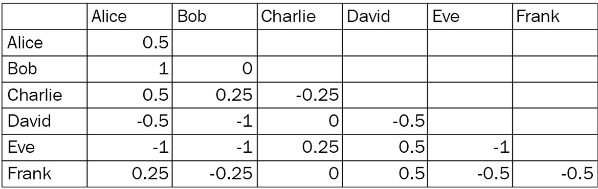
Figure 5.8 – The friends' contribution to a party
Now that you have this information, you want to optimize and find which friends would be the optimal guests at a party with the most energy contribution. You are only going to invite these friends.
Download the party example code from the GitHub site along with the Friends.csv file. Let’s look at the steps needed to solve this problem. Since we only have a few friends, we can run this through ExactSolver():
- First, let’s import the necessary libraries:
import pandas as pd
import dimod
- Then, we load the friends.csv file into a matrix, T. Note that we only have values in the lower-left corner:
file_name='friends.csv'
Temp = pd.read_csv(file_name, ).values
T=Temp[:,1:]
print(T)
Output:
[[0.5 nan nan nan nan nan]
 [1.0 0.0 nan nan nan nan]
 [0.5 0.25 -0.25 nan nan nan]
 [-0.5 -1.0 0.0 -0.5 nan nan]
 [-1.0 -1.0 0.25 0.5 -1.0 nan]
 [0.25 -0.25 0.0 0.5 -0.5 -0.5]]
- Next, we extract the names:
dim=len(T[0])
Names=['']*dim
for i in range(dim):
    Names[i]=Temp[i,0]
print(Names)
Output:
['Alice', 'Bob', 'Charlie', 'David', 'Eve', 'Frank']
- We are now going to create the linear and quadratic terms for the binary quadratic model. Note that we change the sign on the T matrix, since the coefficients represent maximizing the energy, but in our solvers, we always minimize. First, we will view the linear terms:
linear={Names[i]:-T[i][i] for i in range(dim)}
quadratic={(Names[i],Names[j]):-T[i][j] for i in
            range(dim) for j in range(dim) if i>j}
print(linear)
Output:
{'Alice': -0.5, 'Bob': -0.0, 'Charlie': 0.25, 'David': 0.5, 'Eve': 1.0, 'Frank': 0.5}Next, we can also view the quadratic terms:
print(quadratic)
Output:
{('Bob', 'Alice'): -1.0, ('Charlie', 'Alice'): -0.5, ('Charlie', 'Bob'): -0.25, ('David',
'Alice'): 0.5, ('David', 'Bob'): 1.0, ('David', 'Charlie'): -0.0, ('Eve', 'Alice'): 1.0,
('Eve', 'Bob'): 1.0, ('Eve', 'Charlie'): -0.25, ('Eve', 'David'): -0.5, ('Frank', 'Alice'): -0.25,
('Frank', 'Bob'): 0.25, ('Frank', 'Charlie'): -0.0, ('Frank', 'David'): -0.5, ('Frank', 'Eve'): 0.5}- Now that we have our linear and quadratic terms, we will create the binary quadratic model (BQM) and send it to the ExactSolver() function. We only show some of the best results:
vartype = dimod.BINARY
bqm = dimod.BinaryQuadraticModel(linear, quadratic,
                                 vartype)
sampler = dimod.ExactSolver()
response = sampler.sample(bqm)
print(response)
Output:
Alice Bob Charlie David Eve Frank energy num_oc.
5      1   1       1     0   0     0   -2.0       1
2      1   1       0     0   0     0   -1.5       1
58     1   1       1     0   0     1   -1.5       1
61     1   1       0     0   0     1   -1.0       1
6      1   0       1     0   0     0  -0.75       1
1      1   0       0     0   0     0   -0.5       1
57     1   0       1     0   0     1   -0.5       1
62     1   0       0     0   0     1  -0.25       1
The best value is the first row and shows that the best energy for the overall party would be if you invite Alice, Bob and Charlie. The value of the energy is +2.0, after changing the sign.
Can you validate that this is the optimal solution? Was the answer obvious just from looking at the linear and quadratic terms? Can you run the BQM on the D-Wave annealer as we did in the last section and see whether you get the same results?
In the next section, we will look at a more complicated example.
A team selection example
In this example, imagine your manager, the Vice President (VP), just heard about the new capability of quantum computers to solve optimization problems. The VP has been wanting to build a team with key resources in the company based on the following:
- Their individual ratings conducted by the managers
- The ratings given by their peers who worked best together
The values have been averaged over a few years, and the rating given by employee 1 to employee 2 is separate from the ratings given by employee 2 to employee 1 and are usually the same, but in some cases, they are off by 1. The 100 employee names are not disclosed. The ratings go from 0 to 5, with 5 being the highest rating. The VP is looking for a way to incorporate the data to identify 10 key individuals for a special group project where the team score is highest, based on both the manager scores and the pair-wise employee-employee score. The VP also wants you to consider the manager score to have the same weight as each employee-employee pair-wise score; however, they would like to be able to control the ratio. The last statement the VP makes before leaving is, “I want to know the combination of 10 employees that have the highest score as a team and not necessarily those who got the highest total scores individually.”
First of all, let’s look at the last statement. Is there a difference? To understand combinatorial optimization, it is important to grasp the difference between summing up the total individual scores received by the 10 employees, and also adding the pair-wise scores of all the 10 employees selected into the team.
A simple process for solving problems using D-Wave
It is always a good idea to first understand a problem and try to solve it using the current traditional formulation before progressing to converting the problem into a QUBO. This way, you will understand the problem and the assumptions or trade-offs being made when deriving the QUBO. It also gives a good way to benchmark the results. After deriving the QUBO, we solve the problem classically. I have included a tool to visualize the energy landscape, which we will discuss soon. This tool allows you to see where the minimum of the landscape is and what results to expect from a classical QUBO solver, such as a simulated annealer. After we are convinced that we have the correct formulation and the QUBO is producing good results, we can progress to solving it on a quantum annealing device. This also prevents unnecessary waste of money by using a quantum device before we are ready.
After running our first few tests on a quantum device, if we find that the results are not adequate or the energy values are not low enough, we might need to adjust the parameters available to us in the quantum annealing solver (D-Wave 2000Q or D-Wave Advantage).
The preceding steps have been summarized as follows in Figure 5.9. We will follow these steps as we progress through this example.

Figure 5.9 – The steps to solving QUBO problems on D-Wave
Reviewing data
To fully understand the problem as in Step 1 (A) of Figure 5.9, let’s look at the data file and produce a heat map. A heat map of the data is reproduced in Figure 5.10. The diagonal terms are the ratings given by the employee’s manager and seem to generally be higher than the ratings given by one employee for another. Also, note that this is not symmetric. In other words, the values on one side of the blue diagonal do not always match the other side, as can be noted clearly by the red values that are only on the lower-left triangle but not in the upper-right triangle.
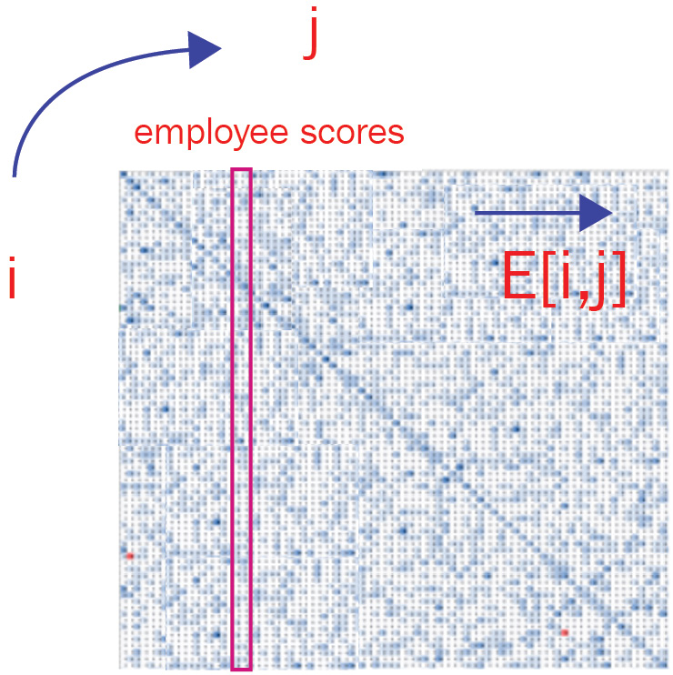
Figure 5.10 – A heat map of the employee score data
The blue arrow indicates that employee i gives a score to employee j. The vertical line represents all the scores given to employee j. The faint blue diagonal line is the score given by the manager to the employee (where i=j). In this example, E[i,j] is not equal to E[j,i], and we will show how this is handled in the next section.
Representing the problem in graph form
We can now represent the problem in the form of a graph and put in some sample values to understand how the scores are represented, as shown in Figure 5.11.
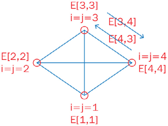
Figure 5.11 – Showing four manager-employee scores on a graph and one pair of employee-employee scores
This is only a partial representation of the whole problem, but it shows some key elements and how they are going to be implemented in code. One thing to note is that since the score given by employee i to employee j is not the same as that given by employee j to employee i, we have a relationship between elements that depends on direction, and this is represented by the two arrows. These two values can be handled by most solvers; however, the D-Wave quantum annealer can only have one relationship between variables or employees in this case, so in order to solve this on D-Wave, we will have to “add” the two E[i,j] and E[j,i] values together and then implement them in D-Wave’s quadratic terms.
Summarizing the problem
Just to get started with the code, we can write down some of the key points from the problem and how we will start formulating them with arrays in Python. These points are jotted down in Figure 5.12.

Figure 5.12 – A summary of the key concepts in the problem
Now, we have completed Step 1 (A) in Figure 5.9 and have a good understanding of the problem.
The traditional formulation
We are ready to start running through the process in the code. We will go to Step 1 (B) in Figure 5.9, where we want to first create the traditional formulation in the code:
- Copy matrix from the file:
import pandas as pd
E = pd.read_csv("employees.csv", header=None ).values
if (len(E[0])==len(E[1])):
 dim=len(E)
 print(dim)
Output:
100
Note that the full matrix is stored in E.
- Now, we want to create the traditional formulation. As was stated in the problem, the VP gives a hint on what the traditional formulation is: "…not necessarily those who got the highest total scores from other employees." Assuming this is the traditional way the VP has evaluated employees, let’s find the employees with the top scores, based on ratings from other employees and the manager. Thus, we just need to add up an employee’s scores, which is equivalent to summing up the column (as shown as the purple vertical rectangle in Figure 5.10.
- After the employee scores are added and sorted, we find the top 10 employees. Please review the code in the chapter’s GitHub repository. The output is as follows:
Employee/score
12 173
92 172
28 169
16 169
65 167
14 167
59 165
23 165
2 165
85 164
We also create a smaller matrix, Top_E, of only the scores of these 10 employees. The team score is calculated as the sum of the smaller matrix of all the manager-employee scores and the employee-employee scores from this subset. The results are sorted by the employee number and the output is as follows:
New Employee Team [ 2 12 14 16 23 28 59 65 85 92]
[[5. 1. 2. 1. 3. 1. 1. 3. 3. 1.]
 [1. 3. 3. 1. 1. 4. 1. 3. 1. 2.]
[2. 3. 3. 2. 1. 1. 3. 1. 1. 2.]
 [1. 1. 2. 3. 2. 2. 1. 1. 2. 5.]
 [3. 1. 1. 2. 3. 1. 2. 1. 1. 1.]
 [1. 4. 1. 2. 1. 3. 2. 1. 3. 1.]
 [1. 1. 3. 1. 2. 2. 3. 1. 2. 2.]
 [3. 3. 1. 1. 1. 1. 1. 3. 2. 1.]
 [3. 1. 1. 2. 1. 3. 2. 2. 3. 1.]
 [1. 2. 2. 5. 1. 1. 2. 1. 1. 4.]]
This team's total score based on this smaller matrix is found to be 189.0. Do you think that this team score is the highest of any other 10-member team? This is the question we are really asking, so let's continue to answer this question.
- It is time to start looking at this problem beyond the traditional way and think about how to convert this into a binary quadratic problem, as stated in Step 2 (A) in Figure 5.9.
In the employee.csv file, the diagonal terms, E[i,i], represent the linear coefficients for the manager-employee score, and the non-diagonal terms, E[i,j], represent the quadratic relationships between pair-wise employees (employee-employee). We can see that it is a binary problem, since we are looking for employees selected into the team or not selected into the team, thus ei = 0 if not selected and ei=1 if selected. Since we want to minimize the energy, we add negative signs to the E matrix. We also know we must add a constraint or penalty so that we only get 10 employees in the answer.


- As shown in Step 2 (B) in Figure 5.9, we need to convert the data to a standard matrix; however, since the data is already presented to us in the form of a matrix, this step is complete.
- In the following code, we send the -Top_E matrix to the simulated annealer:
import neal
import dimod
Nsampler = neal.SimulatedAnnealingSampler()
QDWaveSA = dimod.BinaryQuadraticModel(
  -Top_E, dimod.BINARY)
SAresponse = Nsampler.sample(QDWaveSA)
for Ssample in SAresponse.data():
    print( Ssample)
Output:
Sample(sample={0: 1, 1: 1, 2: 1, 3: 1, 4: 1, 5: 1, 6: 1, 7: 1, 8: 1, 9: 1}, energy=-189.0, num_occurrences=1)We get an energy value of -189. This is the equivalent of the sum we found in Step 3.
- Now, let’s repeat this step for the full matrix, -E:
Nsampler = neal.SimulatedAnnealingSampler()
QDWaveSA = dimod.BinaryQuadraticModel(-E,
                                      dimod.BINARY)
SAresponse = Nsampler.sample(QDWaveSA)
for Ssample in SAresponse.data():
    print( Ssample)
Output:
Sample(sample={0: 1, 1: 1, 2: 1, 3: 1, 4: 1, 5: 1, 6: 1, 7:
1, 8: 1, 9: 1, 10: 1, 11: 1, 12: 1, 13: 1, 14: 1, 15: 1, 16:
1, 17: 1, 18: 1, 19: 1, 20: 1, 21: 1, 22: 1, 23: 1, 24: 1,
25: 1, 26: 1, 27: 1, 28: 1, 29: 1, 30: 1, 31: 1, 32: 1, 33:
1, 34: 1, 35: 1, 36: 1, 37: 1, 38: 1, 39: 1, 40: 1, 41: 1,
42: 1, 43: 1, 44: 1, 45: 1, 46: 1, 47: 1, 48: 1, 49: 1, 50:
1, 51: 1, 52: 1, 53: 1, 54: 1, 55: 1, 56: 1, 57: 1, 58: 1,
59: 1, 60: 1, 61: 1, 62: 1, 63: 1, 64: 1, 65: 1, 66: 1, 67:
1, 68: 1, 69: 1, 70: 1, 71: 1, 72: 1, 73: 1, 74: 1, 75: 1,
76: 1, 77: 1, 78: 1, 79: 1, 80: 1, 81: 1, 82: 1, 83: 1, 84:
1, 85: 1, 86: 1, 87: 1, 88: 1, 89: 1, 90: 1, 91: 1, 92: 1,
93: 1, 94: 1, 95: 1, 96: 1, 97: 1, 98: 1, 99: 1}, energy=
-15304.0, num_occurrences=1)
Here, we get a score of -15,304.0. This represents all the employees. So we really have not found the top 10 employees using this method.
What does this tell us? It is not obvious, but a simulated annealer or any other solver is finding the minimum energy, and since every employee adds to the negative energy in either -Top_E or -E, the best solution is to add up all the employees and give the total energy of the matrix. This would not be the case if there were scores of negative values. For example, if the scores ranged from -5 to +5, then it is possible that the solvers would pick the positive values (in the negative matrix, -E) that would penalize some of the employees and reduce the number of employees in the answer. Somehow, we have to penalize the total matrix so that only 10 employees are picked in the answer. We are coming to this soon, but first, we need to visualize the landscape.
I find it helpful to visualize the landscape using a probabilistic solver. This will show you what your landscape looks like and what answers to expect. We will review this tool in the next section.
A tool to visualize the energy landscape
It is not practical to visualize a multidimensional energy landscape; however, we can organize the energy landscape based on the number of values in the solution. For example, if we have a 100-variable problem, that would mean we are dealing with 100 dimensions, and it would not be practical to visualize the landscape. However, what if we could calculate every solution with one value in it? There are 100 such solutions in a 100-variable problem. We can determine the energy of each of the 1-value solutions and plot those, and then we can look at all the 2-value solutions as combinations out of the total 100 variables. This gives us 4,950 different energy values. This way, we can tell how the energies change based on the number of solutions, or the count, and whether there is a pattern where the energies increase, decrease, or have a minimum somewhere in between.
Figure 5.13 shows an example of different landscapes plotted this way. These plots can easily tell whether the minimum will be where no value is selected (the middle plot in the bottom row), or when almost all values are selected (the right-most plot in the middle row). You can also see that some landscapes are quite complicated, and the minimum can be in a wide range of values. If we do more sampling, we will see the landscape more clearly.
The key point to note is that by using this tool, you can understand whether the landscape will give the expected results. For example, if you have a landscape where the minimum has a large count in the solution and you are expecting to have only a few values in your result, then you might have to add a constraint to change the landscape from the plot shown on the right in the bottom row to the one shown on the right on the top row.

Figure 5.13 – Sample energy landscapes, with the x axis representing the number of values selected in the solution (the count)
When we run the visualization tool, ProbabilisticSampler(), on the -E matrix, we get the plot shown in Figure 5.14. The sample code for this function is included in the GitHub repository of this chapter.

Figure 5.14 – A visualization of the energy landscape
The x axis represents the number of binary variables in the solution that had a +1 value, or the count in the solution. In this case, it is the count of the employees in the solution. The y axis is the energy. You can see that as more employees are selected for the team, the more negative the energy becomes. If this was sent to a quantum annealer, we would just get all the employees in the solution.
It should be easy to realize at this point that sending this to a quantum annealer will not help in any way; it will just give a solution where all the ei variables are equal to 1. We must find a way to bring the minimum of the landscape to where the count or the number of employees selected in the solution equals 10.
ProbabilisticSampler() can be used with the following parameter list:
Parameter list:

Return values:

You can now use this tool to visualize your matrix before sending it to a QUBO solver (a simulated annealer or D-Wave’s quantum annealer). In the next section, we will look at how to convert this landscape to the required count or number of employees in the solution.
A simple penalty function to implement the constraint
Now, we move to Step 2 (C) in Figure 5.9. Let’s look at the penalty term we need for the constraint in equation 5.6. We make it more generic by replacing the number 10 with the M variable and rewriting, as shown here:

This penalty can be converted into the following equation:

This is basically an equation of the y=(x-c)2 form. If you plot this equation for different values of x, you will find it is a parabola with the minimum, where x=c. We use this to add the penalty – that is, employees=10 – to the QUBO. We introduce a multiplier, S, for the strength of this penalty, so it is effective on the rest of the QUBO.
It turns out that expanding equation 5.8 leads to the following equation:

Here, M2 is going to be an offset that we will add to the result of the QUBO. Note that, except for the offset, equation 5.9 is in the same form as our QUBO, with linear and quadratic terms. Thus, we can now add this to our QUBO formulation:


Now that we understand the QUBO and the penalty function, let’s use this information to modify the original matrix, E, to the C matrix by adding the penalty matrix, P. Note that we implement S as the strength variable. To get the correct result, we will pick the value of 90:
- The following code shows how we create the P penalty matrix:
# The constraint matrix
size=dim
max_count=10
strength=90
#strength=1
P=np.ones((size,size))
for i in range(size):
 for j in range(size):
  if i==j:
   P[i,i]=strength*(1-2*max_count)
  else:
   P[i,j]=strength
offset=(max_count)**2
- Now, we need to add Penalty to the original -E matrix:
C=P-E
- We now visualize the landscape by running the ProbabilisticSampler() function again:
min_list, e_min, comb_list=
ProbabilisticSampler(C,1000,offset, 5, 15)
Output:
Best found: [2, 16, 25, 43, 44, 51, 65, 69, 77, 87]
count: 10
Energy: -9103.0
Solutions Sampled: 11000
The plot will show that the minimum is now close to 10, based on the strength of the penalty term used. We also find a valid solution with a count of 10. If it is not, we might need to adjust strength of the penalty.

Figure 5.15 – The modified matrix with the minimum at 10 employees
We can change the minimum and maximum count values to zoom in or out on the energy landscape. This meets our objective for Step 2 (D) in Figure 5.9.
- Since we know where to focus our search, we can increase the sample count and look for more solutions where the count is 10. This takes a while to run:
min_list, e_min, comb_list=
  ProbabilisticSampler(C,100000,offset, 10, 10)
Output:
Best found: [16, 18, 19, 34, 36, 56, 65, 69, 84, 92]
count: 10
Energy: -9126.0
Solutions Sampled: 100000
The plot shows a broad range of values at the single count of 10.
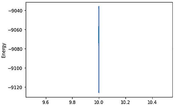
Figure 5.16 – The energy range at the count of 10 with higher sampling
Note that we do not want to use the energy from the plot or a constrained model because it includes the penalty terms and thus does not represent the score. To get that, we need to take the employee numbers in the solution and calculate the score using the original E matrix.
- The following code is used to find the team score of the best solution found in the last step, based on the ratings from others within this team. We use the values from the original E matrix:
Top_e_PS=min_list
# Team score from the original Employee score matrix, using the employee index numbers
team_score=0
for i in (Top_e_PS):
 for j in (Top_e_PS):
 team_score+=E[i,j]
print("Employees", Top_e_PS, "Team Score:",team_score)
Output:
Employees [16, 18, 19, 34, 36, 56, 65, 69, 84, 92] Team Score: 226.0
This score is better than the score found using the traditional method.
Running the problem on classical and quantum solvers
Now that we have sampled the landscape and ensured that the solution is at the correct number of employees, we can proceed with running the modified matrix on the classical simulated annealer and the quantum annealing devices.
Let’s get started:
- We can now run the modified C matrix on the simulated annealer, as stated in Step 3 (A) in Figure 5.9, using the following code:
# Sending All Employee matrix E (using -ve sign for minimization)
Nsampler = neal.SimulatedAnnealingSampler()
QDWaveSA = dimod.BinaryQuadraticModel(C, dimod.BINARY)
SAresponse = Nsampler.sample(QDWaveSA)
for Ssample in SAresponse.data():
    print( Ssample)
Output:
energy=-9178.0
Notice the output is a large negative number because it includes the energy of the penalty. We need to take the resulting values and find the energy for the actual solution.
- Now we determine the energy of the solution:
# print qubits with value 1
best=0
team_score=0
for sample, energy, n_occurences in SAresponse.data():
     sample_list=[]
     for i in range(dim):
         #sample_str.append(str(sample['a'+str(a)]))
         if sample[i]==1:
             sample_list.append(i)
     for i in (sample_list):
         for j in (sample_list):
             team_score+=E[i,j]
     if best==0:
         Top_e_DW=sample_list
         best_DWave_val='best Simulated
           Annealer:'+str(sample_list)+'
           team_score:'+str(team_score)+'
     best=1
     print(sample_list, team_score, len(sample_list),
           n_occurences)
     #break #comment out break to see all values
print(best_DWave_val)
Output:
[0, 1, 4, 19, 23, 45, 47, 59, 78, 95] 194.0 10 1
best Simulated Annealer:[0, 1, 4, 19, 23, 45, 47, 59, 78, 95] team_score:194.0 count:10 occurrences: 1
Note that the score here is better than the traditional but not as good as ProbabiliticSolver(). This should also indicate the complexity of finding good results from all the possible results of total possible solutions.
- Now, we will run the C matrix on the D-Wave quantum annealer. Since we have more than 64 fully connected variables, we will need to use one of the Advantage devices. We will by default use the Advantage device as shown below:
from dwave.system.composites import EmbeddingComposite
from dwave.system.samplers import DWaveSampler
sampler = EmbeddingComposite(DWaveSampler())
shots=3000
- For D-Wave, we need to convert the matrix into the binary quadratic model and complete Step 3 (B) in Figure 5.9. The code to create the binary quadratic model BQM to run on the D-Wave device is shown as follows. The full code to select the D-Wave device is available in the GitHub repository of the chapter.
Please note carefully that we are adding the two terms C[i,j] and C[j,i] together in the quadratic terms of the BQM, since we can only have one value. Most other solvers can handle a matrix and use both sides of it:
linear={i:C[i][i] for i in range(dim)}
quadratic={(i,j):C[i][j]+C[j][i] for i in range(dim)
  for j in range(dim) if i>j}
vartype = dimod.BINARY
bqm = dimod.BinaryQuadraticModel(linear, quadratic,
                                 vartype)
shots=shots
chain_strength = 1.3
response = sampler.sample(bqm, num_reads=shots,
  chain_strength=chain_strength)
The output is stored in response; however, we will use the following code to reformat the output and use the original E matrix to calculate the score, as mentioned in Step 3 (C) in Figure 5.9:
# print team info
best=0
team_score=0
for sample, energy, n_occurences, chain_break_freq in response.data():
     sample_list=[]
     for i in range(dim):
         #sample_str.append(str(sample['a'+str(a)]))
         if sample[i]==1:
             sample_list.append(i)
     for i in (sample_list):
         for j in (sample_list):
             team_score+=E[i,j]
     if best==0:
         Top_e_DW=sample_list
         best_DWave_val='best D-Wave:
          '+str(sample_list)+' team_score:
          '+str(team_score)+' count:'+ str(len(sample_list)) +' occurences:'+str(n_occurences)
         best=1
     print(sample_list, team_score, len(sample_list),
           n_occurences)
     break #comment out break to see all values
print(best_DWave_val)
Output:
[12, 13, 14, 25, 46, 51, 65, 70, 80, 81] 196.0 10 1
best D-Wave:[12, 13, 14, 25, 46, 51, 65, 70, 80, 81] team_score:196.0 count:10 occurrences:1
In this particular case, with the number of samples at the maximum value of 10,000, we got the best team score of 196.0. This is better than the simulated annealer; however, it appears the probabilistic sampler found the best value. Keep in mind that D-Wave is looking for one value in 1,267,650,600,228,229,401,496,703,205,375.
- Typically, at this stage, you will have some initial values that are sometimes not as good as you would expect. Step 3 (D) in Figure 5.9 involves ensuring that you are using the hardware appropriately and getting the most out of the quantum annealer. More adjustments can be made to the penalty strength, annealing_time, and chain_strength. Note that we already used the maximum num_reads (or shots), so that cannot be increased. In addition, there are various embedding tools provided by D-Wave; however, this is not going to be covered in this book.
- All the various results are presented as follows for comparison:
Summary of Results:
Traditional method
employees:[2, 12, 14, 16, 23, 28, 59, 65, 85, 92] team_score: 189 count:10
Probabilistic Solver
employees: [16, 18, 19, 34, 36, 56, 65, 69, 84, 92] team_score: 226.0 count:10
Simulated Annealer
employees:[0, 1, 4, 19, 23, 45, 47, 59, 78, 95] team_score:194.0 count:10
D-Wave Advantage (Paid)
employees: [12, 13, 14, 25, 46, 51, 65, 70, 80, 81] Team Score: 196.0 count:10
The best value found on D-Wave has a team score of 196.
After ensuring that we have the correct landscape and have implemented the penalty function correctly, with the right strength to move the minimum of the energy landscape to a count of 10 employees, we ran the matrix through the simulated annealer and then the D-Wave quantum annealer. The results shown are after tweaking some of the parameters; however, it might be possible to find better solutions. We then presented a comparison of the solutions using traditional method, probabilistic sampler, the simulated annealer, and the D-Wave quantum annealer.
Summary
In this chapter, we have run through a lot of material to understand how to solve problems on a quantum annealer such as D-Wave. We solved several simple problems to get a flavor of how to think about solving real-world optimization problems. We started with a simple three-node graph problem and then expanded that to a party optimization problem. Finally, we went over some critical steps in solving QUBO problems using a team selection example. We progressed through the example in three steps and utilized a visualization tool for the QUBO energy landscape, and also learned how to add a simple constraint on the number of variables in the solution. Then, we reviewed and compared solutions through the traditional method, the probabilistic sampler, the simulated annealer, and the D-Wave Advantage system.
In the next chapter, we will switch gears and return to gate quantum computing devices. We will start discussing qubits and their properties and show the basics of solving simple problems, using quantum algorithms on gate quantum computers.
Our goal in the next few chapters will be to reach the same point as we did in this chapter – that is, being able to solve a simple optimization problem on a gate-based quantum computer, and learn how to formulate problems and write algorithms on gate quantum computers. We will also observe the potential strengths and current limitations of these types of quantum processers.
Further reading
- The original paper on quantum annealing:
https://arxiv.org/abs/cond-mat/9804280
- Details on quantum tunneling:
https://arxiv.org/pdf/1411.4036.pdf
- Details on D-Wave:
https://docs.dwavesys.com/docs/latest/doc_physical_properties.html
- D-Wave documentation and examples: