Chapter 7
The grid Graphics Object Model
Chapter preview
This chapter describes how to work with graphical objects (grobs). The main advantage of this approach is that it is possible to modify a scene that was produced using grid without having to modify the source code that produced the scene. Because lattice and ggplot2 are built on grid, this means it is possible to modify a ggplot2 or lattice plot.
There are also benefits from being able to do such things as ask a piece of graphical output how big it is. For example, this makes it easy to leave space for a legend beside a plot.
Graphical objects can be combined to form larger, hierarchical graphical objects (gTrees). This makes it possible to control the appearance and position of whole groups of graphical objects at once.
This chapter describes the grid concepts of grobs and gTrees as well as important functions for accessing, querying, and modifying these objects.
The previous chapter mostly dealt with using grid functions to produce graphical output. That knowledge is useful for annotating a plot produced using grid (such as a lattice plot), for producing one-off or customized plots for your own use, and for writing simple graphics functions.
This chapter on the other hand addresses grid functions for creating and manipulating graphical objects. This information is useful for querying or modifying graphical output and for writing graphical functions and objects for others to use (also see Chapter 8).
7.1 Working with graphical output
This section describes using grid to modify graphical output. Having called functions to draw some output, there are functions to edit and delete elements of the output.
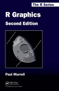
All of the functions in Chapter 6 that produce graphical output also produce graphical objects, or grobs, representing that output. For example, the following code produces a number of circles as output (see the left panel in Figure 7.1).
Modifying a circle grob. The left panel shows the output produced by a call to grid.circle(), the middle panel shows the result of using grid.edit() to modify the colors of the circles, and the right panel shows the result of using grid.remove() to delete the circles.
> grid.circle(name="circles", x=seq(0.1, 0.9, length=40),
y=0.5 + 0.4*sin(seq(0, 2*pi, length=40)),
r=abs(0.1*cos(seq(0, 2*pi, length=40))))
As well as drawing the circles, this code produces a circle grob, an object of class "circle", which contains information describing the circles that have been drawn. Importantly, this grob has been given a name, in this case "circles".
The grid system maintains a display list, a record of all viewports and grobs drawn on the current page, and the object that grid.circle() created is stored on this display list. This means that it can be accessed to obtain a copy, to modify the output, or even to remove it altogether. The grob has been given the name "circles" to make it easy to identify on the display list.
In the following code, the call to grid.get() obtains a copy of the circle object. This can be useful for inspecting the elements of a scene.
> grid.get("circles")
circle[circles]
The following call to grid.edit() modifies the output by editing the circle object to change the colors used for drawing the circles (see the middle panel of Figure 7.1). In this case, the gp component of the circle grob is being modified. Typically, most arguments that can be specified when first drawing output can also be used when editing output.
> grid.edit("circles",
gp=gpar(col=gray(c(1:20*0.04, 20:1*0.04))))
The next call below, to the grid.remove() function, deletes the output by removing the circle object from the display list (see the right panel of Figure 7.1).
> grid.remove("circles")
In each of these examples, the grob has been specified by giving its name ("circles"). Other standard arguments to these functions are discussed in the next section.
Any output produced by grid functions can be interacted with in this way, including output from lattice and ggplot2 functions (see Sections 7.7 and 7.8).
It is possible to disable the grid display list, using the grid.display.list() function, in which case no grobs are stored, so these sorts of manipulations are no longer possible.
7.1.1 Standard functions and arguments
The complete set of functions that provide the ability to interact with grobs is shown in Table 7.1.
Functions for working with grobs. Functions of the form grid.*() access and destructively modify grobs on the grid display list and affect graphical output. Functions of the form *Grob() work with user-level grobs and return grobs as their values (they have no effect on graphical output).
Function to Work with Output |
Description |
Function to Work with grobs |
|---|---|---|
grid.get() |
Returns a copy of one or more grobs |
getGrob() |
grid.edit() |
Modifies one or more grobs |
editGrob() |
grid.add() |
Adds a grob to one or more grobs |
addGrob() |
grid.remove() |
Removes one or more grobs |
removeGrob() |
grid.set() |
Replaces one or more grobs |
setGrob() |
All of the functions for working with graphical output require a grob name as the first argument, to identify which grob to work with. This name will be treated as a regular expression if the grep argument is TRUE. If the global argument is TRUE then all matching grobs on the display list (not just the first) will be accessed or modified.
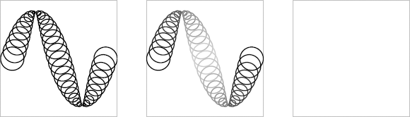
The following code provides a simple example. Eight concentric circle grobs are drawn, with the first, third, fifth, and seventh circles named "circle.odd" and the second, fourth, sixth, and eighth circles named "circle.even". The circles are initially drawn with decreasing shades of gray (see the left panel of Figure 7.2).
Editing grobs using grep and global in grid.edit(). The left-hand panel shows eight separate concentric circles, with names alternating between "circle.odd" and "circle.even", filled with progressively lighter shades of gray. The middle panel shows the use of the global argument to change the fill for all circles named "circle.odd" to black. The right-hand panel shows the use of the grep and global arguments to change all circles whose names match the pattern "circle" (all of the circles) to have a light gray fill and a gray border.
> suffix <- c("even", "odd")
> for (i in 1:8)
grid.circle(name=paste("circle.", suffix[i %% 2 + 1],
sep=""),
r=(9 - i)/20,
gp=gpar(col=NA, fill=gray(i/10)))
The following call to grid.edit() makes use of the global argument to modify all grobs named "circle.odd" and change their fill color to a very dark gray (see the middle panel of Figure 7.2).
> grid.edit("circle.odd", gp=gpar(fill="gray10"),
global=TRUE)
A second call to grid.edit(), below, makes use of both the grep argument and the global argument to modify all grobs with names matching the pattern "circle" (all of the circles) and change their fill color to a light gray and their border color to a darker gray (see the right panel of Figure 7.2).
> grid.edit("circle", gp=gpar(col="gray", fill="gray90"),
grep=TRUE, global=TRUE)
There are convenience functions grid.gget() and grid.gedit() that have the grep and global arguments set to TRUE by default.
In summary, as long as the name of a grob is known, it is possible to access that grob using grid.get(), modify it using grid.edit(), or delete it using grid.remove().
The function grid.ls() is useful for producing a list of all grobs in the current scene, as shown by the following code.
> grid.ls()
circle.odd
circle.even
circle.odd
circle.even
circle.odd
circle.even
circle.odd
circle.even
This function is described in more detail in Section 8.4.
7.2 Grob lists, trees, and paths
As well as basic grobs, it is possible to work with a list of grobs (a gList) or several grobs combined together in a tree-like structure (a gTree). A gList is just a list of several grobs (produced by the function gList()). A gTree is a grob that can contain other grobs. Examples are the xaxis and yaxis grobs. This section looks at how to work with gTrees.
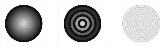
An xaxis grob contains a high-level description of an axis, plus several child grobs representing the lines and text that make up the axis (see Figure 7.3).
The structure of a gTree. A diagram of the structure of an xaxis gTree. There is the xaxis gTree itself (here given the name "xaxis1") and there are its children: a lines grob named "major", another lines grob named "ticks", and a text grob named "labels".
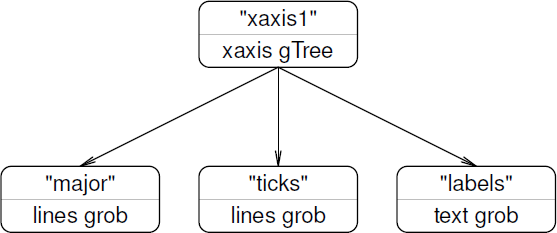
The following code draws an x-axis and creates an xaxis grob on the display list (see the left panel of Figure 7.4). The grid.ls() function shows that the axis1 grob has three child grobs.

Editing a gTree. The left-hand panel shows a basic x-axis, the middle panel shows the effect of editing the at component of the x-axis (all of the tick marks and labels have changed), and the right-hand panel shows the effect of editing the rot component of the "labels" child of the x-axis (only the angle of rotation of the labels has changed).
> grid.xaxis(name="axis1", at=1:4/5)
> grid.ls()
axis1
major
ticks
labels
The hierarchical structure of gTrees makes it possible to interact with both a high-level description, as provided by the xaxis grob, and a low-level description, as provided by the children of the gTree. The following code demonstrates an interaction with the high-level description of an xaxis grob. The xaxis gTree contains components describing where to put tick marks on the axis and whether to draw labels and so on. The code below shows the at component of an xaxis grob being modified. The xaxis grob is designed so that it modifies its children to match the new high-level description so that only three ticks are now drawn (see the middle panel of Figure 7.4).
> grid.edit("axis1", at=1:3/4)
It is also possible to access the children of a gTree. In the case of an xaxis, there are three children: a lines grob with the name "major"; another lines grob with the name "ticks"; and a text grob with the name "labels". Any of these children can be accessed by specifying the name of the xaxis grob and the name of the child in a grob path (gPath). A gPath is like a viewport path (see Section 6.5.3) — it is just a concatenation of several grob names. The following code shows how to access the "labels" child of the xaxis grob using the gPath() function to specify a gPath. The gPath specifies the child called "label" in the gTree called "axis1". The labels are rotated to 45 degrees (see the right panel of Figure 7.4).
> grid.edit(gPath("axis1", "labels"), rot=45)
It is also possible to specify a gPath directly as a string, for example "axis1::labels", but this is only recommended for interactive use.
7.2.1 Graphical parameter settings in gTrees
Just like any other grob, a gTree can have graphical parameter settings associated with it via a gp component. These settings affect all graphical objects that are children of the gTree, unless the children specify their own graphical parameter setting. In other words, the graphical parameter settings for a gTree modify the implicit graphical context for the children of the gTree (see page 194).
The following expression demonstrates this rule. The gp component of an xaxis grob sets the drawing color to be "gray". This means that all of the children of the xaxis — the lines and labels — will be drawn gray.
> grid.xaxis(gp=gpar(col="gray"))
Another example of this behavior is given in Section 7.3 and the role of the gp component in the drawing behavior of gTree objects is described in more detail in Section 8.3.4.
7.2.2 Viewports as components of gTrees
Just like any other grob, a gTree can have a viewport (or viewport tree, or viewport path, etc.) associated with it via a vp component. This viewport is pushed before the gTree is drawn and popped afterward (see Section 6.5.4). This means that the children of a gTree are drawn within the drawing context defined by the viewport in the vp slot of the gTree (see page 199).
The following code demonstrates this rule. The vp component of an xaxis grob specifies a viewport in the top half of the page. This means that the children of the xaxis are positioned relative to that viewport.
> grid.xaxis(vp=viewport(y=0.75, height=0.5))
An example of this behavior is given in Section 7.3 and the role of the vp component in the drawing behavior of gTree objects is described in more detail in Sections 8.3.4 and 8.3.7.
7.2.3 Searching for grobs
This section provides details about how grob names and gPaths are used to find a grob.
Grobs are stored on the grid display list in the order that they are drawn. When searching for a matching name, the functions in Table 7.1 search the display list from the beginning. This means that if there are several grobs whose names are matched, they will be found in the order that they were drawn.
Furthermore, the functions perform a depth-first search. This means that if there is a gTree on the display list, and its name is not matched, then its children are searched for a match before any other grobs on the display list are searched.
The name to search for can be given as a gPath, which makes it possible to explicitly specify a particular child grob of a particular gTree. For example, "axis1::labels" specifies a grob called "labels" that must have a parent called "axis1".
The argument strict controls whether a complete match must be found. By default, the strict argument is FALSE, so in the previous example, the "labels" child of "axis1" could have been accessed with the expression grid.get("labels"). On the other hand, if strict is set to TRUE, then simply specifying "labels" results in no match because there is no top-level grob with the name "labels", as shown by the following code.
> grid.edit("labels", strict=TRUE, rot=45)
Error in
editDLfromGPath(gPath, specs, strict, grep, global, redraw) :
'gPath' (labels) not found
7.3 Working with graphical objects off-screen
Chapter 6 described grid functions that draw graphical output on the page or screen. All of those functions also create grobs representing the drawing and those grobs are stored on the grid display list.
It can also be useful to create a grob without producing any output. This section describes how to use grid to produce graphical objects (without drawing them). There are functions to create grobs, functions to combine them and to modify them, and the grid.draw() function to draw them.
For each grid function that produces graphical output, there is a counterpart that produces a graphical object and no graphical output. For example, the counterpart to grid.circle() is the function circleGrob() (see Table 6.1). Similarly, for each function that works with grobs on the grid display list, there is a counterpart for working with grobs off-screen. For example, the counterpart to grid.edit() is editGrob() (see Table 7.1).
The following example demonstrates the process of creating a grob and working with the grob without drawing it. The code below draws a rectangle that is as wide as a text grob, but the text is not drawn. The function textGrob() produces a text grob, but does not draw it.
> grid.rect(width=grobWidth(textGrob("Some text")))
It can be useful to create a grob and modify it before producing any graphical output (i.e., only draw the final result). The following code creates an axis and modifies the font face for the labels to italic before drawing the axis. The function grid.draw() is used to produce graphical output from a grob.
> ag <- xaxisGrob(at=1:4/5)
> ag <- editGrob(ag, "labels", gp=gpar(fontface="italic"))
> grid.draw(ag)
Another example of working with grobs is in the construction of gTrees. In its simplest form, a gTree is just a grouping of several grobs (more complex gTree creation is discussed later in Section 8.3).
By grouping several grobs together as a single object, the grobs can be dealt with as a single object. For example, it becomes possible to edit the graphical context for all of the grobs at once, or define the drawing context for all of the grobs at once.
When a gTree is drawn, any viewports in its vp component are pushed, any settings in its gp component are enforced, and then its children are all drawn. This means that the vp and gp components of a gTree affect where and how the children of the gTree are drawn (see Sections 7.2.1 and 7.2.2).
As an example, a boxed-text object can be created by grouping a "rect" grob and a "text" grob together as children of a gTree. This allows us to modify the color of both the rectangle and the text by modifying these features in the gTree. Similarly, it is possible to locate both the rectangle and the text by defining a viewport for the gTree.
The following code uses the gTree() function to create a gTree that groups a "rect" grob and a "text" grob together. There is no graphical output produced from this code. It only creates graphical objects.
> tg <- textGrob("sample text")
> rg <- rectGrob(width=1.1*grobWidth(tg),
height=1.3*grobHeight(tg))
> boxedText <- gTree(children=gList(tg, rg))
It is now easy to produce output including both the rectangle and the text by drawing variations on the boxedText grob, as demonstrated by the following code.
The first call simply draws the plain boxedText, which is drawn in black (see the left panel of Figure 7.5).
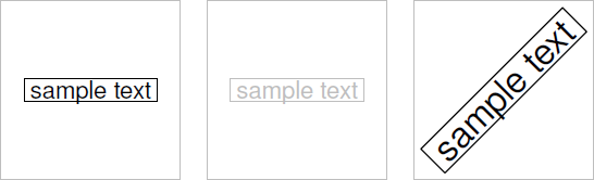
Using a gTree to group grobs. The left-hand panel shows a boxed text object (which is a combination of a piece of text and a rectangle). The middle panel shows how changes to the color settings in the boxed text object propagate to the components (both the text and rectangle turn gray). The right-hand panel shows a more dramatic demonstration of the same idea as, in this case, the font size of the boxed text is modified and it is drawn within a rotated viewport.
> grid.draw(boxedText)
The second call draws a modified boxedText with the drawing color set to gray (see the middle panel of Figure 7.5).
> grid.draw(editGrob(boxedText, gp=gpar(col="gray")))
The final call draws another modification of the boxedText, this time in a rotated viewport and with a larger font (see the right panel of Figure 7.5).
> grid.draw(editGrob(boxedText, vp=viewport(angle=45),
gp=gpar(fontsize=18)))
7.3.1 Capturing output
In the example in the previous section, several grobs are created off-screen and then grouped together as a gTree, which allows the collection of grobs to be dealt with as a single object.
It is also possible first to draw several grobs and then to group them. The grid.grab() function does this by generating a gTree from all of the grobs in the current page of output. This means that output can be captured even from a function that produces very complex output (lots of grobs), such as a lattice plot. For example, the following code draws a lattice plot, then creates a gTree containing all of the grobs in the plot.
> bwplot(rnorm(10))
> bwplotTree <- grid.grab()
The grid.grab() function actually captures all of the viewports in the current scene as well as the grobs, so drawing the gTree, as in the following code, produces exactly the same output as the original plot.
> grid.newpage()
> grid.draw(bwplotTree)
Another function, grid.grabExpr() allows complex output to be captured off-screen. This function takes an R expression and evaluates it. Any drawing that occurs as a result of evaluating the expression does not produce any output, but the grobs that would be produced are captured anyway.
The following code provides a simple demonstration. Here a lattice plot is captured without drawing any output.*
> grid.grabExpr(print(bwplot(rnorm(10))))
gTree[GRID.gTree.100]
Both the grid.grab() and grid.grabExpr() functions attempt to create a gTree in a sophisticated way so that it is easier to work with the resulting gTree. Unfortunately, this will not always produce a gTree that will exactly replicate the original output. These functions issue warnings if they detect a situation where output may not be reproduced correctly, and there is a wrap argument that can be used to force the functions to produce a gTree that is less sophisticated, but is guaranteed to replicate the original output.
7.4 Placing and packing grobs in frames
It can be useful to position the components of a plot in a way that leaves sufficient room for labels or legends. The "grobwidth" and "grobheight" coordinate systems provide a way to determine the size of a grob and can be used to achieve this sort of arrangement of components by, for example, allocating appropriate regions within a layout.
The following code demonstrates this idea. First of all, some grobs are created to use as components of a scene. The first grob, label, is a simple text grob. The second grob, gplot, is a gTree containing a rect grob, a lines grob, and a points grob that provide a simple representation of time-series data. The gplot has a viewport in its vp component and the rectangle and lines are drawn within that viewport.
> label <- textGrob("A
Plot
Label ",
x=0, just="left")
> x <- seq(0.1, 0.9, length=50)
> y <- runif(50, 0.1, 0.9)
> gplot <-
gTree(
children=gList(rectGrob(gp=gpar(col="gray60",
fill="white")),
linesGrob(x, y),
pointsGrob(x, y, pch=16,
size=unit(1.5, "mm"))),
vp=viewport(width=unit(1, "npc") - unit(5, "mm"),
height=unit(1, "npc") - unit(5, "mm")))
The next piece of code defines a layout with two columns. The second column of the layout has its width determined by the width of the label grob created above. The first column will take up whatever space is left over.
> layout <- grid.layout(1, 2,
widths=unit(c(1, 1),
c("null", "grobwidth"),
list(NULL, label)))
Now some drawing can occur. A viewport is pushed with the layout defined above, then the label grob is drawn in the second column of this layout, which is exactly the right width to contain the text, and the gplot gTree is drawn in the first column (see Figure 7.6).
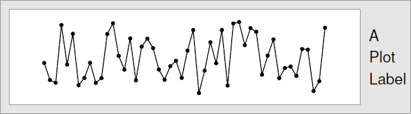
Packing grobs by hand. The scene was created using a frame object, into which the time-series plot (consisting of a rectangle, lines, and points) was packed. The text was then packed on the right-hand side, which meant that the time series plot was allocated less room in order to leave space for the text.
> pushViewport(viewport(layout=layout))
> pushViewport(viewport(layout.pos.col=2))
> grid.draw(label)
> popViewport()
> pushViewport(viewport(layout.pos.col=1))
> grid.draw(gplot)
> popViewport(2)
The grid package provides a set of functions that make it more convenient to arrange grobs like this so that they allow space for each other. The function grid.frame(), and its off-screen counterpart frameGrob(), produce a gTree with no children. Children are added to the frame using the grid.pack() function and the frame makes sure that enough space is allowed for the child when it is drawn. Using these functions, the previous example becomes simpler, as shown by the following code (the output is the same as Figure 7.6).
The big difference is that there is no need to specify a layout as an appropriate layout is calculated automatically.
The first call creates an empty frame. The second call packs gplot into the frame; at this stage, gplot takes up the entire frame. The third call packs the text label on the right-hand side of the frame; enough space is made for the text label by reducing the space allowed for the rectangle.
> grid.frame(name="frame1")
> grid.pack("frame1", gplot)
> grid.pack("frame1", label, side="right")
There are many arguments to grid.pack() for specifying where to pack new grobs within a frame. There is also a dynamic argument to specify whether the frame should reallocate space if the grobs that have been packed in the frame are modified.
Unfortunately, packing grobs into a frame like this becomes quite slow as more grobs are packed, so it is most useful for very simple arrangements of grobs or for interactively constructing a scene. An alternative approach, which is a little more work, but still more convenient than dealing directly with pushing and popping viewports (and can be made dynamic like packing), is to place grobs within a frame that has a predefined layout. The following code demonstrates this approach. This time, the frame is initially created with the desired layout as defined above, then the grid.place() function is used to position grobs within specific cells of the frame layout.
> grid.frame(name="frame1", layout=layout)
> grid.place("frame1", gplot, col=1)
> grid.place("frame1", label, col=2)
7.4.1 Placing and packing off-screen
In the previous two examples, the screen is redrawn each time a grob is packed into the frame. It is more typical to create a frame and pack or place grobs within it off-screen and only draw the frame once it is complete. The following code demonstrates the use of the frameGrob() and placeGrob() functions to achieve the same end result as shown in Figure 7.6, doing all of the construction of the frame off-screen.
> fg <- frameGrob(layout=layout)
> fg <- placeGrob(fg, gplot, col=1)
> fg <- placeGrob(fg, label, col=2)
> grid.draw(fg)
The function packGrob() is the off-screen counterpart of grid.pack().
7.5 Other details about grobs
This section describes some important extra details about the calculation of grob sizes and the editing of graphical contexts.
7.5.1 Calculating the sizes of grobs
As described in Section 6.3.2, the "grobwidth" and "grobheight" units, and the grobWidth() and grobHeight() functions, provide a way to determine the size of a grob. This section provides some more details about the correct usage of these units.
The most important point is that the size of a grob is always calculated relative to the current geometric and graphical context. The following code demonstrates this point. First of all, a text grob and a rect grob are created, and the dimensions of the rect grob are based on the dimensions of the text.*
> tg1 <- textGrob("Sample")
> rg1 <- rectGrob(x=rep(0.5, 2),
width=1.1*grobWidth(tg1),
height=1.3*grobHeight(tg1),
gp=gpar(col=c("gray60", "white"),
lwd=c(3, 1)))
Next, these two grobs are drawn in three different settings. In the first setting, the rectangle and the text are drawn in the default geometric and graphical context and the rectangle bounds the text (see the left panel of Figure 7.7).
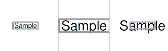
Calculating the size of a grob. In the left-hand panel, a text grob and a separate rect grob, the size of which is calculated to be the size of the text grob, are drawn together. In the middle panel, these objects are drawn together in a viewport with a larger font size, so they are both larger. In the right-hand panel, only the text is drawn in a viewport with a larger font size, so only the text is larger. The rectangle calculates the size of the text in a different font context.
> grid.draw(tg1)
> grid.draw(rg1)
In the second setting, the grobs are both drawn within a viewport that has cex=2. Both the text and the rectangle are drawn bigger (the calculation of the "grobwidth" and "grobheight" units takes place in the same context as the drawing of the text grob; see the middle panel of Figure 7.7).
> pushViewport(viewport(gp=gpar(cex=2)))
> grid.draw(tg1)
> grid.draw(rg1)
> popViewport()
In the third setting, the text grob is drawn in a different context than the rectangle, so the rectangle’s size is “wrong” (see the right panel of Figure 7.7).
> pushViewport(viewport(gp=gpar(cex=2)))
> grid.draw(tg1)
> popViewport()
> grid.draw(rg1)
A related issue arises with the use of grob names when creating a "grobwidth" or "grobheight" unit (see Section 6.3.2). The following code provides a simple example.
A text grob and two rect grobs are created, with the dimensions of both rectangles based upon the dimensions of the text. One rectangle, rg1, uses a copy of the text grob in the calls to grobWidth(), and grobHeight(). The other rectangle, rg2, just uses the name of the text grob, "tg1".
> tg1 <- textGrob("Sample", name="tg1")
> rg1 <- rectGrob(width=1.1*grobWidth("tg1"),
height=1.3*grobHeight("tg1"),
gp=gpar(col="gray60", lwd=3))
> rg2 <- rectGrob(width=1.1*grobWidth(tg1),
height=1.3*grobHeight(tg1),
gp=gpar(col="white"))
When these rectangles and text are initially drawn, both rectangles frame the text correctly (see the left panel of Figure 7.8).
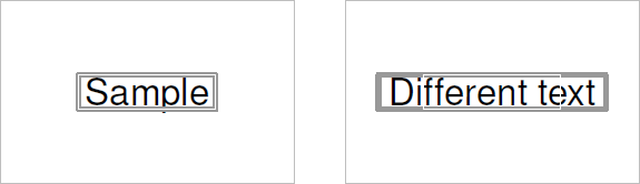
Grob dimensions by reference. In the left-hand panel there are three grobs: one text grob and two rect grobs. The sizes of both rect grobs are calculated from the text grob. The difference is that the white rectangle is related to the text by value and the dark gray rectangle is related to the text by reference. The right-hand panel shows what happens when the text grob is edited. Only the dark gray, by-reference, rectangle gets resized.
> grid.draw(tg1)
> grid.draw(rg1)
> grid.draw(rg2)
However, if the text grob is modified, as shown below, only the rectangle rg1 (the dark gray rectangle) will be updated to correspond to the new dimensions of the text (see the right panel of Figure 7.8).
> grid.edit("tg1", grep=TRUE, global=TRUE,
label="Different text")
With this approach, "grobwidth" and "grobheight" units are still evaluated in the current geometric and graphical context, but in addition, only grobs that have previously been drawn can be referred to. For example, drawing the rectangle rg1 before drawing the text tg1 will not work because there is no drawn grob named "tg1" from which a size can be calculated.
> grid.newpage()
> grid.draw(rg1)
Error in function (name) :
Grob 'tg1' not found
7.5.2 Calculating the positions of grobs
In addition to being able to query a grob about its dimensions, it is also possible to query a grob about its location, using "grobx" and "groby" units, or the grobX() and grobY() functions.
Locations are calculated relative to the current geometric and graphical context, just like widths and heights, so all of the warnings from the previous section also apply here.
The grob locations are positions on the border of a grob, given by an angle (relative to the “center” of the grob). The following code shows a simple example usage (see Figure 7.9). A small dot is drawn on the left and a text label, with a surrounding box, is drawn on the right. The box grob is named "labelbox".

Calculating grob locations. The line segment is drawn from an explicit (x, y) start location to an end location that is calculated using grobX() to give the left edge of the box surrounding the text.
> grid.circle(.25, .5, r=unit(1, "mm"),
gp=gpar(fill="black"))
> grid.text("A label", .75, .5)
> grid.rect(.75, .5,
width=stringWidth("A label") + unit(2, "mm"),
height=unit(1, "line"),
name="labelbox")
A line segment, with an arrow, is now drawn between the dot and the left edge of the box, using the grobX() function to determine the location of the left edge of the box.
> grid.segments(.25, .5,
grobX("labelbox", 180), .5,
arrow=arrow(angle=15, type="closed"),
gp=gpar(fill="black"))
The next example demonstrates a more complex use. This replicates an example from Figure 3.18 and demonstrates a possible use for “null” grobs.
First of all, two viewports are created, one in the top half of the page and one in the bottom half.
> vptop <- viewport(width=.9, height=.4, y=.75,
name="vptop")
> vpbot <- viewport(width=.9, height=.4, y=.25,
name="vpbot")
> pushViewport(vptop)
> upViewport()
> pushViewport(vpbot)
> upViewport()
Now a rectangle and a line through some data are drawn in each viewport.
> grid.rect(vp="vptop")
> grid.lines(1:50/51, runif(50), vp="vptop")
> grid.rect(vp="vpbot")
> grid.lines(1:50/51, runif(50), vp="vpbot")
The next step does not draw anything, it just locates several null grobs at specific locations, two in the top viewport and two in the bottom viewport.
> grid.null(x=.2, y=.95, vp="vptop", name="tl")
> grid.null(x=.4, y=.95, vp="vptop", name="tr")
> grid.null(x=.2, y=.05, vp="vpbot", name="bl")
> grid.null(x=.4, y=.05, vp="vpbot", name="br")
Finally, a polygon is drawn that spans both viewports. The first two vertices of the polygon are calculated from the positions of the two null grobs in the top viewport and the second two vertices of the polygon are calculated from the positions of the two null grobs in the bottom viewport.
> grid.polygon(unit.c(grobX("tl", 0),
grobX("tr", 0),
grobX("br", 0),
grobX("bl", 0)),
unit.c(grobY("tl", 0),
grobY("tr", 0),
grobY("br", 0),
grobY("bl", 0)),
gp=gpar(col="gray", lwd=3))
The final result is shown in Figure 7.10.
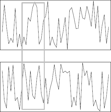
Calculating null grob locations. The two line plots are drawn in separate viewports. The thick gray rectangle is drawn relative to the locations of four null grobs, two of which are located in the top viewport and two of which are located in the bottom viewport.
7.5.3 Editing graphical context
When a grob is edited using grid.edit() or editGrob(), the modification of a gp component is treated as a special case. Only the graphical parameters that are explicitly given new settings are modified. All other settings remain untouched. The following code provides a simple example.
A circle is drawn with a gray fill color (see the left panel of Figure 7.11), then the border of the circle is made thick (see the middle panel of Figure 7.11) and the fill color remains the same. Finally, the border is changed to a dashed line type, but it stays thick (and the fill remains gray — see the right panel of Figure 7.11).
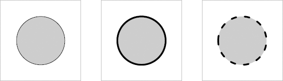
Editing the graphical context. The left-hand panel shows a circle with a solid, thin black border and a gray fill. The middle panel shows the effect of making the border thicker. The important point is that the other features of the circle are not affected (the border is still solid and the fill is still gray). The right-hand panel shows another demonstration of the same idea, with the border now drawn dashed (but the border is still thick and the fill is still gray).
> grid.circle(r=0.3, gp=gpar(fill="gray80"),
name="mycircle")
> grid.edit("mycircle", gp=gpar(lwd=5))
> grid.edit("mycircle", gp=gpar(lty="dashed"))
7.6 Saving and loading grid graphics
The best way to create a persistent record of a grid plot is to record in a text file the R code that was used to create the plot. The code can then be run again, e.g., using source(), to reproduce the output.
It is also possible to save grobs in R’s binary format using the save() function. The grobs can then be loaded, using load(), and redrawn using grid.draw(). For the purpose of saving an entire scene, it may be more useful to save and load a gTree created by the grid.grab() function (see Section 7.3.1).
A possible danger with saving a grid grob is that methods specific to that grob are not automatically recorded, so the grob may not behave correctly when loaded into a different session. This will only be an issue for grobs that are not predefined by grid (see Chapter 8, particularly Section 8.3).
7.7 Working with lattice grobs
The output from a lattice function is fundamentally just a collection of grid viewports and grobs. Section 6.8 described some examples of making use of the grid viewports that are set up by a lattice plot to add extra output. This section looks at some examples of working with the grobs that are created by a lattice plot.
The following code creates a lattice scatterplot to work with.
> angle <- seq(0, 2*pi, length=21)[-21]
> x <- cos(angle)
> y <- sin(angle)
> xyplot(y ~ x, aspect=1,
xlab="displacement",
ylab="velocity")
The grid.ls() function shows the set of graphical primitives that have been created for this plot.
> grid.ls()
GRID.rect.156
plot_01.xlab
plot_01.ylab
GRID.segments.157
GRID.segments.158
GRID.text.159
GRID.segments.160
GRID.text.161
GRID.segments.162
GRID.points.163
GRID.rect.164
The grobs created by other people’s functions will not necessarily provide useful names for all components that are drawn, but in this case, it is easy to spot which components provide the x-axis label and y-axis label for the plot.
The following code edits the axis labels to change the font to a "mono" family and to position the labels at the ends of the axes (see Figure 7.12).
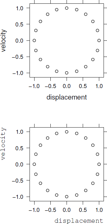
Editing the grobs in a lattice plot. The top plot is an initial scatterplot produced using the lattice function xyplot(). The bottom plot shows the effect of editing the grid text grobs that represent the labels on the plot (the labels are relocated at the ends of the axes and are drawn in a monospace font).
> grid.edit("[.]xlab$", grep=TRUE,
x=unit(1, "npc"), just="right",
gp=gpar(fontfamily="mono"))
> grid.edit("[.]ylab$", grep=TRUE,
y=unit(1, "npc"), just="right",
gp=gpar(fontfamily="mono"))
Other grob operations are also possible. For example, the following code removes the labels from the plot.
> grid.remove(".lab$", grep=TRUE, global=TRUE)
Finally, it is possible to group all of the grobs from a lattice plot together using grid.grab(). This creates a gTree that can then be used as a component in creating another picture.
7.8 Working with ggplot2 grobs
Like lattice, ggplot2 creates lots of grid grobs when it draws a plot and these grobs can be manipulated using grid functions.
The following code uses ggplot2 to create a scatterplot with a linear model line of best fit.
> ggplot(mtcars2, aes(x=disp, y=mpg)) +
geom_point() +
geom_smooth(method=lm)
The next code navigates down to the plot region and queries the grob that represents the line of best fit, using grobX() and grobY(), to determine a location on the line. This location is used to draw an arrow that points from a text label to the line of best fit (see Figure 7.13).
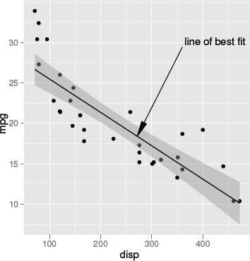
Working with ggplot2 grobs. A ggplot2 scatterplot is drawn and then a line is added with an end point that is calculated from the grob that represents the smooth line on the plot.
> downViewport("panel-3-3")
> sline <- grid.get(gPath("smooth", "polyline"),
grep=TRUE)
> grid.segments(.7, .8,
grobX(sline, 45), grobY(sline, 45),
arrow=arrow(angle=10, type="closed"),
gp=gpar(fill="black"))
> grid.text("line of best fit", .71, .81,
just=c("left", "bottom"))
Determining the name of the correct grob in this example required an inspection of the output from grid.ls(). Section 8.4 provides more examples of how to explore grid grobs and viewports.
Chapter summary
As well as producing graphical output, all grid functions create grobs (graphical objects) that contain descriptions of what has been drawn. These grobs may be accessed, modified, and even removed, and the graphical output will be updated to reflect the changes.
There are also grid functions for creating grobs without producing any graphical output. A complete description of a plot can be produced by creating, modifying, and combining grobs off-screen.
A gTree is a grob that can have other grobs as its children. A gTree can be useful for grouping grobs and for providing a high-level interface to a group of grobs.
The lattice and ggplot2 plotting functions generate large numbers of grid grobs. These grobs may be manipulated just like any other grobs to access, edit, and delete parts of a ggplot2 or lattice plot.
*The expression must explicitly print() the lattice plot because otherwise nothing would be drawn (see Section 4.1).
*The rect grob draws two rectangles: one thick and dark gray, one white and thin.