Chapter 15
Node-and-edge Graphs
Chapter preview
This chapter describes how to produce node-and-edge graphs with R. Node-and-edge graphs are a special case because producing a graph visualization usually requires special algorithms to determine a useful arrangement of the nodes on a page. Several packages are described that provide this facility, notably Rgraphviz and igraph. This chapter also describes how to draw more regular node-and-edge diagrams in R.
The main graphics systems in R, traditional, lattice, and ggplot2, are all focused on producing graphs in the sense of statistical plots. Another common meaning of the term “graph” is a set of nodes with edges connecting them. This chapter describes packages that are focused on producing images of this sort of node-and-edge graph.
There are three important steps involved in producing an image of a node-and-edge graph:
- An object representing the graph must be created.
- A layout must be generated for the graph, which provides a description of where all of the nodes and edges should be drawn.
- The graph needs to be rendered, which involves drawing the information in the graph representation, such as the names of the nodes, at the locations specified in the layout.
15.1 Creating graphs
A graph consists of a set of nodes and a set of edges, where each edge is a connection between any two nodes. This information about a graph can be represented in R in any number of ways and different packages provide different solutions. However, many of the packages that work with graphs, particularly those that produce graph visualizations, depend on graph representations provided by the graph package.
15.1.1 The graph package
The graph package provides two simple ways to specify a graph.
> library(graph)
The graph can be described in terms of explicit node names and an explicit list of edges between nodes, a "graphNEL" object, or in terms of an adjacency matrix, a "graphAM" object, where there is an edge between node i and node j if element (i, j) of the matrix has the value 1.
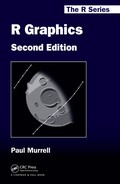
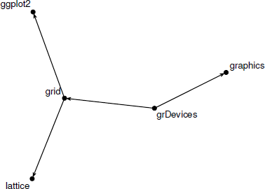
The following code shows how to create a simple graph from a vector of node names and a list of edges. This graph shows the relationships between the five core graphics packages in R. A visualization of this simple graph is shown in Figure 15.1. Notice that the graph is directed, so edges go only one way between two nodes.
A simple node-and-edge graph consisting of five nodes. This shows the relationship between the core graphics functions in R. This graph has been rendered by the Rgraphviz package.
> nodes <- c("grDevices", "graphics", "grid",
"lattice", "ggplot2")
> edgeList <-
list(grDevices=list(edges=c("graphics", "grid")),
graphics=list(),
grid=list(edges=c("lattice", "ggplot2")),
lattice=list(),
ggplot2=list())
> simpleGNEL <- new("graphNEL",
nodes=nodes,
edgeL=edgeList,
edgemode="directed")
The following code shows an equivalent graph defined via an adjacency matrix.
> adjMat <- rbind(grDevices=c(0, 1, 1, 0, 0),
graphics=rep(0, 5),
grid=c(0, 0, 0, 1, 1),
lattice=rep(0, 5),
ggplot2=rep(0, 5))
> simpleGAM <- new("graphAM", adjMat, edgemode="directed")
For small graphs, it is feasible to specify the nodes and edges by hand as in the above examples, but for larger graphs the set of nodes and the edge list, or the adjacency matrix, can be generated programmatically.
Alternatively, an external description of a graph in the GXL* format can be read into R, as a "graphNEL" object, using the fromGXL() function. For example, Figure 15.2 shows a file, simplegraph.gxl, containing GXL code for the simple graph example above and the following code creates a "graphNEL" object from that file.

A simple GXL file that describes a graph consisting of five nodes. This is the graph that is drawn in Figure 15.1.
> simpleGNEL <- fromGXL(file("simplegraph.gxl"))
The graph package also provides functions for manipulating graphs. For example, the subGraph() function can be used to extract a subgraph from a larger graph and the leaves() function can be used to determine the leaf nodes of a graph. In the following code, subGraph() is used to extract just the grid-related nodes from simpleGNEL and leaves() is used to find the leaf nodes of simpleGNEL.
> smallGNEL <- subGraph(c("grid", "lattice", "ggplot2"),
simpleGNEL)
> smallGNEL
A graphNEL graph with directed edges
Number of Nodes = 3
Number of Edges = 2
> leaves(simpleGNEL, "out")
[1] "graphics" "lattice" "ggplot2"
15.2 Graph layout and rendering
Having generated a representation of a graph, drawing the graph requires deciding where to draw nodes and edges, the layout step, and then drawing the nodes and edges at those locations, the rendering step.
For very simple graphs, it may be feasible or desirable to position the nodes and edges by hand. That scenario is dealt with in Section 15.4. This section addresses the more complex problem of positioning graphs with numerous nodes and edges. In this case, some sort of layout algorithm must be employed.
Several packages implement graph layout algorithms, but the focus in this section is on the Rgraphviz package, which provides an interface to the graphviz software library.*
15.2.1 The Rgraphviz package
The Rgraphviz package is part of the Bioconductor project. This package provides both layout and rendering facilities for graphs that have been created using the graph package.
> library(Rgraphviz)
Rendering a graph is as simple as calling the generic plot() function with a "graphNEL" or "graphAM" object as the argument. The following code renders the simple graph introduced earlier to produce the result shown in Figure 15.1.
> plot(simpleGNEL)
This rendering uses the default layout algorithm for Rgraphviz, which is called dot. This algorithm places nodes in a hierarchical layout consisting of horizontal layers, tries to keep edges short, and tries to avoid edge crossings.
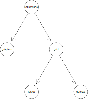
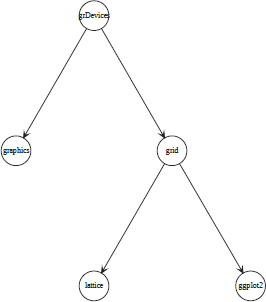
The second argument to this plot() method is the algorithm to use for laying out the graph. There are several options; the following code shows how to select a neato layout, which treats edges as if they are springs and finds a layout that balances the tension of the springs. Figure 15.3 shows the resulting layout for the simple graph.
Rendering a graph with Rgraphviz, using the neato layout algorithm. This should be compared with the graph layout in Figure 15.1, which used the default dot layout algorithm.
> plot(simpleGNEL, "neato")
The help page for "GraphvizLayouts" provides more information on the layout algorithms.
15.2.2 Graph attributes
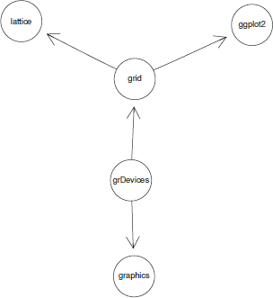
It is also possible to supply graph attributes, which affect the rendering of the graph. The following code demonstrates one way to do this, by supplying additional arguments to the call to plot(). In this case, the nodeAttrs and edgeAttrs arguments are used to modify the appearance of individual nodes and edges. The resulting graph is shown in Figure 15.4.
A simple graph rendered with Rgraphviz, but using graph attributes to modify the appearance of nodes and edges.
> plot(simpleGNEL,
edgeAttrs=list(lty=c(`grDevices~graphics`="solid",
`grDevices~grid`="solid",
`grid~lattice`="dashed",
`grid~ggplot2`="dashed")),
nodeAttrs=list(fillcolor=c(grDevices="white",
graphics="gray90", grid="gray90",
lattice="gray60", ggplot2="gray60")))
The help page for "GraphvizAttributes" provides a list of available attributes and their meanings. It may also help to refer to the documentation on the graphviz web site itself.*
15.2.3 Customization
The layout and rendering of graphs can be performed as separate steps. One way to do this, using the layoutGraph() and renderGraph() functions, is shown in the following code. The result is the same as Figure 15.1.
> layoutGNEL <- layoutGraph(simpleGNEL)
> renderGraph(layoutGNEL)
The usefulness of separating the steps like this is that an intermediate object, here layoutGNEL, is created with information about the arrangement of the nodes and edges.
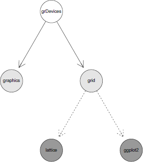
This leads to an alternative method of customizing the appearance of nodes and edges using functions like nodeRenderInfo() and edgeRenderInfo(). The following code modifies the background color for some nodes and the line style for some edges to create the same result as shown in Figure 15.4.
> nodeRenderInfo(layoutGNEL) <-
list(fill=c(graphics="gray90", grid="gray90",
lattice="gray60", ggplot2="gray60"))
> edgeRenderInfo(layoutGNEL) <-
list(lty=c(`grid~lattice`="dashed",
`grid~ggplot2`="dashed"))
Another option is to make use of the layout information in the intermediate object to add further drawing to a graph or even to take control of drawing the graph itself. For example, the plot() method for graph objects and the renderInfo() function are based on traditional graphics. Figure 15.5 shows an example where layoutGraph() was used to calculate node positions, then the resulting layout was rendered using grid. The code for this example is available on the book web site.
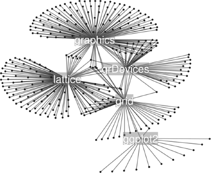
A more complex graph laid out using the neato layout algorithm. This graph has been created by using Rgraphviz to do the layout, but then grid to do the rendering. The graph has a node for all packages that directly depend on or import one of the core graphics packages in R (based on the state of CRAN on March 5, 2010).
15.2.4 Output formats
By rendering a graph using R, it is possible to produce output in any of the graphics formats that the R engine supports (see Chapter 9). However, those formats are purely for displaying a graph.
Another option is to save a graph in a format that facilitates further editing of the graph (using other software), for example in graphviz’s native dot format or the native format of a diagram editor such as xfig or dia.* The function toFile() provides several extra formats of this sort.
Yet another way to work is to use the toFile() function to call graphviz to perform not only the graph layout, but also the graph rendering, which in some cases may produce a higher-quality result compared to a rendering in R. For example, the following code produces a PDF file that has been both laid out and rendered by graphviz (see Figure 15.6). In this case, the agopen() function is used to lay out the graph and provide toFile() with the correct sort of R object that it requires.
> toFile(agopen(simpleGNEL, ""),
filename="Figures/graph-graphvizrender.pdf",
fileType="pdf")
15.2.5 Hypergraphs
The graph package only supports standard directed or undirected graphs, where an edge connects exactly two nodes. In a hypergraph, an edge can connect more than two nodes. The hypergraph and hyperdraw packages from the Bioconductor project provide some facilities for creating and rendering hypergraphs.
> library(hyperdraw)
The following code provides a simple example. A hypergraph is constructed using functions from the hypergraph package and then the graph is plotted using graphBPH() and a hypergraph plot() method from the hyperdraw package. The result is shown in Figure 15.7.
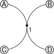
A simple hypergraph consisting of one hyperedge that connects one pair of nodes to another pair of nodes. This hypergraph has been rendered by the hyperdraw package.
> dh <- DirectedHyperedge(c("A", "B"), c("C", "D"))
> hg <- Hypergraph(LETTERS[1:4], list(dh))
> plot(graphBPH(hg))
15.3 Other packages
The combination of graph and Rgraphviz provides only one possible approach to drawing node-and-edge graphs in R. This section desribes several other packages that provide functions for creating and rendering graphs.
15.3.1 The igraph package
The igraph package provides a large set of functions both for creating graphs and for laying out and rendering graphs.
> library(igraph)
This package provides several convenient features for creating graphs. On one hand, there are functions that provide simple interfaces for creating the graph structure. For example, the graph() function accepts a numeric vector where each pair of values describes an edge. The following code creates the simple graph structure from Section 15.1.1.
> simpleIgraph <- graph(c(0, 1, 0, 2, 2, 3, 2, 4))
Another interface is provided by the graph.formula() function, which allows the edges to be specified using a special syntax. The following code creates the simple graph from Section 15.1.1.
> formulaIgraph <- graph.formula(grDevices -+ graphics,
grDevices -+ grid,
grid -+ lattice,
grid -+ ggplot2)
The igraph package also has a number of functions that generate regular or well-known graphs. For example, the graph.tree() function produces regular hierarchical graphs and the graph.full() function produces regular fully connected graphs (see Figure 15.8).
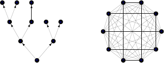
Two examples of regular graphs: a tree graph (left) and a fully connected graph (right).
> treeIgraph <- graph.tree(10)
> fullIgraph <- graph.full(10)
There is also the graph.famous() function for well-known “named” graphs, the graph.atlas() function to create one of the 1253 graphs from the book An Atlas of Graphs, and many more.
The igraph package also offers a wide variety of graph layout algorithms. For example, the layout.reingold.tilford() function performs a hierarchical layout similar to the dot algorithm of graphviz and the layout.spring() is in a similar spirit to the neato algorithm. In addition, the igraph package offers several more variations on the spring or force layout algorithm and layout.circle() to place all nodes on the circumference of a circle.
The sizing and labeling of graphs in the rendered output is less automated in igraph, but it is possible to control these features via functions such as set.vertex.attribute() and set.edge.attribute().
The existence of the igraph.to.graphNEL() function means that one fruitful approach is to make use of the igraph package to generate a graph and then convert it to something that Rgraphviz can render.
The igraph package has several other distinctive features. The tkplot() function provides an interactive editor, which can be used to click and drag individual nodes to fine tune the layout of a graph. There is also the function read.graph() to read a graph description from an external file in a variety of formats, plus the write.graph() function to save a graph in one of those formats.
15.3.2 The network package
The network package is part of the statnet suite of software packages for network analysis.* It provides the basic visualization functions for network objects.
This package is notable for supporting a very general concept of a graph. For example, it can cope with hypergraphs, where a single edge can connect more than two nodes, in addition to the standard graph where an edge connects exactly two nodes.
A graph may be created via the network() function, supplying the number of nodes and the graph edges as an adjacency matrix or as an “edge list”(actually a matrix, where each row specifies an edge). The following code creates the simple directed graph from previous sections.
> library(network)
> simpleNetwork <-
network(rbind(c(1, 2),
c(1, 3),
c(3, 4),
c(3, 5)),
vertex.attr=list(vertex.names=nodes))
The network package can also lay out and render graphs, though there are only a few layout algorithms available and the rendering style is different again from Rgraphviz and igraph. For example, node labels are drawn adjacent to nodes rather than within nodes.
A plot() method for "network" objects performs the layout and rendering. This function has many parameters to allow control over the appearance of the rendered graph, including mode, which controls the layout algorithm. The following code draws the simpleNetwork object (see Figure 15.9).
A simple network consisting of three nodes, with edge between nodes 1 and 2, between nodes 2 and 3, and between nodes 3 and 1. This network has been rendered by the network package.
> plot(simpleNetwork, mode="fruchtermanreingold",
vertex.col=1, displaylabels=TRUE)
One advantage of this package is that it does not depend on any third-party software to perform the graph layout.
Many other packages provide rendering of graphs or trees for particular areas of application. For example, the ape package provides a range of layout styles and flexible facilities for labeling nodes and edges of phylogenetic trees.
15.4 Diagrams
This section looks at drawing arrangements of nodes and edges when the positioning is more deliberate or does not require automating, such as in the production of flow charts.
15.4.1 The diagram and shape packages
The shape package provides functions for drawing a variety of geometric shapes and arrowheads and the diagram package provides functions for positioning shapes and drawing lines or curves between them. Together, these packages provide convenient functions for producing simple diagrams consisting of nodes and edges.
> library(diagram)
The function coordinates() provides a convenient way to calculate locations (on a zero-to-one scale) for a simple arrangement of nodes. Given a vector of n integers, this will calculate positions for nodes arranged in n rows, where each integer describes how many nodes are placed in each row. The following code calculates locations for eight nodes arranged two per row in four rows.
> nodePos <- coordinates(c(2, 2, 2, 2))
The locations are all on a normalized coordinate system, so a simple call to plot.new() will create a plot region within which these coordinates can be used.
> plot.new()
The function straightarrow() draws a line with an arrowhead on it. The following code shows an example using the node positions calculated to draw a line between node position 1 and node position 3. There are also functions for drawing curved lines or lines that travel between points in a city-block fashion.
> straightarrow(nodePos[1,], nodePos[3,])
The function textrect() draws a piece of text within a rectangle (with a drop shadow). For example, the following code draws the label "start" within a rectangle at node position 1. Arguments to the function allow the rectangle and the text to be sized appropriately.
> textrect(nodePos[1,], .05, .025, lab="start")
There are also functions for drawing text labels within ellipses, or diamonds, or with no surround at all.
The flow chart in Figure 15.10 was created from the code above, plus several other similar calls to draw further lines and text labels. The full code is available from the book web site.
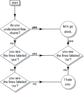
A flow chart about understanding flow charts produced using the diagram package (based on the xkcd comic strip http://xkcd.com/518/).
The diagram package also provides convenience functions for producing simple arrangements of networks of nodes and edges in a single function call, for example the plotmat() function.
Output from the diagram package is produced using traditional graphics; Section 7.5.2 describes some features of grid graphics that can be used to produce similar results based on grid.
Chapter summary
Node-and-edge graphs can be created using the graph package and laid out and rendered using Rgraphviz. The igraph package provides a complete alternative. The diagram package provides tools for producing more regular arrangements of nodes and edges, such as a flow chart, where the layout is determined by the user.
*http://www.graphviz.org/doc/info/attrs.html.