Chapter 14
Maps
Chapter preview
This chapter describes how to draw geographical maps in R. Drawing maps requires specialized extension packages because there are unique file formats for map data and drawing maps involves special transformations that are not provided by the core graphics systems.
From a purely graphical perspective, drawing a map appears to be simply a matter of rendering one or more polygons that represent the borders of one or more countries, states, or regions. For example, it is not immediately obvious whether Figure 14.1 is just a rectangle, or a map of the State of Colorado.

A map of the State of Colorado. This could be mistaken for a simple rectangle because a simple map is just a set of polygonal shapes.
However, a number of issues combine to ensure that producing a map is often not a trivial task.
Map data: The polygons that describe regions on a map can be very detailed and complex, so it is usual to obtain information about map boundaries from external files, which often have a special format. This leads to two problems: locating map data in the first place and then finding functions that can be used to read the map data into R.
Lakes in islands on lakes: One classic example of complexity in a map is the existence of a hole within a geographical region, such as a country that contains a lake. The situation gets worse if the lake contains an island and worse still if the island has its own lake, particularly if the goal is to fill areas of land with a color, but leave areas of water empty. Functions that draw maps must be aware of this problem.
Projections: Locations and regions on a map are often described in terms of geographic coordinates, longitude and latitude, but these are locations and regions on the surface of a three-dimensional sphere whereas map display typically occurs on a two-dimensional page or computer screen. Longitude and latitude are often converted to two-dimensional projected coordinates, which can be drawn in a straightforward manner, but there are many such projections to choose from. Drawing a map requires both knowledge of whether the locations and regions have been projected and, if not, possibly some way of applying a projection to the polygons or other graphical shapes that are to be drawn.
Aspect ratio: The locations of map polygons typically relate to a physical scale, for example, a set of locations on the Earth’s surface. In order to faithfully represent these locations, it is important to control the (ratio of the) physical dimensions of the polygons as they are drawn. Drawing a map requires the ability to control the aspect ratio of the drawing region.
Annotation: A map rarely consists of just the border outline of a geographical region. For example, additional lines may be added to represent other features such as cities, roads, railways, and rivers. More often, the map is just providing a context for displaying the values of one or more variables, such as fill colors to indicate disease incidence within different regions, data symbols to represent the locations of events, or an overlay of weather patterns such as wind speed and direction. Any drawing that consists of multiple layers of annotation like this must ensure that any projection is consistent across all layers. Also, there needs to be some way to reliably match a data value with the appropriate polygon within a map.
The following sections elaborate on these issues and describe some of the packages and functions in R that provide solutions.
This is a very simplified and brief introduction to some of the mapping tools that are available for R. A far more thorough discussion of the ideas, tools, and techniques is provided in the book Applied Spatial Data Analysis with R by Roger Bivand, Edzer Pebesma, and Virgilio Gómez-Rubio.
14.1 Map data
The simplest way to produce a map in R is with the maps package, because maps provides several of its own sets of map information.
14.1.1 The maps package
The maps package provides the function map() for drawing maps. The first argument to this function specifies the name of a “database” that contains the map information. The default is "world", which is a set of low-resolution country boundaries. Other options are: "france", which includes boundaries of the departments of France; "italy", which includes boundaries of the Italian provinces; "state" and "county", which provide state and county borders in the USA; and "nz", which provides the outline of the main islands of New Zealand.
By default, all polygons in a given database are drawn, but the region argument can be used to specify (by name) just a subset of polygons, and the xlim and ylim arguments may also be used to limit the drawing to just a particular range of longitude and latitude.
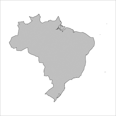
The following code shows a simple example using the default "world" database, but only drawing the polygon corresponding to Brazil (see Figure 14.2).
> library(maps)
> map(regions="Brazil", fill=TRUE, col="gray")
The map() function uses the traditional graphics system to draw the map. The gmaps package can use the maps package map databases, but render the map with grid.
The map produced with the default "world" database is quite coarse and the mapdata package has a higher-resolution map database. For example, the following code produces a more detailed version of Figure 14.2.
> library(mapdata)
> map(database="worldHires", regions="Brazil",
fill=TRUE, col="gray")
However, the map data from both the maps and the mapdata package may not be sufficiently accurate or up-to-date for some purposes. For more modern, accurate, and detailed maps there are more sophisticated sources of map data and more sophisticated packages for working with them.
14.1.2 Shapefiles
A very common format for storing geographical information is the shapefile format. More accurately, such files are called ESRI shapefiles because the format is controlled by the ESRI company that produces GIS software. A shapefile is actually a collection of files; the geographical information is stored in several files with a common name stem and different suffixes (e.g., .shp, .shx, and .dbx).
Shapefiles are available from many places on the internet, including various governmental agencies. Files were obtained from the GSHHS (Global Selfconsistent, Hierarchical, High-resolution Shoreline) database and the Natural Earth Project for the figures in this chapter.*
The maptools package provides several functions to read shapefiles, the most general of which is the readShapeSpatial() function. The following code uses this function to read a shape file that contains state boundaries for Brazil.
> library(maptools)
> brazil <-
readShapeSpatial(system.file("extra", "10m-brazil.shp",
package="RGraphics"))
The maptools package depends on the sp package, which is automatically loaded when maptools is loaded. The sp package provides data structures and functions for working with spatial data in R and this is what gets created by the call to readShapeSpatial(). The variable brazil is a special "Spatial" object that combines the polygons to draw the map, plus extra information about the regions that those polygons represent. The extra information will be used in Section 14.2; for now, the map itself can be drawn with a call to plot(), as shown below, because the sp package defines a method for "Spatial" objects (see Figure 14.3).
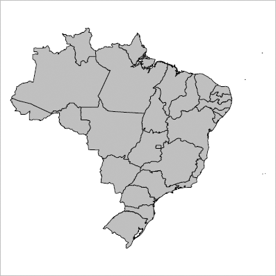
A map of Brazil showing the different states. Made with Natural Earth: Free vector and raster map data @ naturalearthdata.com.
> plot(brazil, col="gray")
The maptools package also provides functions for reading data in other formats, for example, there is the Rgshhs() function for reading map files from the GSHHS database (see Section 14.3). There are also functions for converting map databases from the maps package to "Spatial" objects, for example, map2SpatialPolygons().
14.2 Map annotation
Up to this point, a map has only been considered as a set of polygons representing regions. However, other sorts of shapes are also relevant for drawing maps: lines to represent roads or rivers; and points to represent specific locations of interest such as cities or mountain peaks.
Furthermore, the region boundaries on a map are useful only really as a context for other sorts of data. For example, regions may be filled with different colors to indicate population size and points may be labeled with city names.
This is where the "Spatial" data structures from the sp package become very useful because they contain not only the shapes to draw a map, but also additional information such as place names and region names that are associated with the shapes.
For example, the "Spatial" object brazil contains polygons to draw each of the Brazilian states, plus it contains the name of the region that each state belongs to. The extra information can be accessed just like accessing variables in an R data frame.
> brazil$Regions
[1] Norte Norte Nordeste Norte
[5] Norte Norte Centro Oeste Centro Oeste
[9] Sudeste Centro Oeste Sul Sul
[13] Sul Nordeste Nordeste Nordeste
[17] Nordeste Sudeste Nordeste Sudeste
[21] Nordeste Nordeste Norte Norte
[25] Centro Oeste Sudeste Nordeste
Levels: Centro Oeste Nordeste Norte Sudeste Sul
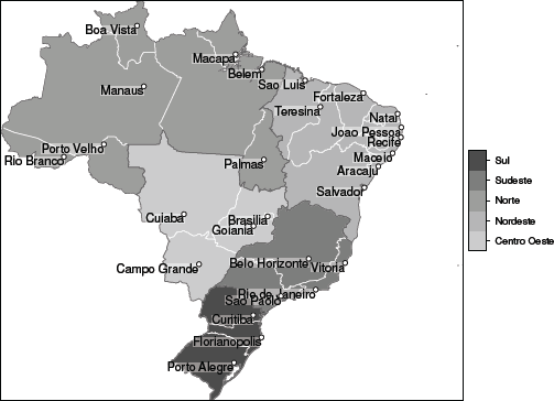
The following code draws a map of Brazil with the states shaded according to region (see Figure 14.4).
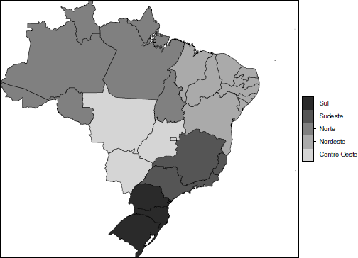
A map of Brazil showing the different state boundaries, with states filled according to which region they come from.
> spplot(brazil, "Regions", col.regions=gray(5:1/6))
This example introduces another function from the sp package for drawing maps, the spplot() function, which provides several points of difference from the plot() method used previously.
The major advantage that has been demonstrated here is that it makes it easy to annotate the fill regions on the map according to the levels of a variable simply by naming the relevant variable. Another difference is that the spplot() function calls lattice functions to draw the map. This means that it is possible to produce multipanel map displays (by specifying more than one variable as the second argument to spplot()) and, because the output is grid based, it is possible to perform detailed customizations.
The next example demonstrates a more complex annotation. In this case, lines, points, and text are added to the original map to indicate the boundaries of regions and the locations and names of the state capitals (see Figure 14.5).
A map of Brazil showing the different state boundaries, with states filled according to which region they come from and state capitals shown.
The data for the region boundaries and the data for the locations and names of the state capitals in this example come from separate shapefiles.
> brazilRegions <-
readShapeSpatial(system.file("extra",
"10m_brazil_regions.shp",
package="RGraphics"))
> brazilCapitals <-
readShapeSpatial(system.file("extra",
"10m_brazil_capitals.shp",
package="RGraphics"))
The following code draws a map with each state colored according to its region similar to before, but with white borders for the regions. The important change is that this time a custom panel function is specified, which adds darker borders around each region via sp.lines(), points for each state capital via sp.points(), and labels for each capital via sp.text(). There are also semitransparent rectangles behind each label to aid visibility. Those are added using low-level grid calls.
> spplot(brazil, "Regions",
col.regions=gray.colors(5, 0.8, 0.3),
col="white",
panel=function(...) {
panel.polygonsplot(...)
sp.lines(brazilRegions, col="gray40")
labels <- brazilCapitals$Name
w <- stringWidth(labels)
h <- stringHeight(labels)
locs <- coordinates(brazilCapitals)
grid.rect(unit(locs[, 1], "native"),
unit(locs[, 2], "native"),
w, h, just=c("right", "top"),
gp=gpar(col=NA, fill=rgb(1, 1, 1, .5)))
sp.text(locs, labels, adj=c(1, 1))
sp.points(brazilCapitals, pch=21,
col="black", fill="white")
})
14.3 Complex polygons
The busy-looking region in the North of the map of Brazil (see, for example, Figure 14.3) represents the mouth of the Amazon river. At the heart of that river mouth lies the island of Marajo, which is large enough to contain its own lakes.
The shape files used in previous figures, from the Natural Earth project, do not have sufficient detail to show these lakes, but the GSHHS database does provide the required resolution. The following code reads in a shapefile that was generated from the GSHHS data.
> marajo <-
readShapeSpatial(system.file("extra", "marajo.shp",
package="RGraphics"))
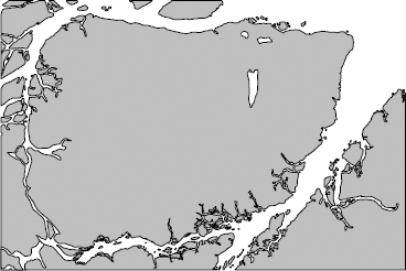
A map of Marajo Island in the mouth of the Amazon River. This is the largest island that is completely surrounded by fresh water in the world. The map data come from GSHHS.
The following code draws Marajo Island and its surrounds. The important features are the three lakes toward the north-east of the island. These have been filled white by specifying the pbg argument.
> plot(marajo, col="gray", pbg="white")
The main point is that the sp functions for drawing maps can detect and handle these situations.
14.4 Map projections
All geographic locations can be specified by a longitude (east-west of greenwich) and latitude (north-south of the equator). However, these are locations on a three-dimensional (approximate) sphere and maps are typically drawn on a two-dimensional page or screen.
A very simple projection of longitude and latitude to a two-dimensional plotting surface involves assigning longitude to the x-axis and latitude to the y-axis, but there are many other possibilities.
In the worst case, no information is known about the map projection. In this situation, the sp functions for drawing maps will set the plot aspect ratio to 1 (a unit in the x-direction is the same physical size as a unit in the y-direction), but that will not always produce a nice result.
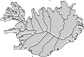
For example, the following code reads in and draws the counties of Iceland without supplying any projection information (see Figure 14.7).
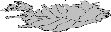
A map of Iceland drawn without specifying any projection information. The result is very distorted because a degree of longitude at northerly climes is a much smaller distance than a degree of latitude.
> iceland <-
readShapeSpatial(system.file("extra", "10m-iceland.shp",
package="RGraphics"))
> plot(iceland, col="gray")
The map data are in geographic coordinates and plotting a country like Iceland by simply mapping longitude and latitude to x and y, with an aspect ratio of 1, creates severe distortion because, at northerly or southerly latitudes, a single degree of longitude spans a much smaller distance than it does at the equator. The following code adds projection information, using the CRS() and proj4string() functions so that R knows that the map is in geographic coordinates. The projection value is a PROJ.4 specification* and this information should be obtained from the supplier of the shapefile or in some cases this will be part of a shapefile in the form of a file with a .prj suffix.
> proj4string(iceland) <- CRS("+proj=longlat +ellps=WGS84")
Now the map can be drawn again (see Figure 14.8). With the projection information specified, the plot() method calculates an aspect ratio for the plot to account for the displacement from the equator and this produces a better result.
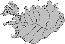
A map of Iceland drawn with an aspect ratio adjustment made for the fact that the map is in geometric coordinates. The result is much less distorted than Figure 14.7.
> plot(iceland, col="gray")
However, the regions for this map of Iceland are still in geographic coordinates. A more sophisticated solution would be to use a proper map projection to produce projected coordinates. This requires loading the package rgdal.
> library(rgdal)
The choice of projection depends on the use for the map because different projections preserve different map features. For example Google Maps uses a Mercator projection because this preserves angles (so that, for example, streets that meet at a cross road are drawn at right angles). The following code projects the map of Iceland using a Mercator projection with the spTransform() function (and then draws the map; see Figure 14.9).
A map of Iceland drawn with a Mercator projection. The result is very similar to the adjusted map of geometric coordinates (which is drawn in gray with white borders in the background).
> icelandMercator <- spTransform(iceland,
CRS("+proj=merc +ellps=GRS80"))
> plot(icelandMercator)
The result is very similar to the previous map, but with this projection the map has known useful properties, rather than just a rough adjustment using the plot aspect ratio.
The following code demonstrates another type of projection. First, projection information is added for the Brazil map used in previous sections.
> proj4string(brazil) <- CRS("+proj=longlat +ellps=WGS84")
Now the map is transformed using an orthographic projection, which shows what Brazil would look like if viewed from orbit at a location above longitude zero and latitude zero (see Figure 14.10). Grid lines have been added to the plot, using the gridlines() function, to help understand the projection.
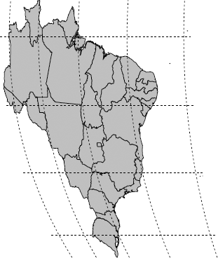
A map of Brazil using an orthographic projection. This is what Brazil would look like from space (hovering above the equator directly south of Greenwich).
> brazilOrtho <- spTransform(brazil, CRS("+proj=ortho"))
> plot(brazilOrtho, col="gray")
14.5 Raster maps
The examples so far have demonstrated vector data (polygonal regions) and point data (city locations). A third main type of information that can be used in a map is raster data, which consists of a regular grid of values (pixels).
Reading and rendering raster data is quite straightforward (see also Chapter 18). The main problem that arises is aligning raster data and vector (or point) data on a map together. The raster package provides support for reading and manipulating raster data, including combining raster and vector data for drawing maps.
> library(raster)
The following code uses the raster() function from the raster package to read in a raster image from the Natural Earth project and sets the projection information using the projection() function. This image provides a grayscale shaded relief of the entire Earth.
> worldRelief <- raster("SR_LR.tif")
> projection(worldRelief) <- CRS("+proj=longlat +ellps=WGS84")
The result is a special "RasterLayer" object and the following code uses the crop() function to reduce that very large image down to just that part of the image that corresponds to the extent of the vector map of Brazil from previous examples. The two objects now correspond to each other and have the same projection, so they can be drawn together.
> brazilRelief <- crop(worldRelief, brazil)
The raster image can be rendered using a "RasterLayer" method for the image() function and then the vector state borders are added using the plot() method for "Spatial" objects, with add=TRUE (see Figure 14.11).

A map of Brazil with a shaded relief background to indicate elevation. Made with Natural Earth. Free vector and raster map data @ naturalearthdata.com.
> image(brazilRelief, col=gray(0:255/255), maxpixels=1e6)
> plot(brazil, add=TRUE)
14.6 Other packages
Several other packages provide further mapping extensions or completely alternative paradigms for mapping in R.
For example, the PBSmapping package provides its own self-contained set of map data files, data structures for working with the map data, and functions for manipulating and rendering the map data. The rworldmap package also contains its own map data plus convenient high-level functions for producing world maps of coarse geographic data sets that contain one value per country.
The RgoogleMaps package provides functions for downloading Google Maps tiles for use as raster map data. Going the other way, there are functions in maptools for writing out map data as KML files for use in Google Earth and Google Maps.
The latticeExtra package provides a mapplot() function for lattice and ggplot2 has the borders() function, plus a few others, to support drawing maps from the maps package.
Chapter summary
Drawing maps requires specialized graphics functions to handle special file formats and rendering details such as map projections and lakes within islands. Simple maps can be drawn using the maps package and its built-in map data. More sophisticated results can be obtained using the maptools package to read in map data, the rgdal package to handle projections, and the sp and raster packages for map data manipulation and map drawing.
*ftp://ftp.soest.hawaii.edu/pwessel/gshhs; http://www.naturalearthdata.com/.