
Chapter 18
The Raspberry Pi in an Analog World
In This Chapter
![]() Discovering what analog means
Discovering what analog means
![]() Creating the Raspberry Ripple
Creating the Raspberry Ripple
![]() Making a Steve Reich machine
Making a Steve Reich machine
![]() Building a light-controlled instrument
Building a light-controlled instrument
![]() Making a thermometer
Making a thermometer
In the previous two chapters, we show how the Raspberry Pi could sense logic levels on the GPIO pins when they were configured to be inputs. We also show how you could switch LEDs on and off when GPIO pins were configured to be outputs. We also show how, by using a transistor, you can use the Pi to control much larger currents than you can get directly from the GPIO pins.
In this chapter, we show you how to use the GPIO to talk to other integrated circuits. There are many ways to do this, called protocols. This chapter concentrates on one called the I2C protocol. Many integrated circuits use this protocol to allow you to do many things. However, one very different sort of thing is how to input and output, not in the strict on/off way of the digital world you have seen so far, but in an analog or proportional way.
In this chapter, we show you how to make the Raspberry Ripple, a board to allow you to input and output analog signals. Then we explore some of the interesting things that you can do in this new analog world.
Exploring the Difference: Analog versus Digital
With a digital signal, everything is either on or off, no half measures. Indeed, many things work in this manner; for example, your radio is either on or off. It makes no sense for it to be anything else. However, this is not true of everything. For example, a light can be half on or dimmed. A volume control can be full on, full off, or somewhere in between. These are proportional controls.
Taking small steps
So how does a computer handle a proportional control? In a program, variables can take on any value you assign them. You can do the same with a voltage. However, the voltage is not continuously variable, but split up into small steps, or quantized. The number of small steps used is given by the resolution of the circuit. By combining several on/off signals, with each one contributing an unequal small voltage, you can produce very close to whatever voltage you want. The circuit to do this is called a digital-to-analog (D/A) converter, and there are several different designs. Figure 18-1 shows one such method using four digital outputs, or as we say, four bits. Each switch is a digital output from the computer and can send current through a resistor or not, depending on whether the switch is open or closed. The important thing is the relative resistor values, not the absolute values.
The resistor R is any value and 2R is twice that value, 4R four times, and 8R eight times. The voltage that is switched is called a reference voltage or Vref and is in effect the maximum voltage that will be output. The current from each of these switched resistors is fed into a current summing circuit. The output of the summing circuit is driven through a resistor with a value of R, shown in Figure 18-1 as Rs.
To see how this works, suppose only switch 3 is made. Current I3 flows into the current summing circuit, and, as no more switches are made, that is the current that flows out of the current summing circuit. This flows through Rs and thus develops a voltage across the summing resistor. As the resistor on Sw3 has a value of R and the summing resistor has a value of R, the voltage developed across the summing resistor is equal to half the reference voltage. If only switch 2 is made, the output voltage is a quarter of Vref; similarly, switch 1 produces an eighth and switch 0 a sixteenth. When more than one switch is made, the current from each switch is added together and produces an output voltage, Vout, which is the sum of these fractional voltages of Vref.

Figure 18-1: Four switches and resistors make a digital-to-analog converter.
With four switches, you can have a number of combinations of switches made and unmade. The total number of combinations is given by two (the number of states) raised to the power of four (the number of switches). So we can have 16 different combinations and so 16 different voltages out of Vout. Table 18-1 shows each one of these. Note that the voltages are not “nice” round values and that the maximum voltage is just short of the reference voltage, or Vref. In fact, it is short by one increment; that is, by one sixteenth of the reference voltage.


As there are four switches, we say that this D/A has a resolution of four bits. If you replace the open and closed in the switches columns with logic 0 and 1s, the whole thing starts to look like a binary number, which is exactly how a computer stores an integer variable. Four bits is rather coarse, and a typical D/A converter can normally have anything from 8 to 16 bits, with even 24 bits being possible. With a 16-bit converter and a 5V reference voltage, each voltage step will be
5V/(216) = 5/65536 = 0.00007629395 V or 76.29395 uV
Those still aren’t nice round numbers, but it’s very fine control indeed. In fact, this is a much smaller step that any interference or noise likely to be in most digital circuits. We cover this interference in Chapter 15. So the step size is small compared to circuit noise. For all intents and purposes, the voltage output can be thought of as continuously variable.
Reading small steps
You can see how, by combining lots of outputs, you can make a voltage that is adjustable in small steps. But what if you want to read how big a voltage is — that is, perform the opposite task of an analog-to-digital conversion (A/D)? You have to have a D/A along with a circuit known as a comparator. A comparator is simply an amplifier with a very high gain. It has two inputs marked: + (plus sign) and − (minus sign). Its output is high if the + input has a higher voltage on it than the − input. If the − input is higher, however, the output is low. So a comparator simply produces a signal that tells you which input is higher. Team that up with a D/A and you have an A/D, as shown in Figure 18-2.

Figure 18-2: A block diagram of an analog-to-digital converter.
This is a block diagram, which means it only shows how a thing works, not the wiring you need to make it work. A new symbol here is the thick line with a slash across it and the number eight above. This means that there are really eight wires here, each one going into the D/A. Into these go a number, denoted by a combination of high and low lines, which is a guess as to what our unknown voltage will be. If the guess is too high, the comparator output is high; if the guess is too low, the output is low. To find the exact value of our unknown voltage, you must find a number that results in a low output of the comparator, yet with only an addition of one to the number results in that output being high.
This means that in order to get the A/D to function it has to be driven; that is, something must implement an algorithm of guesses and responses to the guess. This can be done with dedicated logic circuits or it can be driven from a computer. The simplest algorithm is called a single ramp. The guess is incremented by one repeatedly until it reaches the value of the unknown voltage. This is simple but not very efficient. A much more efficient way is to use successive approximation.
Suppose you are asked to guess a number between 0 and 256 and the only information you could get is whether your guess is too high or too low. The best strategy is to guess at half the range and keep on halving. So your first guess should be 128. If that’s too low, your next guess should be between 128 and 256, so halve that and guess 192. It that’s too high, you know the number is between 128 and 192, so halve the difference and guess 160. Keep repeating that, and in only eight guesses, you will have honed in on the correct number.
Investigating Converter Chips
Special chips have all the circuitry and can do all of these processes for you. Your computer can connect to these chips in a wide variety of ways. One of the simplest ways is called a parallel connection, where each signal in the circuit has a separate GPIO pin allocated to it. It is the fastest way, but it uses a lot of GPIO pins. A more efficient way is to send data one bit at a time over a single wire along with another wire that changes to signify a change in data. This other wire is called a clock signal. One of the more popular implementations of this sort of communications is to a protocol called I2C.
This protocol has been around for a long time. It was first produced in 1982 by Philips to allow its ICs to communicate. The initials stand for Inter-Integrated Circuit communication. This is sometimes abbreviated to IIC or I2C, otherwise known as twin wire. It’s pronounced “eye squared cee” and should be written as I2C, but not all computer systems or languages have the facility for superscript capability, so it remains I2C in most places.
The idea is that communication takes place over two wires: One carries the data and the other the clock. As there is only one line for the data, and that can only be high or low, transmitting numbers or bytes (a collection of 8 logic levels defining a number) happens serially; that is, one bit at a time. The rising edge of the clock line tells the receiver when to sample the data signal, and each message to and from a device consists of one or more bytes.
In its simplest form, there is one master device, which in our case is the Raspberry Pi, and up to 128 different slave devices. In practice, there are very rarely this many, and it is normal just to have one or two. Each slave device has to have its own unique address, and this is, in the main, built into the chip you are using. The first thing in any message from the master is the address of the slave it wants to communicate with. If a slave sees something that is not its own address, it ignores the message.
Building the Raspberry Ripple
What you are going to make next is the Raspberry Ripple, an analog input/output board. In electronics, the word ripple is used to denote small, often rapid, changes in a voltage. This board is going to look at changing voltages, hence the name. After you’ve made it, you can make a whole range of projects with analog signals. We show you some examples at the end of the chapter.
Here are the parts you’ll need to build the Raspberry Ripple:
- 1 2.8"×1.7" copper strip prototype board.
- 1 16-way DIL IC socket.
- 1 PCF8591P 8-bit A/D and D/A converter.
- 1 2N2222 NPN transistor.
- 1 1N4001 diode (or any other diode).
- 2 47uF capacitor 6V8 or greater working voltage.
- 1 1K wire-ended resistors.
- 5 3-way PCB mounting terminal block with screw connectors.
- Note the Phoenix contact–PT1,5/6-5.0-V–terminal block, PCB, screw, 5.0mm, 6-way can be split in half by sliding the components apart.
- 2' 24 SWG (or similar) tinned copper wire.
Note: A 10K potentiometer might be required for testing.
The chip at the heart of the Ripple
At the heart of the Raspberry Ripple is the PCF8591 chip, a venerable design that has stood the test of time. It is widely available, but the price can vary dramatically depending on where you buy it. It contains a four-input, 8-bit A/D converter and a single output 8-bit D/A converter. In fact, it only has one A/D converter, and the four inputs are achieved by electronically switching from one of the four inputs into the A/D converter. It has three external address lines, which means that part of the address of this chip can be determined by how these lines are wired up. This means that up to eight of these chips can coexist on the I2C bus and all have their own unique address. The other 4 bits of the address are fixed. When you know what bits need to be set, you can find the address by adding up the value of each bit with a one in it, as shown in Figure 18-3.

Figure 18-3: Determining the address of a PCF8591.
Putting the chip into a circuit
The schematic of the Raspberry Ripple is shown in Figure 18-4. There isn’t much to it apart from the chip. However, one component we have not met before is the capacitor. There are two here, C1 and C2. Their job is to smooth out any variations, or noise, on the power supply to the chip and the reference voltage. The reference voltage needs to be stable because if it changes, the voltage reading changes, even if there is no real change in the input voltage. Adding a resistor and having another capacitor on the voltage reference pin gives a more stable reference than just connecting it to the supply. The capacitors have a working voltage associated with them. As long as it’s more than 5V, it doesn’t matter what it is. However, the higher the voltage, the bigger the capacitor will be.

Figure 18-4: The schematic of the Raspberry Ripple.
The diode D1 is there to drop the supply voltage by a tad. Although a diode is used to restrict current flow in one direction, when current is flowing through, it drops a constant voltage across it of about 0.7V independent of the current flow. Strictly speaking, you need this because the Raspberry Pi can only deliver a 3V3 signal, and the lowest signal the data sheet says can be seen by this chip as a logic one is 0.7 of the supply voltage. If the supply voltage is 5V, the signal must be 3V5 to be recognized. In practice, we’ve found it works quite happily without the diode, but going against the information in the data sheet is a very bad idea because you have no guarantees of anything.
We have wired address line 1 to the supply to make it a logic one, and the other two address lines to ground or logic zero, to give the address 74. You can have up to eight of these circuits running at the same time. You just have to ensure that each circuit has a different combination of logic levels wired to these address lines.
The four analog inputs are wired to their own three-way screw terminal block with both a ground and a supply voltage on them. We used Phoenix contact–PT1,5/6-5.0-V–terminal block, PCB, screw, 5.0mm, six-way. They are in fact two three-way blocks and it is easy to just slide them apart. It is actually cheaper to buy a six-way block and split it than it is to buy three-way blocks. These screw terminal blocks have a blank area next to the contact that is ideal for putting a label on. Using a screw block makes wiring up the later projects to this a lot easier. The analog output of this chip is fed directly to a screw terminal and through a transistor to act as a current buffer if you need to get more drive from the output.
Wiring it up
Figure 18-5 shows the layout of the Raspberry Ripple on strip board. Note the hidden detail showing where the tracks are cut between the adjacent pins of the IC as well as in four other places. Figure 18-6 shows a photograph of the same thing. The capacitors must be placed the right way round. The positive end is marked by a depression in the can and the negative end by a black line in the type (the marking might be different on other types). The diode has a line marking the cathode or pointy end of the symbol. All the diodes we’ve seen are marked like this. Finally, the chip has to be fitted the right way round as well. It has a small circular indent marking the top.
Note the link next to the +ve connection on the A1 connection block. Here two wires go into the same hole, denoted by the gray hole. Put both wires through before soldering them up. We also used an IC socket for the chip so it could be replaced in case of accidents. The board is wired up to GPIO pins 2 and 3 (or 0 and 1 if you have an issue 1 board). These two different GPIO signals are physically on the same pins for the two board issues. Unlike the other projects in this book, you have no choice in pin assignment because we are going to use these pins’ special hidden powers to talk to the chip.
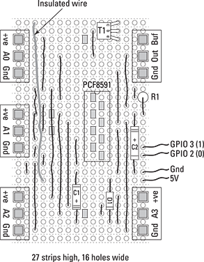
Figure 18-5: The wiring layout of the Raspberry Ripple.
Installing the drivers
Before you can use the Raspberry Ripple board, you have to install an I2C driver to allow the GPIO pins to become a specialist I2C bus driver. This means that the Raspberry Pi’s hardware will handle the transfer of data along these two wires. A few drivers are available, but the SMBus driver is by far the easiest to install and the commands are quite easy to use. In fact, many distributions already have it installed as standard, but by default it is disabled. To enable it, you have to change two files. Type the following into the command line:
sudo nano /etc/modprobe.d/raspi-blacklist.conf
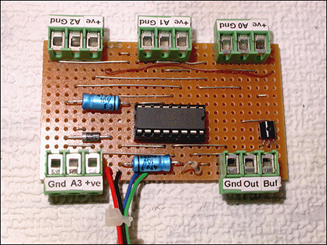
Figure 18-6: A photograph of the Raspberry Ripple.
Add a # at the start of the line blacklist i2c-bcm2708 and then press Ctrl+X. Press Y to save and exit. Next, you need to edit the modules file, so type
sudo nano /etc/modules
Add a new line to this file that says i2c-dev. Again, press Ctrl+X and then press Y to save and exit. Install a handy little utility for checking what is on the I2C bus by typing two lines:
sudo apt-get update
sudo apt-get install i2c-tools
Finally, you need to tell the system you can use it. Assuming you still have the default user name of pi, type
sudo adduser pi i2c
Then reboot the machine with
sudo shutdown -h now
Remove the power, plug in the Raspberry Ripple board, and power it up again. After you have logged in, type
sudo i2cdetect -y 0
You should see a table with all blank entries except one saying 4a, which is the address, in hexadecimal, of the Raspberry Ripple board. Remember, this is the same as the decimal value of 74 you calculated earlier in the chapter. If you do not see this address, check the wiring again for any errors. One big advantage of installing the drivers in this way is that you can now run your Python programs direct from the IDE. You don’t need to run them with root privileges with a sudo prefix.
Using the Raspberry Ripple
Now we are ready use the Raspberry Ripple board. The first thing you need to do is to learn how to talk to the board and test it out. The PCF8591P has one control register: This is a single 8-bit (one byte) memory location in the chip that controls how it operates. So when you talk to the chip, you first send it an address, then the control byte, and then the data you want to send. The control byte is shown in Figure 18-7 and is a simplified version of that shown in the data sheet. We encourage you to download the data sheet and read it. It contains far more than you need to know and like any data sheet, it can be a bit intimidating when you first see it. However, it will describe the alternative input configuration modes that we’re not using here. You will just be using the straightforward four channels of analog input in this book.

Figure 18-7: The PCF8591P control register.
You will see that the control byte has one bit, bit 6, that controls whether the analog output is enabled. It also has two bits that select what analog channel to read, and there is also a bit that enables the auto-incrementing of the channel select. This is useful because it means that you can look at all four input channels just by doing four successive reads. You don’t need to set up the channel first.
Just a word of caution — when you read an analog channel, you do two things. You get back the last reading and you trigger the next one. Sometimes this is not a problem, but at other times, you have to bear in mind that’s what is happening.
Testing the analog inputs
If an input channel is not being used, you should wire it to ground; otherwise, you get wildly fluctuating results from it. Therefore you need to put a wire between the A1, A2, and A3 input and the respective ground for this first test. Next you need to wire a variable voltage source to A0. The simplest and best way of doing this is to use a new component: a potentiometer or pot, sometimes also called a variable resistor. Basically, it’s a knob. It has three terminals and is shown in Figure 18-8. They come in a variety of values. You’re better off using a 10K one for this experiment, but any value between 1K and 47K will do. If you wire the middle terminal or wiper to A0, wire the bottom end connections to ground and the top end to +ve. Now you’re ready to run the program in Listing 18-1. Note that the only thing that will happen if you swap the top end and the bottom end around is that it will produce the maximum voltage when it is turned fully anti-clockwise (counterclockwise).

Figure 18-8: A potentiometer.
Listing 18-1: Analog Input A0 Reading
# Read a value from analog input 0
# in A/D in the PCF8591P @ address 74
from smbus import SMBus
# comment out the one that does not apply to your board
#bus = SMBus(0) # for revision 1 boards
bus = SMBus(1) # for revision 2 or 3 boards
address = 74
Vref = 4.3
convert = Vref / 256
print("Read the A/D channel 0")
print("print reading when it changes")
print("Ctrl C to stop")
bus.write_byte(address, 0) # set control register to read channel 0
last_reading =-1
while True: # do forever
reading = bus.read_byte(address) # read A/D 0
if(abs(last_reading - reading) > 1): # only print on a change
print"A/D reading",reading,"meaning",round(convert * reading,2),"V"
last_reading = reading
This simply reads the voltage value on analog input channel 0 and prints it out if it has changed. The program prints out two values: The first is the raw A/D converter reading and the second is what this means in terms of volts. The values the program prints is restricted to two decimal places because 8 bits resolution does not justify any more significant digits. In calculating the voltage from the reading, the variable Vref is used to hold the reference voltage. This is right only if your Raspberry Pi is running off exactly 5V, something that is a bit unusual. To make this voltage value more accurate, use a volt meter and measure the voltage across C2; that is, place each of the two volt meter leads to each end of the capacitor.
If you get a negative reading, swap them. Take the value you measure and put it in as the value for Vref in the program. This applies to all the listings with a Vref variable. However, many programs you write using an A/D are not interested in the actual voltage but just use the raw reading. You can modify the listing to read any of the input channels by simply changing the value in the bus.write_byte instruction to change the control register so it selects another channel.
Testing the analog output
To check out the analog output, you need an LED and resistor wired up as shown in Figure 18-9. The wire to A1 is for the next experiment, so you can leave it out for now. Enter and run the program in Listing 18-2.

Figure 18-9: A test LED circuit.
Listing 18-2: D/A Output Ramp
# Output a count to the D/A in the PCF8591P @ address 74
from smbus import SMBus
from time import sleep
# comment out the one that does not apply to your board
# bus = SMBus(0) # for revision 1 boards
bus = SMBus(1) # for revision 2 & 3 boards
address = 74
control = 1<<6 # enable analog output
print("Output a ramp on the D/A")
print("Ctrl C to stop")
while True:
for a in range(0,256):
bus.write_byte_data(address, control, a) # output to D/A
sleep(0.01)
You see the LED blink on and off, but on closer inspection, you see it rapidly fade up and then blink out. What is happening here is that the voltage output is gradually increasing as the for loop outputs successively bigger voltages. At some point, the LED comes on and gets brighter as more current flows through it. Note how it appears to stay the same brightness for a time even though the current through it is rising. This is due to the logarithmic light response of the human eye.
Making a Curve Tracer
You are going to make a curve tracer; that is, a device that outputs a varying voltage, applies it to a simple circuit, and reads back a measurement. When using the analog output, the analog input A0 is not functional and must be left unconnected. The analog input A1 has a high-value pull-down resistor to stabilize the readings when no voltage is applied. This resistor doesn’t affect the measurements. In Listing 18-3, the voltage across the LED is measured by analog channel A1 and printed out along with the analog output voltage. Look at how the voltage “sticks” at close to the LED’s turn-on voltage. When the LED is on, the voltage across it does not rise by much despite the voltage applied to the whole thing increasing. This sticking voltage depends on the LED’s color and type.
Listing 18-3: LED Curve Tracer
# LED_trace1 - Buf --resistor -- A1 -- LED -- Gnd
# Print the voltage across an LED a voltage applied to LED and resistor
from smbus import SMBus
from time import sleep
# comment out the one that does not apply to your board
bus = SMBus(0) # for revision 1 boards
# bus = SMBus(1) # for revision 2 boards
address = 74
control = 1<<6 | 1 # enable analogue output and set to read A1
Vref = 4.44
convert = Vref / 256
print("Output a ramp on the D/A")
print("Ctrl C to stop")
while(True): # do forever
for v in range(28,256): # start close to 0.7V
bus.write_byte_data(address, control, v) # trigger last value to D/A
bus.write_byte_data(address, control, v) # trigger this value to D/A
reading = bus.read_byte(address) # read to kick off conversion
reading = bus.read_byte(address) # read value
Vbuf = (convert * v) - 0.7 # compensate for 0.7V lost ![]()
in the buffered output
if Vbuf < 0:
Vbuf = 0
Vin = convert * reading
if Vin > Vbuf:
Vbuf = Vin
Vout = convert * v # raw output voltage
print "Out",round(Vout,2),"V Buffered",round(Vbuf,2) , ![]()
"V --> Measured input 1 ", round(Vin,2),"V"
sleep(0.01)
The circuit is being driven from the buffered output of the Raspberry Ripple. The normal output of the Raspberry Ripple goes through a transistor in a configuration known as an emitter follower. This transistor allows the Ripple to drive much more current into a circuit than the PCF8591P alone; however, it does slightly complicate things. The voltage on the emitter follows the voltage on the base, with an offset of 0.7V. For example, if you output 2.7V from the D/A, you get 2V on the buffered output. This means that if you are ramping up the voltage to a circuit, there will be nothing out of the buffer until there is 0.7V going out.
To compensate for this, an offset is subtracted from the output value in the program. However, if the output value is below 0.7V, subtracting this offset results in a negative output value, which of course is absurd. Therefore, the program zeros the calculated buffered output if it’s negative.
You can get the list of reading produced by this program plotted out as a graph of applied voltage against voltage across the LED. See if you can write a program to do this. If not, there is one on the website for this book called LEDtrace2. (See this book’s Introduction for more on how to access the website.) A more normal sort of curve for an LED is the voltage against current. You can plot this by just taking the difference between the voltage across the LED and the voltage being output, giving you, in effect, the voltage across the LED’s resistor. This voltage is directly proportional to the current and can be used as a current reading.
In fact, because you have three working analog channels, you can measure three curves at once. Figure 18-10 shows the circuit to plot the curve from a variable resistor and two different colors of LED, red and blue. Note the top end of the pot is not connected to anything. All three are plotted at once as shown in Figure 18-11. Again, you can find the program to do this on the website for this book. It’s called LEDtrace4. The resistor is a simple straight line whose slope is determined by the resistor value. Because there is a pot acting as a resistor in the A1 input, altering the pot’s value changes the slope of the curve. Any coarseness in the plotted graph is simply the inevitable noise or dither on the least significant bit you get with any A/D conversion.

Figure 18-10: Wiring up two LEDs and a pot.

Figure 18-11: The results of plotting the curves for two LEDs and a pot.
Making a Pot-a-Sketch
You are now well on your way to exploring what the Raspberry Ripple board can do for you. Next up you can make “pot-a-sketch,” or a pot box drawing tool. This is simply four potentiometers in a box. Figure 18-12 shows the schematic and Figure 18-13 shows a photograph of the finished product. We used a small plastic box and push-on knobs with red, green, blue, and yellow push-on tops. For this program, you have one pot for the X movement and one for the Y movement, with the other two defining the color in terms of hue and saturation. The Delete key or spacebar is used to wipe the screen clean. Figure 18-14 shows a screen dump of it in action. Fire up the program pot-a-sketch.py and twiddle the knobs to make your drawing. Again, the code to drive this is on the website. (See this book’s Introduction for more on how to access the website.)

Figure 18-12: The schematic of the pot box.
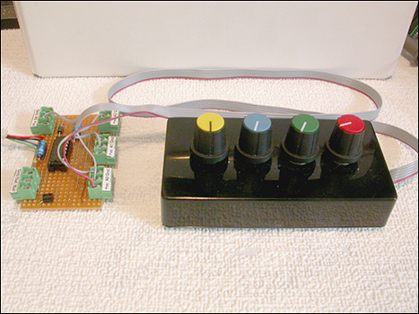
Figure 18-13: The pot box wired to the Raspberry Ripple.
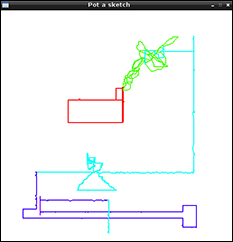
Figure 18-14: A scribble produced by Pot-a-Sketch.
Making Real Meters
Do you want to have the readings from the pots displayed like a real meter? Figure 18-15 shows a program that does this. Basically all that is happening is that the analog reading is used to set the angle of a line. This is plotted over the top of an image of a meter we created in Photoshop on a desktop computer. You can find the program to do this called PotMeter4.py on the website that accompanies this book and use it as a basic analog input check or incorporate it into you own program.
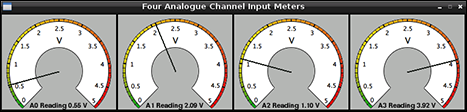
Figure 18-15: Displaying real meters.
Making a Steve Reich Machine
Without changing the hardware, you can use these four pots to control your very own Steve Reich machine. Steve Reich is a well-known modern composer whose signature sound is one of slow development of a repetitive motif, often played on one or many marimbas. This program has eight sound samples of a scale played on a marimba, and it plays them back in a sequence of eight notes. After a number of repetitions, the sequence is mutated by replacing some of the original notes with new ones. Using the pot box, you can control the speed of the notes, the number of repeats before mutation occurs, and the number of notes that are changed in a mutation. You can also control whether the notes are playing. An interesting effect can be achieved by disconnecting the A0 input channel — controlling the speed. This then reads wildly fluctuating values and gives the output a bit of a random rhythm. The program is called Pot_Reich.py and can be found on the website that accompanies this book.
However, the magic of this program literally comes to light when you replace the pots with light-dependent resistors (LDRs). As the name implies, these devices change their resistance depending on the strength of light falling upon them. Although the Raspberry Ripple can’t measure resistance directly, it’s easy to make the LDR produce a voltage by simply putting it in series with a resistor, putting a voltage across it, and measuring the voltage across the LDR with the Raspberry Ripple.
Figure 18-16 shows how this is wired up for one channel. You can replace as many pots as you like with your hand control. We used a cheap LED reading light to shine on the LDRs and then moved our hands over them to change the readings. The code needs a bit of a tweak to adjust for the reduction in range the light controls have compared to the pots. The 27K resistor also affects the range. You might have to change the value of the resistor a little if you get another type of LDR. A program with these code tweaks called Light_Reich.py is on the website that accompanies this book.
Another program on the website that accompanies this book is called Light_Play.py uses four LDR sensors to trigger the notes themselves, like a four-note instrument played by waving your hands over the sensors. You can see a video of this in action at https://vimeo.com/62776651.

Figure 18-16: Wiring up a light-dependent resistor.
Taking the Temperature
Finally, here is a quick way to measure temperature. The LM335 is a cheap temperature sensor. In its cheapest form, it’s in a plastic package and looks just like a transistor. However, with the simple addition of a 1K resistor, it can produce a voltage across it that is proportional to the absolute temperature in degrees Kelvin. The connection to the Raspberry Ripple is shown in Figure 18-17. The resistor goes from the +ve to the analog input, along with the center pin of the LM335, and the right pin goes into the ground. The LM335 can be clamped to a surface to measure its temperature, or if you seal the wires with silicone rubber, you can measure the temperature of liquids.
Note that the left pin is not connected to anything. For each degree Kelvin increase in temperature, the output increases by 10mV or 0.01 of a volt. Because the Raspberry Ripple can detect a change of about 15mV, we can use this chip to measure to the nearest two degrees. For a more accurate reading with this sensor, you need to use an A/D converter that has more resolution; that is, more bits. To calibrate this temperature measuring system, you need to take the difference between the reading and the real temperature. A simple addition or subtraction of a constant is all that you need to do. The code, called Read_temp.py, is on this book’s website. For more on accessing the website, see the Introduction to this book.
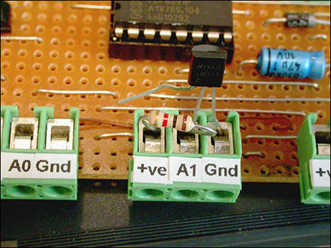
Figure 18-17: Attaching an LM335 temperature sensor.