Achieving Quality in Customer-Configurable Products
Martin Große-Rhode; Robert Hilbrich; Stefan Mann; Stephan Weißleder Fraunhofer Institute for Open Communication Systems, Berlin, Germany
Abstract
Customers of products that include or are determined by software today expect the product to be individually configurable. At the same time high quality and short delivery times are expected. As a consequence, the producer of the software must be able to develop systems that can be easily configured according to the customer’s needs in such a way that each individually configured system satisfies all quality requirements. Especially in the case of high numbers of possible configurations, it is obvious that it is not feasible to construct all system configurations and check the properties of each of them. Rather, there must be means to assure quality generically, meaning once and for all configurations at the same time. This chapter considers software product line engineering as the base technology for how to construct configurable systems and add generic quality assurance means to this process. The mechanism can be understood as a general pattern explaining how to carry over quality assurance techniques to configurable systems. This is done for two concrete techniques in the chapter: model-based testing as a technique for the assurance of functional quality and model-based deployment as a technique for the assurance of real-time properties such as responsiveness, availability, and reliability. The techniques are demonstrated using the example of a configurable flight management system as found in modern airplanes.
Introduction
Beyond achieving pure functionality, system quality is one of the most important aspects of systems engineering. It contributes essentially to the satisfaction of customer needs, the reduction of after-sales costs, and the certification of products. Besides high quality, customers now also want products that are tailored to their needs. For this reason, configurability of products becomes more and more important, and manufacturers strive to adapt their engineering processes correspondingly. Product line engineering (Clements and Northrop, 2002) is an established approach to the development of configurable systems and gradually replaces single product engineering. The focus of this chapter is therefore on quality assurance in product line engineering with the aim to support the systematic development of high-quality configurable systems.
The series of international standards named systems and software quality requirements and evaluation (ISO/IEC, 2014) distinguishes management, modeling, measurement, requirements analysis, and evaluation as the essential activity domains to achieve system quality. One of the main insights throughout all these domains is that quality has to be addressed throughout the whole process; it cannot be added to the finished product at the end. Corresponding to this, we introduce a framework explaining how quality assurance can be established in product line engineering. We instantiate and demonstrate this framework with two quality assurance techniques that are applied at different stages of the engineering process: model-based testing (MBT) as a technique to measure both the functional suitability and the testability of the engineered systems and model-based deployment as a means to establish system reliability, availability, responsiveness, and other qualities that depend on its real-time behavior.
In this sense we understand configurability as orthogonal to other qualities such as those just mentioned. Correspondingly, the purpose of the framework is to lift a quality assurance technique—such as MBT and model-based deployment—from the level of single products to the level of product lines. This is equivalent to saying that the framework helps to achieve customer configurability as additional quality for systems whose further qualities are achieved by other techniques in that it extends these techniques to product lines instead of single products.
Product lines differ in the number of product variants and the number of products per product variant, depending on the application domain and the industrial sector. We sketch two examples in the following.
To give an initial understanding of product lines and configurability, we first consider the development of software for vehicles. There are millions of product variants, but a comparatively small number of products per product variant. Customers expect that they are able to configure their desired car, which means that they can select the equipment and functionality of the car according to their needs and desires. Today, software is embedded in almost every part of a vehicle. Consequently, the functionality as well as the equipment of the vehicle define requirements for the vehicle software. Thus, the car manufacturer has to build configurability into the software system that allows the production and delivery of the individual system requested by the customer in short time. This induces the following constraints. On the one hand, the expected time duration between the receipt of the customer’s order and the vehicle’s delivery is too short to allow creative or extensive development and quality assurance steps. As a consequence, the production process of an individual car, including its software, must be precisely defined and the assembly must be a matter of routine. On the other hand, the number of possible car configurations is too high to allow building and testing all variants before the market introduction: Vehicles today have more than a million variants and many of them have an impact on the software system configuration. Configurability thus means to build one generic system from which all possible individual configurations can be derived in such a way that the car manufacturer may trust in the quality of each individual configuration with respect to aspects such as safety, dependability, availability, usability, and security, for example.
As a further example, let us consider the development of software for airplanes. This domain is characterized by a small volume production. Nevertheless, configurability is required. For instance, airlines as the customers of airplane manufacturers often want to design the cabin on their own or integrate third-party systems into the airplane. Furthermore, every single end product must be approved for the target market and be certified by the authorities of the customer’s states. However, the manufacturer of the airplane is responsible for the approval. In this sense, the manufacturer needs to develop a high-quality system that is configurable and compatible with the individual contributions of customers and at the same time satisfies the requirements on the integrated final system. The situation is similar for subsystem suppliers in any other domain: They typically produce solutions for different manufacturers and, therefore, have a strong interest in building systems that can be adapted to the different customer’s requirements while satisfying their quality requirements.
Outline of the chapter
Having given a rough introduction to configurable systems and an explanation of why it is important to stress the focus on quality of those systems, we detail this in Section 9.2. Furthermore, we provide a framework describing how techniques for quality assurance of configurable systems can be implemented. For this purpose, we first introduce the means to integrate the needed flexibility into a systems engineering process (Section 9.2.1). Then, in Section 9.2.2, we describe how a quality assurance concept in this context can be set up.
Afterwards we show how to apply this concept to two different quality assurance techniques: MBT is a common technique used to attain confidence in a correctly implemented functionality. We discuss in Section 9.3 how to apply MBT to configurable systems. Model-based software deployment is another quality assurance technique that provides a means to construct correct and good deployments according to predefined safety and resource constraints. By this, performance, efficiency, and reliability quality aspects can be ensured. How model-based deployment can be applied to configurable systems is discussed in Section 9.4.
We substantiate the explanations with example models that describe the properties of a flight management system (FMS), which is introduced in Section 9.1. To conclude, we give an overview of related work in Section 9.5 and summarize this chapter in Section 9.6.
9.1 The Flight Management System Example
A FMS is a central and important part in the aviation electronic systems (avionics) of modern airplanes. It supports a variety of in-flight tasks by providing the following set of information functions: navigation, flight planning, trajectory prediction, performance computations, and in-flight guidance. In order to implement these functions, an FMS has to interface with a variety of other avionics systems. Due to the importance of an FMS for the safe operation of an airplane, most of its functions have to be highly reliable and fault-tolerant. Although the specific implementations of an FMS may vary, it generally consists of a computer unit and a control display unit. The computer unit provides the resources for all computationally intensive calculations and establishes the interfaces to the other avionic systems. The control display unit is the primary interface for the pilots. It is used to enter data and to display the information provided by the FMS. The computer unit for small FMSs with a reduced set of functionalities can be realized as a non-standard stand-alone unit. However, for larger FMSs, the computer unit often requires the use of powerful and fault-tolerant processing resources, such as the Integrated Modular Avionics (IMA) (Morgan, 1991; Watkins and Walter, 2007) platform in modern airplanes. We use the development of a configurable FMS as running example in this chapter.
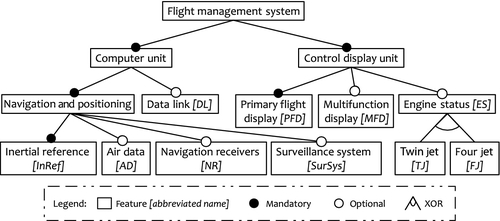
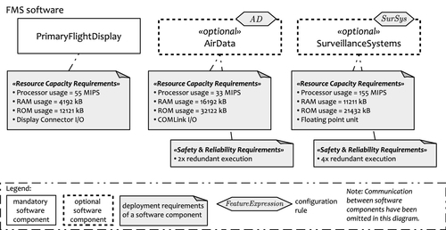
The customer-visible set of features of the envisioned product line is depicted in Figure 9.1. Each feature corresponds to a system-level function of the FMS. In Section 9.3 we focus on the application level functionality of the FMS and analyze how test cases can be derived. For that purpose the system’s functionality is modeled as a configurable state chart in Figure 9.3. In Section 9.4 we discuss deployments issues. Figure 9.7 illustrates the application level of FMS by showing some of the FMS software components and their hardware requirements. In Figure 9.8 the configurable hardware architecture of the FMS is illustrated.
9.2 Theoretical Framework
In this section we present the preliminaries and the theoretical framework of our approach. As indicated above, in order to achieve system quality, it must be addressed throughout the whole engineering process. Given that we focus on such complex safety-critical systems as the ones mentioned in section “Introduction”, we assume that a defined software development process is given and that models are used, for instance, to capture and analyze the requirements, to design the abstract functionality of the system, or to design the software architecture. In the case of embedded systems, the development of the underlying computing platform can also be supported by models that define the topology of the system, the communication means, or the capacities of the nodes in a network. Accordingly, we discuss in this section how models can be extended to express configurability from different viewpoints and how the quality of a configurable system (under development) that is represented by such models can be assured.
9.2.1 Configurable models
Before we define how to express configurability in a model, we first have a closer look at which kinds of models we consider and where the distinction of different models or views comes from.
9.2.1.1 System views
In this chapter, for the sake of simplicity, we consider only three views that are to be described by models.
1. The application level view in which the functionality of the system from the point of view of the user is considered.
2. The resource level view in which the computing platform (nodes, networks, hardware resources) are described.
3. And the deployment view that describes how the resources are used to realize the application functions. These views correspond to those suggested by Kruchten (1995), which we discuss below. To simplify matters, we do not explicitly distinguish between the logical and development views here, but we highlight the deployment view in Kruchten’s physical view because of our emphasis on embedded systems.
The functionality of the system is designed on the application level, that is, the information flow and transformation in the system, independently of the computation and communication mechanisms, are specified. The application architecture is typically composed of components that interact via ports. The components declare via their interfaces which signals or operation calls can be sent to or emitted from a port. Components are connected via their ports respecting the interfaces. In addition, a set of components can be grouped and enclosed into a higher level component, which leads to a component hierarchy of arbitrary depth. The behavior of the functions can be specified within the application level by state machines (Harel, 1987; Harel and Gery, 1997). Using states and labeled transitions, state machines define how an input to a function, together with the present state of the system, determines an output and/or changes the state. Note that the state machine serves as an abstract representation of the functions and their dependencies. It does not define the concrete realization of the functions. In this sense, this view corresponds to the logical view or development view in Kruchten (1995).
The resource level (the physical view in Kruchten, 1995) is used to represent the computation and communication resources that are available to implement the functionality specified on the application level. Analogous to the application level, the resources are represented by components, ports, connections, and hierarchical structuring. A component thereby represents, for example, an electronic control unit with its processor(s) and storages. The ports represent the peripherals and the connections to buses and other communication lines. Behavior is usually not specified in the resource level view, but only in the capacities the resources offer.
The models of the application level and the resource level are connected by the deployment model. It defines which application components are deployed to (i.e., executed by) which computation nodes; how their interaction points are mapped to ports, peripherals, or bus connections; and how the information flow is mapped to the communication media. Deployment is part of the physical view in Kruchten (1995). An overall system model is finally given by the three integrated views: the model of the application level, the model of the resource level, and the deployment model. Model-based testing in Section 9.3 focuses on the application level, while model-based deployment in Section 9.4 deals explicitly with deployment-level aspects.
9.2.1.2 Variability within the views
Configurability is expressed in a model by variation points, which are locations in the model where variability is built in. In general, a variation point is a model element that carries one of the following types of additional information:
1. XOR container: The element is a placeholder for a set of other elements of the same type, its mutually exclusive alternatives. The placeholder can be replaced by one of the alternatives. Exactly one of the alternatives can be selected, which is controlled by configuration means.
2. Option: The element can be present or not, that is, a specific product variant can include or exclude the element. To decide in favor of or against the element, the selection of yes or no is controlled by configuration means.
3. Parameterized element: The element is endowed with a parameter that defines certain of its properties. The concrete value of the parameter is selected and assigned by configuration means. Usually, a set of selectable values is provided for the parameter. In this sense, the established variability is similar to XOR variability, but on a lower granularity level.
In a component model, such as the application or the resource view of a system, components can be XOR-containers, optional, or parameterized elements; ports can be optional or parameterized elements. In a state machine, both the states and the transitions can be optional. Finally, in a deployment model the links between application model elements and resource model elements must respect the variability of the elements. Additionally, alternative links can be defined in order to establish variability in the mapping. Examples for application, resource, and behavioral models with included variation points are given for the configurable FMS in Sections 9.3.2 and 9.4.3.
9.2.1.3 Variability view
With the growing complexity of the models the dependencies among the variation points—both within one model and across different models—also become complex. In order to reduce this complexity, a feature model can be introduced (Czarnecki and Eisenecker, 2000; Kang et al., 1990). It abstracts from the internal and overall structure of the models, that is, the components and their interconnections, the states and their transitions, and their distribution to the different views. Instead of the view-specific variation points, the feature model represents abstract features as global system variation points.
The feature model of the FMS is given in the diagram in Figure 9.1, which also illustrates the common modeling concepts of feature models (Czarnecki and Eisenecker, 2000; Kang et al., 1990). The feature model is shown by a tree that defines a hierarchy of features and specifies the common and the variable parts within the FMS product line. A feature can be decomposed by sub-features (e.g., the relationship between the control display unit and its parts primary flight display, multifunction display (MFD), and engine status). A feature can be mandatory (e.g., control display unit in Figure 9.1), optional (e.g., MFD), or an XOR-feature whose alternatives are represented as its sub-features (e.g., the control display unit has either an engine status for twin jets or for four jets, thus engine status is an XOR-feature). Finally, a feature can be a parameter feature; in this case, a data type is given from which a value can be selected. Additional constraints between features (e.g., the selection of one feature needs or excludes the selection of another one) limit the choices of the user (e.g., a option might be that FMS is equipped with the air data feature together with the surveillance systems feature only. In other words, air data would need surveillance systems). In Figure 9.1 no additional constraints are given.
9.2.1.4 Feature configuration, products, and resolution of model variance points
The feature model can be used to specify individual products by drawing a selection for each non-mandatory feature. That means that for each XOR-feature exactly one alternative is selected; for each optional feature yes or no is selected; and for each parameter feature a value is selected. Provided the selection is consistent with the constraints of the feature model, a feature configuration is defined.
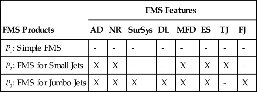
As examples, three types of FMSs are defined in Table 9.1 via their feature configurations. The “X” sign marks selected features, “-” is used for deselected ones.
Table 9.1
Three FMS Products Defined by Their Feature Selections
| FMS Products | FMS Features | |||||||
| AD | NR | SurSys | DL | MFD | ES | TJ | FJ | |
| P1: Simple FMS | - | - | - | - | - | - | - | - |
| P2: FMS for Small Jets | X | X | - | - | X | X | X | - |
| P3: FMS for Jumbo Jets | X | X | X | X | X | X | - | X |
The feature model can be used to control the variability in the other models (application, resource, deployment models) by the definition of relations between the features and the corresponding elements of the other models. This feature mapping can be defined by configuration rules that are assigned to the model’s elements. In the example models of Sections 9.3.2 and 9.4.3, the rules are shown as Boolean expressions that contain the features of the feature model and are attached to the corresponding model elements. The effect is that the selection of some feature induces a selection in all variation points in the related models that are related to this feature. Beyond the abstraction from the model structure, this yields another very useful abstraction mechanism to reduce complexity of variability. In order to be consistent, the relations must respect the modeled variability in the other models.
The relations of the feature model to the other models also define the model configuration, that is, the derivation of a configured model (without variation points) from the configurable, generic model (that contains variation points). Provided that the relations between the feature model and the other models cover all variation points, all variation points can be resolved in this way. Thus, for each complete selection of features (i.e., when every feature in the feature model is either selected or deselected), we obtain a configured model that no longer contains, that is, the variability has been bound and resolved by feature configuration.
9.2.2 Quality assurance of configurable systems
In the setting of a model-based development process, quality assurance is based on the evaluation of the models that represent the design decisions drawn so far in the process. This might either be an evaluation that is explicitly performed after the model has been created in order to prove that the quality requirements are still respected, or it may be an evaluation that is built into the construction of the model, for instance, when the model construction is machine-supported.
Given the framework described above—an overall model, a feature model, the feature-model-relations, and the model configuration mechanism based on feature selections—we discuss now how quality attributes of configurable systems can be evaluated.
Suppose a method is given that allows the evaluation of a model without variation points. In general, there are two possibilities to extend this method to a model with variation points:
1. Product-centered approaches evaluate all product models or a representative subset of them by
a. deriving all (or sufficiently many) product models.
b. evaluating each model.
c. condensing the results to an evaluation of the product line.
2. Product-line-centered approaches extend the method to the evaluation of variation points, that is, they define how to integrate for example, options, alternatives, and parameters into the evaluation without resolving single product variants.
It should be noted that the evaluation criteria on the product line level may slightly differ from those on the product level. In other words, an optimal solution for the product line does not necessarily consist of optimal solutions for every single product.
Product-centered and product-line-centered approaches are illustrated in a schematic diagram in Figure 9.2. The lower layer in the figure, the product model level, represents single system evaluations: A variability-free product model ModelP is evaluated by the function evaluateP. The result of this evaluation is denoted by ResultP.

The upper layer in Figure 9.2, the product line model level, shows the variability-aware function evaluatePL, which is used to analyze the product line model ModelPL and produces the corresponding result ResultPL. The product line model ModelPL includes a feature model that exhibits the supported variability of the product line, base models that represent the realization of the product line (e.g., design models) as well as the mapping model between the feature model and the base models in order to specify the presence conditions of base model’s elements by features.
The function deriveModel denotes the derivation of a product model ModelP from the product line model ModelPL for the feature configuration corresponding to product P. Analogously, deriveResult represents the derivation of a product result from the product line result. The arrow set labeled aggregateResults stands for the inverse operation of aggregating the set of all product results ResultP and building the single product-line result ResultPL.
9.2.2.1 Product-centered approaches
Product-centered approaches start with the product line model ModelPL and create the product models ModelP with the derivation operator deriveModel. Then the evaluation method evaluateP is applied to each ModelP. To get the result ResultPL on the product-line model level, the operator aggregateResults is applied on the set of the individual results ResultP. The representation of ResultPL (and with it the definition of aggregateResults) depends on the concrete evaluation method. This enumerative way of the evaluation of a product line, that is, the consecutive evaluation of each single product, is sometimes called naive (von Rhein et al., 2013) because the number of (potentially) possible product variants to be analyzed are usually too large to be of practical use. Even for a small product line (e.g., option to choose from 10 freely selectable features already results in 1024 possible product variants). Furthermore, the method is inefficient because of redundant computations that result from not exploiting the commonalities between the single products.
9.2.2.2 Product-line-centered approaches
Product-line-centered approaches avoid the creation of single product models, that is, an evaluation method evaluatePL is directly applied to the product line model. The definition of the evaluation method needs to take into account the variability in ModelPL. It is supposed to be more efficient because it is aware of the commonality in the product line. However, its definition is more challenging because of the additional complexity introduced by the variability.
Between these two extremes, there are approaches that reuse analysis methods on product level, but minimize the numbers and the volume of models ModelP, either by selecting a representative subset of products (as done in the product-centered MBT approach in Section 9.3.4 by using a feature coverage criterion) or by reducing the projected models ModelP to representative sub models, cf. for example, sample-based and feature-based methods (Thüm et al., 2012; von Rhein et al., 2013).
We have given the theoretical framework for quality assurance approaches in the context of product lines. Next, we instantiate the framework using two examples of quality assurance techniques. First, we demonstrate how configurable systems can be tested by model-based approaches in order to ensure the correctness of the single product variants (Section 9.3). Second, we discuss how the deployment of application components onto resources can be correctly constructed for configurable systems. We use the “correctness by construction” approach (Chapman, 2006) for the deployment in order to ensure safety constraints (Section 9.4).
9.3 Model-Based Product Line Testing
In this section, we describe how to apply MBT for configurable systems using the schema depicted in Figure 9.2. For that, we first give an introduction to the basic concepts of MBT. Afterwards, we describe the approach of applying this technique on the product model level. Subsequently, we show how to apply it on the product line model level.
9.3.1 What is MBT?
Testing is a widespread means of quality assurance (Ammann and Offutt, 2008; Beizer, 1990; Myers, 1979). The idea is to compare the system under test to a specification by systematically stimulating the system and comparing the observed system behavior to the specified one. The basic approach is to first design test cases based on requirements and to execute them on the system under test afterwards. Complete testing is usually impossible due to loops and a large input data space. So, heuristics like coverage criteria are used to make a quantified statement about the relative quality of the test suite. It has been experienced in many projects that the costs for testing range between 20 and 50% of the overall system engineering costs. This is substantiated by our experiences with industrial transfer projects. For safety-critical systems, testing costs can easily reach up to 80% (Jones, 1991). Nolan et al. (2011) discovered on the basis of data collected at Rolls-Royce that around 52% of the total development effort is spent on verification and validation activities (V&V). They argue that applying a software product line approach will reduce development efforts, but not necessarily the efforts for V&V. They report that V&V can comprise up to 72% of a product’s overall effort in a software product line context, and it could theoretically increase to more than 90% in cases of very low costs because of high reuse. They conclude that “the percentage is higher on a product line not because verification has increased but because the development effort has decreased making verification costs higher in relation to the overall effort,” and that “testability therefore becomes critical for safety-critical product lines.”
Thus, automation is a means to reduce these costs. It can be applied to test execution and to test design. Automating the test design is often implemented by deriving a formal model from requirements and by using test generators that produce a set of test cases based on this model. Corresponding approaches are also called model-based testing (Utting and Legeard, 2006; Zander et al., 2011). There are many different approaches with respect to the chosen modeling language, the modeled aspects of the system, and the algorithms for test generation (Utting et al., 2012).
In the following, we use state machines as defined in Unified Modeling Language (UML) (OMG, 2011) to describe the behavior that is used for test design. We additionally annotate the state machines with variability information and configuration rules in order to use the state machine as the base model for the MBT of product lines. There are several approaches to steer the test generation on the model level (Chilenski and Miller, 1994; Rajan et al., 2008; Weißleder, 2010). We will focus on the widespread approach of applying coverage criteria to the state machine level, for example, such as transition coverage. This criterion defines a type of model elements (here: all transitions of the model) that have to be covered by the generated test cases. There are also coverage criteria for feature models describing the coverage of feature selections and their combinations in the tested products.
9.3.2 Test model for the flight management system
For MBT it is necessary to use models from which test cases can be automatically generated. For our FMS example, we model the application behavior of the FMS product line as a configurable UML state machine. It describes the potential behavior of all products. By including and excluding elements of this model, it can be tailored to describe the behavior of only one product.
The UML state machine is related to the feature model in order to extract product-specific variants of the state machine according to a certain configuration. All variable elements of the state machine have been assigned with a configuration rule consisting of elements of the feature model. Configuration rules define the conditions when those elements need to be included in or excluded from state machine.
By selecting a certain product variant on the feature level (e.g., the defined products in Table 9.1), the corresponding state machine for test generation can be automatically derived using the feature mapping (i.e., by interpretation of the configuration rules).
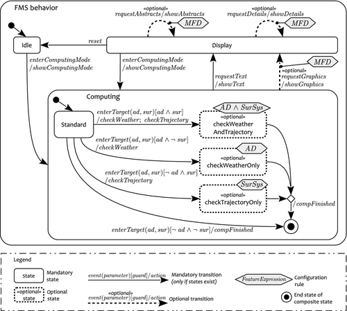
Figure 9.3 shows the configurable state machine for the FMS as well as the configuration rules using the features from the feature model in Figure 9.1. Variation points have been explicitly marked in the state machine. For example, the transition requestGraphics/showGraphics between the states computing and display is only present in a product that has the MFD feature. Usually, the configuration rule can be any Boolean expression using features as predicates. In case of an optional state (e.g., checkTrajectoryOnly), all transitions to or from this state are removed from the state machine if the state’s configuration rule has not been satisfied by the corresponding configuration (e.g., if feature SurSys has been deselected). Thus, those transitions need not be explicitly marked as optional because they depend on the existence of the states. For the sake of simplicity, we have not modeled the complete behavior in the given state machine. Also, not every feature from the feature model has been used here.
We have sketched here how to design product line models for the test generation using the 150% product line modeling approach and how to link them with the feature models. However, this only describes the static connection between the different modeling artifacts. As the framework in Figure 9.2 already depicts, there are several ways of using this information for test design automation of product lines which is explained in the following.
9.3.3 Applying MBT
We now instantiate the basic framework for quality assurance of configurable systems (see Section 9.2.2) for MBT. We show how MBT can be done for product-centered as well as for product-line-centered approaches. Before going into the details of both approaches, we instantiate the framework’s artifacts in Figure 9.2 for the MBT context.
The product line model ModelPL is the union of the feature model, the base model (i.e., the state machine), and the mapping between the features and base model elements as sketched in Section 9.3.2. Each Modeli consists of a concrete product variant (i.e., a feature model configuration, cf. Table 9.2) and the correspondingly resolved model, that is, a state machine that describes the behavior of product i only.
Table 9.2
Representative FMS Products for the Product-Centered MBT Approach
| FMS Products | FMS Features | |||||||
| AD | NR | SurSys | DL | MFD | ES | TJ | FJ | |
| Test suite 1 | X | (?) | X | (?) | X | (?) | (?) | (?) |
| Test suite 2 | - | (?) | - | (?) | - | (?) | (?) | (?) |
The direct result of test generation is the set of generated test cases. Thus, Resulti describes the result for just one product. More interesting information, for example, about transition coverage, can be derived for each product. But what is the meaning of a test case on the product line model level? How should ResultPL—the result of the test generation on the product line model level—be represented? There are several possible forms of test case representations on the product line model level.
One extreme form is a direct mapping of product variants to test cases. This solution conforms to a product-wise description and does not show information on the product line model level. The opposite extreme form consists of a direct mapping from single features to test cases. Given that single test cases usually require information about more than one feature inclusion, this approach is not practicable. The form between both extremes is a mapping from feature configurations (i.e., the inclusion or exclusion of some but not all features) to test cases (see, e.g., Table 9.3 below). This solution allows describing the links between test cases and necessarily included or excluded features. Not making any assumptions about features that are unimportant for the test case allows for optimizing the inclusion of concrete product variants for testing. Summing up, ResultPL is the set of pairs consisting each of a feature configuration and a set of corresponding test cases.
Table 9.3
Required Configurations for the Generated Test Cases in the Product-Line-Centered MBT Approach
| Test Candidates | Test Cases | FMS Features | |||||||
| AD | NR | SurSys | DL | MFD | ES | TJ | FJ | ||
| Candidate 1 | TC1, TC2, TC3, TC4, TC5, TC6, TC7, TC8 | ? | (?) | ? | (?) | ? | (?) | (?) | (?) |
| Candidate 2 | TC5 | X | (?) | ? | (?) | ? | (?) | (?) | (?) |
| Candidate 3 | TC9 | X | (?) | X | (?) | ? | (?) | (?) | (?) |
In the following, we describe the two mentioned approaches for test generation for configurable systems. The two approaches are focused on different sequences of applying coverage criteria for test case selection on the different test artifacts. Both approaches have been implemented in our prototypical tool chain SPLTestbench. The product-centered approach consists of a concatenation of well-known techniques. Consequently, it uses parts of the available information in a step-wise manner. The product-line-centered approach is aimed at combining all techniques in one step. Thus, by using all available information in one step, it bears the potential for an improved quality of the generated artifacts.
9.3.4 Product-centered MBT
Here, we describe the product-centered approach for MBT of configurable systems. This approach consists of three steps, each of which uses one of the three available sources—the feature model, the base model, and feature mapping. In the first step, a representative set of products is derived using feature configurations. This can be done, for example, by applying heuristics such as feature-model-based coverage criteria (Oster et al., 2011). For our FMS example, we use the feature-based coverage criterion All-Features-Included-And-Excluded, which is satisfied by a set of feature configurations if each non-mandatory feature is at least once included and at least once excluded. Feature configuration generation with SPLTestbench results in two relevant feature configurations (regarding only the features used in the state machine in Figure 9.3). See Table 9.2: The first test candidate is equipped with all features used in the state machine; the second candidate is the minimal FMS product consisting of the mandatory features only. The “(?)” sign in the table denotes features that are irrelevant for the test cases, because they have not been used in the FMS state machine example.
In the second step, the feature mapping is used to derive a resolved state machine model for each configured product variant.
The third step consists of running automated model-based test generation on each of the resolved state machines. There are several influencing factors for model-based test generation (cf. Weißleder, 2009). However, we focus on generating test suites that cover all transitions of each resolved state machine. For All-Features-Included-And-Excluded, satisfying transition coverage results in two test suites with a total number of 12 test cases and 63 test steps.
The product-centered approach can be implemented by standard test generators. This implementation is straightforward. It suffers, however, from the disadvantage that the available information is not used together at once, but in sequence. One consequence of this sequential use of information is that sets of model elements that are common to several product variants are tested again and again for each variant in full detail. While this repetitive approach might be useful for testing single products, it results in unnecessarily high effort for product line approaches that apply the reuse of system artifacts. Another consequence of this sequential approach is that the test effort cannot be focused on the variability. Each product variant is handled separately and the knowledge about the commonalities in their state machines is unused.
9.3.5 Product-line-centered MBT
Here, we describe the product-line-centered approach for MBT of configurable systems. In contrast to the product-centered approach, it is focused on using all available information together at once and not in sequence.
For implementing this approach, one typically has two options: The first choice is the invention of a new test generator; the second is an appropriate transformation of the input model. Our approach is based on the latter, that is, we use a model transformation to combine all the available information within one model. By ensuring that the model transformation results in a valid instance of UML state machines, we take advantage of using existing test generators that can be applied on this combined model.
Our model transformation works as follows: The information from the feature model and the feature mapping is used to extend the transitions of the state machine. This extension alters transitions in a way that a transition can only be fired if the features of its configuration rule have not been excluded yet. Figure 9.4 shows the result of an exemplary transformation of a transition that originally had only the guard [Guard] and no effect. The transformation adds two variables for each feature f: The variable valueFeaturef marks the value of the feature selection. The variable isSetFeaturef marks whether the value of the feature has been set already (i.e., if it has been already bound before). A transition that is mapped to a feature can be fired only if the feature has been included in the product variant already (i.e., if valueFeature == true) or if the feature has not been considered at all (i.e., if isSetFeaturef == false). As the effect of the transition, both values are set to true. This means that for the current path in the model, this variable assignment cannot be undone in order to guarantee consistency of the product feature selection. For more complex configuration rules, there are corresponding transformations.
As a consequence of this transformation, the test generator only generates paths through the state machine for which there is at least one valid product variant. Furthermore, the test generator not only generates a set of paths, but also the conditions for the corresponding valid products on the feature model level (i.e. in form of feature configurations). This allows assigning the generated test cases to the product variants they are run on.
We have applied the transformation on our FMS example. The transformed state machine was used then to generate tests to satisfy transition coverage. As a result, nine test cases with a total number of 47 external steps were generated that covered all transitions. The generated test cases are shown as message sequence charts in Figure 9.5. Each test case is assigned with only the necessarily included or excluded features to make this test executable. This leaves room for optimization of the test suites such as, for example, deriving a big or small number of variants or maximizing a certain coverage criterion on the feature model. The corresponding minimal configurations for the test cases are shown in Table 9.3. The sign “(?)” denotes the features that have not been needed to be bound for running the test case. “(?)” again marks features not used in the statechart.
9.3.6 Comparison
Here, we describe a first comparison of both approaches. Our comparison uses two values: coverage criteria and the efficiency of the test suite to satisfy them. The application of coverage criteria is a widely accepted means to measure the quality of test suites, which is also recommended by standards for safety-critical systems such as the ISO 61508. We measure the test suite efficiency in terms of the numbers of test cases and test steps. The more efficient we consider the test suite, the fewer test cases and test steps are needed to satisfy a certain coverage criterion.
The current results of our evaluations are that both approaches achieve the same degree of base model coverage, which is 100% transition coverage. Furthermore, the product-line-centered approach needed only 9 test cases with a total length of 47 test steps compared to 12 test cases and 63 test steps of the product-centered approach. Based on these results, the product-line-centered approach seems to produce a more efficient test suite than the product-centered approach while guaranteeing the same degree of base model coverage.
For future work, we plan to further investigate the relations of coverage criteria on feature models and base models. For instance, there are other criteria at the feature model level such as All-Feature-Pairs (Oster et al., 2011). The product-centered approach is able to make a quantifiable statement about feature model coverage. Applying the All-Feature-Pairs-and-All-Transitions coverage criteria instead of the All-Feature-Included-And-Excluded-and-All-Transitions coverage in the product-centered approach have resulted in larger test suites: Testing of the FMS product line would need 6 test suites (i.e. 6 product variants) with a total number of 36 test cases and 185 test steps.
The product-line-centered approach leaves feature model coverage to the last optimization step without guaranteeing a certain degree of coverage. The meaning of feature model coverage is not yet clear here. But the most important thing to do is to test specified behavior. And the resulting question is about the impact of the feature model on testing the described behavior.
9.4 Model-Based Deployment
As second example of the extension of a quality assurance technique to configurable systems, we now discuss model-based deployment. A deployment model describes how the resources of a system are employed to execute the application functions. Beyond the capabilities of the resources, it is the deployment that essentially determines the runtime properties of the system, such as responsiveness, reliability, and availability. The automatic or machine-supported design of a deployment can be used to ensure the corresponding runtime qualities by construction. For that purpose the requirements specifying these qualities are fed into a deployment model builder that constructs one or proposes several deployment models that guarantee the required qualities. Such a deployment model builder for many-core systems, for instance, is described in Hilbrich (2012). In this section we discuss how a deployment model builder can be extended to systems with configurable applications and resources.
9.4.1 What is deployment?
Deployment is an important task within the design phase of a systems engineering process. It is concerned with the assignment of resources, for example, CPU time, memory, or access to I/O adapters for application components. The design artifact that is produced by this engineering step is referred to as a deployment model. With resource capabilities of the hardware, network, and computing components on the one hand and resource demands of the application components on the other, the deployment acts as central resource broker. A deployment is often subject to a variety of general and domain-specific constraints which determine its correctness. Generally speaking, a deployment is correct if it assigns the proper type and amount of resources to all application components at any moment during runtime of the system. It is the job of the operating system to ensure the integrity of the deployment at runtime by means of scheduling and isolation techniques.
Due to the complexity of these constraints and the intricacy of the application and resource architectures found in current software-intensive embedded systems, constructing a correct deployment is of NP-complexity. This renders a manual construction a time-consuming and error-prone task. Still, a correct deployment is an essential prerequisite for achieving high levels of system quality because it has a direct impact on the fulfillment of major system requirements. This is especially true for extra-functional requirements of embedded software, such as real-time behavior, safety, and reliability requirements. For instance, a faulty resource assignment may lead to non-deterministic latencies when a resource is erroneously “overbooked,” which may eventually jeopardize the real-time behavior of the entire system.
Beyond its relevance for the fulfillment of extra-functional requirements, a deployment also helps to determine the amount of resources, for example, processing power or memory capacity, which are required. Often it is the starting point for extensive optimizations on the system level because it has direct impact on the cost and performance of the system to be built. A deployment model builder supports the optimization by providing scores for the deployments it constructs. Depending on the quality requirements and evaluation criteria that are given to the deployment model builder, it applies metrics that evaluate the deployments with respect to these requirements and criteria. The results ri can be weighted with user defined weights wi, which finally defines the score of a deployment D:

Evaluation criteria may encompass a variety of domain-specific and application-specific aspects of a system architecture, such as hardware cost, penalties for unused capacities, or the load distribution. The construction of a deployment therefore is not only applied to produce correct resource assignments, but it is also a vital part of the design space exploration process to find (cost-)optimal resource designs.
In addition to the relevance of a deployment for the correctness and quality of the system, it is also a central asset and synchronization point for distributed development teams. With the trend toward integrating more and more software components from different vendors into a single electronic control unit, a correct deployment proves to be an essential design artifact to prevent surprises during the integration phase.
9.4.2 Spatial and temporal deployment
In consideration of its NP-complexity, the construction of a deployment should be subdivided into a spatial and a temporal part. A spatial deployment focuses on the entire system architecture and yields a mapping from application components to resources. It is constrained not only by the amount and type of the resources available, but also by safety and reliability requirements. A spatial deployment determines which resources are exclusively used by some application component and which resources have to be shared.
Coordinating the access to shared resources in the temporal dimension is the objective of the temporal deployment. It addresses the question of when to execute an application component on a shared resource, so that all real-time requirements are met. Usually, a static schedule, which correctly executes all application components using shared resources, is produced as a result of a temporal deployment.
Figure 9.6 depicts a common process model for the construction of a deployment model. The spatial deployment should be conducted first because it determines a major part of the system architecture and its properties. However, it is only feasible if a correct temporal deployment can also be constructed. Otherwise, the spatial deployment has to be modified to facilitate a temporal deployment.

In this contribution, we focus on the spatial deployment and its extension to configurable systems. Schedulability tests and tools for generating static schedules for a temporal deployment have also been extensively studied (see Section 9.5).
Their extension to configurable systems, however, is an issue for further research, which might be undertaken using the framework we present here.
9.4.3 Application and resource models for the flight management system
In order to construct a deployment model for the FMS, we first have to provide a resource model. Second, we have to extend the application model by the resource demands of the application components. An extract of the latter is illustrated in Figure 9.7. It shows three of the application components and their resource requirements. In order to simplify matters, we assume that each feature in our feature model (see Figure 9.1) is realized by a single application component. This defines the relation of the feature model and the application model, that is, the feature mapping. Furthermore, resource requirements and safety requirements are assigned to each application component. These requirements constrain the spatial deployment and define the valid assignments of application components to resources.
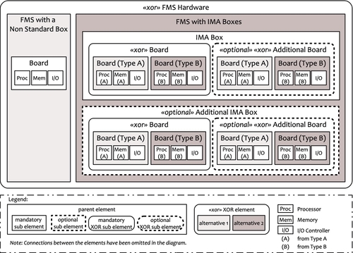
A simplified resource model is depicted in Figure 9.8. Basically, a FMS may either be built as a single, non-standard, stand-alone unit, or it may use a set of standardized IMA boxes with IMA processing boards. For our example, we assume that in the second case either one or two IMA boxes can be used. Each IMA box may host either one or two processing boards. There are two kinds of processing boards available: type A and type B. The board types differ in their processor (architecture type, vendor, and performance) and in the size of the included memory. Type A boards feature larger memories and faster processors. Boards with type B, on the other hand, are equipped with less memory and slower processors, but they are also less expensive.
At this point we do not define a relation between the variance points of the resource model and the features for two reasons. First, the deployment model that is now constructed induces a feature-to-resource relation by extending the feature-to-application relation with the application-to-resource relation defined by the deployment model. In this induced feature-to-resource relation a resource model element is related to a feature if there is an application model element that is (1) related to the feature and (2) deployed onto the resource model element.
Second, the resource variants are obviously not induced directly by the features we considered for the application. This is indeed a typical situation. Different parts of the system are designed with respect to different specific requirements, constraints, and features. For example, the variance drivers for the resources might be induced by supplier relations, future availability, costs, or other factors that have nothing to do with the functionality of the system. It was possible to represent this as an additional, resource-specific feature model. There is another issue here, however. In fact, the resource variants in this case represent design space alternatives rather than system variants. From the design space alternatives one or several candidates are selected for the realization of the application. The other ones are withdrawn. This is different from the variants of the application: They are all required and must all be realized.
The result of the construction of the deployment model in our example correspondingly consists of two parts: a reduction of the variance of the resource model and a feature mapping to the remaining resource model that is given by the composition of the feature mapping to the application model and the deployment model.
In Figure 9.2 we introduced our general concept for the evaluation of configurable systems. We now apply this general concept to the construction of a deployment of the FMS example and describe a product-centered and a product-line-centered approach for this engineering challenge.
9.4.4 Product-centered software deployment
The product-centered approach consists of three basic steps. First, sufficiently many product models are derived from product line model. These products are then individually evaluated by the deployment model builder in a second step. Finally, the results obtained from these evaluations are aggregated and combined, so that an assessment of the entire product line is achieved. In the following, these steps will be described in more detail in the context of our FMS example.
9.4.4.1 Step 1: Deriving the product models
A product model is the combination of an application model, a resource model, and a deployment model. For the construction of the deployment model, the application model and the resource model must be given. So we assume to have an application model with variation points and a resource model with variation points as discussed in the previous section. In order to apply the deployment model builder (which only works for models without variation points), we have to derive all combinations of application product models and resource product models.
9.4.4.2 Step 2: Evaluating the deployment candidates
Each pair of a variance-free application model and a variance-free resource model can be supplied to the deployment model builder, which either constructs a deployment for this pair that satisfies all resource requirements and safety requirements or it indicates that no valid deployment can be found. In the latter case, the resource model is deleted from the list of possible resource candidates for this application configuration. As mentioned above, the deployment model builder also attaches a score to each deployment candidate it finds. These will be used in Step 3 to find the product line deployment. Note that all deployment candidates constructed in this way are correct, but not necessarily optimal designs for the overall configurable system.
Already, our small example has many product models, that is, pairs of configured application and resource models. So, we do not compute the whole set of pairs. Instead we use subsets of viable candidates, which is also the way one would proceed practically. There are often external criteria, obtained, for instance, from market surveys, supplier relations, or production constraints, which indicate some configurations as viable, whereas others are excluded from further consideration.
For our example we consider only three different types of flight management applications (products) that have to be developed: Simple FMS, FMS for Small Jets, and FMS for Jumbo Jets. These products and their features have been defined in Table 9.1.
Concerning the possible resource configurations, assume that the following set of viable variants is defined based on the resource model in Figure 9.8. Table 9.4 lists these variants together with their relative hardware cost factor, which is used as a quality evaluation criterion. Only these resource variants shall be considered as candidates for the deployment of the application and to realize the envisioned product line of FMSs.
Table 9.4
Several Variants of the Resource Architecture
| Resource Variants | Resource Components | Relative Cost |
| HWV0 | 1 Non-standard Box | 1 |
| HWV1 | 1 IMA Box with 2 Boards Type B | 10 |
| HWV2 | 1 IMA Box with 2 Boards Type A | 15 |
| HWV3 | 2 IMA Boxes, each with 2 Boards Type A | 30 |
The result of the deployment model builder for this restricted set of application and resource variants might look as represented in Table 9.5. The numbers indicate the scores that are given to the application and resource pairs by the deployment model builder. The empty set (∅) is used to characterize a pair without a valid deployment.
Table 9.5
Scores of Optimal Product Candidates for All Resource and Application Combinations
| FMS Products (Application Variants) | Resource Variants | |||
| HWV0 | HWV1 | HWV2 | HWV3 | |
| Simple FMS | 100 | 75 | 65 | 35 |
| FMS for Small Jets | Ø | 95 | 90 | 45 |
| FMS for Jumbo Jets | Ø | Ø | Ø | 75 |

For the Simple FMS, the stand-alone unit (HWV0) is clearly an optimal choice with a score of 100. The other resource configurations for the Simple FMS are still viable, but they use significantly more resources, which will not be fully utilized and result in lower scores.
However, the HWV0 is not a viable choice for the FMS for Small Jets as its AirData software component requires a 2x redundant execution, which the stand-alone unit cannot provide. Score differences between HWV1 and HWV2 result from different costs for the processing boards of type A and type B. Similarly, the FMS for Jumbo Jets can only be realized with HWV3, because the Surveillance System requires a 4x redundant execution.
The description of the first two steps illustrates the challenge of dealing with the combinatorial explosion in the product-centered development approach. Finding and assessing all viable product candidates exceeds the capabilities of a manual development—even for simple systems with few variation points. Instead, a tool-supported approach is required to automate these engineering steps. In Hilbrich and Dieudonne (2013), Hilbrich (2012), and van Kampenhout and Hilbrich (2013) we presented a tool that is able to construct an optimal deployment and facilitate Step 1 and Step 2.
9.4.4.3 Step 3: Aggregation of results
In the next step, the results from Table 9.5 have to be aggregated and combined to a deployment model for the configurable application and resource models. Instead of a formal definition of an aggregation, we discuss informally how the results of Table 9.5 for the individual application and resource model pairs without variation points can be interpreted and used to build a single, configurable deployment
The application level has already been modeled as a product line and related to the feature model as presented in Figure 9.1. The initially provided set of possible resource configurations from Figure 9.8 now can be further refined using the results of the deployment model builder. For instance, variant HWV2 appears to be a suboptimal choice for all FMS products. Therefore, it may be removed from the set of viable resource variants.
However, a systems engineer may decide to use HWV2 for the implementation the FMS for Small Jets product ![]() instead of HWV1. This choice would allow for more homogeneity in the hardware components of the entire product line, because processing boards of type B would no longer be required. Taking into account this criterion implies that although using HWV1 is a locally optimal choice for
instead of HWV1. This choice would allow for more homogeneity in the hardware components of the entire product line, because processing boards of type B would no longer be required. Taking into account this criterion implies that although using HWV1 is a locally optimal choice for ![]() , the decision to use resource variant HWV2 for
, the decision to use resource variant HWV2 for ![]() instead is a globally optimal choice for the entire product line and may be preferred by the systems engineer.
instead is a globally optimal choice for the entire product line and may be preferred by the systems engineer.
This aggregation of deployments based on their scores and the homogeneity criterion yields the following configurable deployment for the whole product line. First, the resource model is reduced. The boards of Type B are deleted, the XOR-boards that contained the alternative boards of Type A and Type B are replaced by the remaining boards of Type A. Inside the FMS with IMA Boxes we have thus the IMA Box with one Board of Type A and an optional. Additional Board of Type A, and the optional Additional IMA Box with the same internal structure.
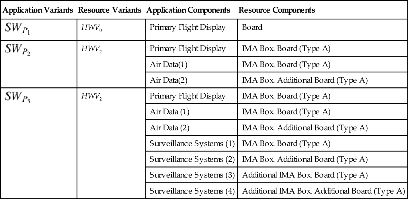
The corresponding deployments of the three individual applications are given in Table 9.6. The additional numbers behind the application components indicate their redundant copies that are deployed to different resource components.
Table 9.6
Product Deployments to the Reduced Resources
| Application Variants | Resource Variants | Application Components | Resource Components |
| HWV0 | Primary Flight Display | Board | |
| HWV2 | Primary Flight Display | IMA Box. Board (Type A) | |
| Air Data(1) | IMA Box. Board (Type A) | ||
| Air Data(2) | IMA Box. Additional Board (Type A) | ||
| HWV2 | Primary Flight Display | IMA Box. Board (Type A) | |
| Air Data (1) | IMA Box. Board (Type A) | ||
| Air Data (2) | IMA Box. Additional Board (Type A) | ||
| Surveillance Systems (1) | IMA Box. Board (Type A) | ||
| Surveillance Systems (2) | IMA Box. Additional Board (Type A) | ||
| Surveillance Systems (3) | Additional IMA Box. Board (Type A) | ||
| Surveillance Systems (4) | Additional IMA Box. Additional Board (Type A) |
The mapping defined by the deployment, combined with the feature mapping to the application model, yields the feature mapping indicated in Table 9.7.
9.4.5 Product-line-centered software deployment
Deriving all possible products may be a very time-consuming and expensive approach for large and complex systems with many variation points. For some systems, it may not even be a viable approach at all. In these situations, optimization strategies and heuristics are needed that focus more on the product line instead of deriving all individual products. The following two strategies may be beneficial in these situations.
9.4.5.1 Reuse of previously computed allocations
The first strategy is based on the assumption that it is not feasible to find and evaluate all deployments for each application and resource pair. Instead, it is assumed that finding just one valid deployment for each pair (S,H) would be sufficient. The search for one deployment can be optimized by reusing parts of a previously computed deployment.
For this purpose, we start with a minimum product containing only mandatory application and resource components. The minimum product is then used to find a minimum deployment for the set of all mandatory application components. All other products with optional application components may then reuse this minimum deployment as a starting point when searching for a valid deployment.
In a best-case scenario, only the deployments for optional application components need to be constructed and there are no changes to the minimum deployment necessary. In the worst-case scenario, the selection of optional application components invalidates the entire minimum deployment, so that a reuse is not possible.
This approach still considers all application and resource combinations, so that its optimization potential for large system is limited.
9.4.5.2 Maximum approach
In contrast to the previous heuristic, this strategy is based on a maximum deployment. For this purpose, all optional application and resource components are assumed to be selected. Alternative application components and their requirements may be coarsened into a single application component with a superset of the requirements of all previously alternative application components. Alternative resource components, on the other hand, can be coarsened as well. This can be done by creating a single resource component instead that contains a set of resource capacities provided by all alternatives. The resulting application and resource architectures no longer contain any variability. They can then be used to compute a maximum deployment.
In order to retrieve the deployment for each individual product, the feature model is used to selectively remove application components from the system architecture. The resulting deployment of application components is still correct, but it may no longer be optimal and resource-efficient. The removal of application components may also result in entirely unused resources. These resources may be removed from the resource architecture for a specific product in order to improve its resource-efficiency.
This approach does not consider all resource and application combinations.
Therefore, it may not lead to optimal system architectures. For instance, in the FMS example, this approach would not try to use the stand-alone unit, just because it would not be sufficient for the FMS for Jumbo Jets product. The approach of coarsening the system architecture allows for significant process efficiency improvements, but at the cost of achieving less optimal solutions.
9.5 Related Work
In the following we give an overview on related work with respect to product line evaluations in general, product line testing approaches, and approaches for software deployment.
9.5.1 General product line approaches
Beyond the basic product line modeling concepts presented in this chapter are many other approaches that we briefly sketch. They differ in how they represent variability within the various system models, whether they provide explicitly defined variability concepts in the models, and which kind of relationships between feature and system models they allow. In Voelter and Groher (2007), product line approaches have been distinguished in approaches using negative versus positive variability. An example of negative variability approaches is 150% modeling (Czarnecki and Antkiewicz, 2005; Heidenreich et al., 2008; Mann and Rock, 2009). The system models represent so-called 150% models as the base models of the product line and include all the supported variability. Options or alternatives that have been not selected for a specific product will be removed from the base models. In this chapter we have also used a 150% modeling approach. Examples for positive variability approaches are given in Apel and Kästner (2009) and Thaker et al. (2007). Here, a base model exhibits basic features only. A number of transformations are performed on the base model to add specific features and to gain the product-specific variants. Delta modeling (Clarke et al., 2010) can be used for both positive and negative variability. A general syntactic framework for product line artifacts is suggested by the common variability language CVL (OMG, 2012).
A precondition for the quality assurance of single products as well as of the complete product line is that the engineering artifacts have been consistently set up with respect to the variability dimension. Analysis and assessment methods have been developed for the various models in product line engineering approaches. The interpretation of feature models as logical formulas to be used by theorem provers, SAT solvers, or other formal reasoning have been introduced in Batory (2005) and Zhang et al. (2004), for example. A literature overview of the use of such automated analysis of feature models is given in Benavides et al. (2010). Our work is based on this because we need the ability to compute correct feature configurations for the feature coverage criterion and for the model transformations of configurable state machines in order to use standard test generators, for instance.
The idea to make the transition from single evaluation methods to variability-aware methods because of efficiency issues has been already identified within the product line community. An overview of published product-centered and product-line-centered analysis approaches is given in von Rhein et al. (2013) and Thüm et al. (2012). The authors provide a classification model in order to compare these approaches. Their model distinguishes between the dimensions of sampling, feature grouping, and variability encoding. Sampling is about which products will be selected for analysis; feature grouping is about which feature combinations will be selected; and the variability encoding represents the dimension concerning whether analysis methods are able to deal with explicit variability information.
A literature overview of approaches that consider the variability of quality attributes within a product line is given in Myllärniemi et al. (2012). The focus is set on why, how, and which quality attributes vary within a product line.
9.5.2 Product line testing
Testing is discussed in many scientific articles, experience reports, and books (Ammann and Offutt, 2008; Beizer, 1990; Binder, 1999). As testing usually requires much effort during system engineering, there is a trend toward reducing test costs by applying test automation. There are several approaches of test automation for test design and test execution. We focus on automated test design. Some well-known approaches in this area are data-driven or action word-driven testing that strive to use abstract elements in the test design that can be replaced by several concrete elements representing, for example, several data values or action words. The most efficient technique in this respect is MBT, which allows the use of any kind of models in order to derive test cases (Utting and Legeard, 2006; Utting et al., 2012; Weißleder, 2009; Zander et al., 2011). Many reports are available dealing with the efficiency and effectiveness of MBT (Forrester Research, 2012; Pretschner, 2005; Pretschner et al., 2005; Weißleder, 2009; Weißleder et al., 2011).
Product lines have to be tested (Lee et al., 2012; McGregor, 2001). Given that product lines can be described using models, the application of MBT is an obvious solution for testing product lines. Several approaches exist for applying MBT to product lines (Weißleder et al., 2008). For instance, coverage criteria can be applied to the feature models to select a representative set of products for testing (Oster et al., 2011). Most approaches in this area, however, are focused on product-centered evaluation approaches, that is, they apply well-known techniques for single products only. We also started the discussion about applying the product-line-centered approach to MBT (Weißleder and Lackner, 2013). Evaluations of this approach are currently under development.
9.5.3 Deployment
Deployment comprises of a spatial and temporal dimension. The temporal deployment of application software has been discussed extensively in the context of scheduling in real-time systems. Analyzing the schedulability of tasks under real-time conditions has been formally described by Liu and Layland (1973). An overview about scheduling algorithms and a variety of heuristics is presented in Buttazzo (2004), Carpenter et al. (2004), Leung et al. (2004), and Pinedo (2008). Offline scheduling approaches, because they are often used in safety-critical systems, are discussed in Baro et al. (2012) and Fohler (1994). Tools for the construction of temporal deployments, that is, static schedules, are described in Brocaly et al. (2010) and Hilbrich and Goltz (2011). A formal approach to analyze the schedulability of real-time objects based on timed automata families is introduced in Sabouri et al. (2012). Their approach fits to our category of product-line-centered approaches. Similar to our product-line-centered MBT approach, the authors transform timed automata to reuse the common state space during schedulability analysis by late decision making for feature bindings.
Spatial deployment and its challenges have been discussed in Taylor et al. (2009). Engineering approaches for a spatial software deployment for safety-critical systems have been investigated in Hilbrich and Dieudonne (2013), Hilbrich (2012), and van Kampenhout and Hilbrich (2013). A deployment of software components based on their energy consumption has been studied in AlEnawy and Aydin (2005). To the best of our knowledge, there are no solutions yet for spatial deployment that deal explicitly with configurability of the application components or the resources.
9.6 Conclusion
Customer-configurable systems stress the fact that manufacturers do not always have the ability to extensively conduct quality assurance measures for each single customer-specific product, but they need to have the confidence that their product line setup will achieve the quality objectives for all those single products. In this chapter, we introduced two primary ways that quality assurance can be established in this context: product-centered approaches and product-line-centered approaches as depicted in Figure 9.2. Furthermore, we pointed out that product-line-centered approaches promise to be more efficient because they can handle directly the explicitly modeled variability and can exploit the commonalities of single configured systems.
To give an idea how such approaches can be set up, we worked out two applications. We presented how the quality of customer-configurable systems can be assured by MBT and by model-based deployment approaches for both ways. This chapter does not thoroughly provide state-of-the-art techniques already usable out of the box, but rather defines research and development paths for the near future as summarized separately for the two presented applications below. The needs for these techniques, however, are very contemporary, as the sketched examples may have shown. Flexible, customer-configurable systems do exist, and high quality is an essential requirement. Thus, systematic methods for the achievement of quality in customer-configurable systems are needed.
9.6.1 Model-based product line testing
For MBT, the results of our example show that an efficiency gain is possible by using all available information together on the product-line-model level compared to the approaches of resolving a representative set of products and applying the technique to each selected product. There are, however, several aspects to discuss about such statements. For instance, there are different means to steer test generation for both approaches.
The test generation on the product-line-model level only requires defining a coverage criterion to satisfy at the base model. In contrast to that, test generation on the product-model level requires defining a coverage criterion on the feature-model level and a coverage criterion on the level of the resolved product model. This results in the obvious difference that the product-centered evaluation is focused on evaluating the quality of each selected product variant thoroughly, and the product-line-centered evaluation is focused on evaluating the behavior of all products. The product-line-centered approach bears the potential advantage of avoiding retesting elements that were already tested in other product variants. The impact of this advantage becomes stronger the more system components were reused during system engineering. If the components were not reused, however, and several product variants are developed from scratch or with a minimal reuse, then the product-centered approach has the advantage of considering all product variants independently.
Conversely, the product-line-centered approach has the potential disadvantage of missing faults that are introduced by a lack of component reuse, and the product-centered approach potentially results in testing all system components again and again in each selected variant. Consequently, the choice of the test generation approach strongly depends on the system engineering approach. This aspect is not always obvious to testers. So, the most important question for testers is whether they want to focus their tests on product line behavior or on covering product variants. A compromise is probably the best solution here.
9.6.2 Model-based deployment for product lines
Concerning deployment, it became apparent that the product-centered approach quickly led to a combinatorial explosion of product candidates. Tools may provide some support to automate the determination and assessment of product candidates. However, the product-centered approach is not a viable way to address the design challenges of a complex product line. Instead, powerful product-line-centered approaches are required. These may comprise strategies and heuristics to improve the efficiency of the computation or reduce the complexity of the variability in the system. Still, further research on product-line-centered approaches is necessary to overcome the shortcomings of the product-centered approaches and allow for complex, software-intensive and configurable systems with high quality.