
3
Reliability Modeling for Systems Engineers: Nonmaintained Systems
3.1 WHAT TO EXPECT FROM THIS CHAPTER
It is not the purpose of this book to support your becoming a reliability engineering specialist. As a systems engineer, though, you will be interacting with these specialists both as a supplier and as a customer. You will be supplying reliability requirements that specialist engineers will use to guide their design for reliability work. You will be a customer for information flowing back from reliability engineering specialists regarding how well a design, in its current state, is likely to meet those reliability requirements and whether deployed systems are meeting their reliability requirements. The purpose of this chapter, then, is primarily to support your supplier and customer roles in these interactions. You will need enough facility with the language and concepts of reliability engineering that you will create sensible reliability requirements. Much of this was covered in Chapter 2, and the material covered in this chapter supports and amplifies the concepts introduced there. You will also need enough of this facility to be able to sensibly use the information provided by specialist reliability engineers so that design may be properly guided.
The material in this chapter is designed to support this latter need. What you will find here is chosen so that it reinforces correct use of the concepts and language of reliability modeling for nonmaintained systems.1 It is complete enough that it covers almost all situations you will normally encounter, and if you learn this well you will be able to adapt it to unusual situations as well. While everything here is precise and in a useful order, no attempt is made to provide mathematical rigor with theorems and proofs even though there is a flourishing mathematical theory of reliability [3, 4] that underpins these ideas. If you wish to follow these developments further, many additional references are provided.
3.2 INTRODUCTION
The industrial, medical, and military systems prevalent today are usually very complex and closely coupled, and expensive and time-consuming to develop. For transparent economic and schedule reasons, it is not even remotely realistic to test such systems for reliability. Indeed, to do so would be to fly in the face of the guiding principle of contemporary systems engineering for the sustainability disciplines: design the system from the earliest stages of its development to incorporate features that promote reliable, maintainable, and supportable operation. In short, in preference to a costly and lengthy testing program, or, worse, design scrap-and-rework, take those actions during systems engineering and design that lead to a sustainable, profitable system.
Accepting, then, that testing a complicated system for reliability is not sensible, what can systems engineers and reliability engineers do to ensure that a system meets the reliability needs of its customers? In this book, we advocate strongly for the discipline of design for reliability, the discipline that encompasses actions that are taken during systems engineering and design to anticipate and prevent failures. Design for reliability is discussed from this point of view in Chapter 6 where we introduce specific methods such as fault tree analysis (FTA), failure modes, effects, and criticality analysis (FMECA), and others that provide systematic, repeatable techniques that are widely applicable and very effective in anticipating the failures that are possible in the system and deploying suitable countermeasures that prevent those failures from occurring. An important part of the design for reliability process is the ability to project or forecast in quantitative terms the reliability one can expect of the system given the current state of the design. A discipline called reliability modeling has been developed to enable these sorts of quantitative projections to be made, even before any of the system may be built (or even prototyped).
Reliability modeling is based on the observation that while the systems we deal with are complex and closely coupled, usually they are made up of a large number of simpler components. Reliability modeling is a process of combining, in suitable mathematical fashion, quantitative information about the reliability of individual components to produce information about the reliability of the complex assembly of those components that is the system in question. It is usually possible to obtain information about the reliability of these simpler components from life testing, fundamental physical principles, and real field experience. Life testing of components is possible because it deals with only one (population of identical) component at a time; complicated interactions with other components are not present, and varying environmental conditions can be applied to characterize the component’s reliability in different environments likely to be encountered in operation [16, 62]. Estimation of component reliability from fundamental physical principles is possible in some cases because the physical, chemical, mechanical, and/or electrical mechanisms causing degradation of the component have been identified in many practical classes of components [10, 24]. Component reliability may also be estimated from real operational experience with systems that contain the component provided that the failure that caused a system to be taken out of service for repair can be traced to that specific component [7, 55] (see also Section 5.6). This chapter is devoted to helping you gain an understanding of reliability modeling for nonmaintained systems so that you are equipped to assess whether your reliability requirements are likely to be met as part of an ongoing process throughout the design and development of the system. Reliability models for nonmaintained systems introduced in this chapter form building blocks for the reliability models for maintained systems discussed in Chapter 4.
However, all the reliability modeling you can afford is of little value unless you use what you learned from it to do one (or both) of two things:
- Improve the reliability of the system if modeling shows that the system in its current configuration is unlikely to meet its reliability requirements.
- Determine that the reliability requirements originally proposed are too restrictive and may be loosened, possibly creating an opportunity for development cost savings.
Chapter 5 discusses comparison of what is learned from reliability modeling (usually called a “reliability prediction”) with the relevant reliability requirement(s). To improve the reliability of the system, additional design for reliability actions must be undertaken or the design for reliability actions already undertaken should be re-examined at greater depth (Chapter 6). The alternative is to decide that the original reliability requirements were more restrictive than they needed to be—but this decision can’t really be made without thorough re-examination of the process by which they were created (QFD, House of Quality, Kano analysis, etc., introduced in Section 1.6.1). Without this response, reliability modeling has little value.
Finally, most systems are intended to be repaired when they fail, and by the repair to be restored to service. There are obvious exceptions, of course (viz., satellites, although the example of the Hubble Space Telescope shows that when the stakes are high enough, truly heroic measures will be undertaken to repair even some systems that are traditionally designated as non-repairable). Many reliability effectiveness criteria are appropriate for describing the frequency and duration of failures of a maintainable system (see Section 4.3). The system maintenance concept (see Chapter 10) tells how the system will be restored to service when it fails, and which part(s) of the system are designated as repaired and which parts are not repaired. A reliability model for the system mirrors the system maintenance plan: the model builds up reliability descriptions of the maintained parts of the system from reliability descriptions of their constituent components and subassemblies. All systems contain some components that are not maintainable in the sense that if a system failure is traceable to one such nonmaintainable component, repair of the system is effected by discarding the failed component and replacing it with another (usually new) one. Some systems also contain more complex subassemblies that may be removed and replaced in order to bring a system back to proper operation and that are sufficiently complex and expensive that the removed units are themselves repaired and used as spare parts for later system repairs. See Chapter 11 for more details on this type of operation. Accordingly, Chapters 3 and 4 are structured so that we learn about reliability effectiveness criteria and models for nonmaintainable components first and then we learn how these are combined to form reliability effectiveness criteria and models for the higher level entries in the system maintenance concept—the subassemblies, line-replaceable units, etc., on up to the system as a whole.
3.3 RELIABILITY EFFECTIVENESS CRITERIA AND FIGURES OF MERIT FOR NONMAINTAINED UNITS
3.3.1 Introduction
This section discusses the various ways we describe quantitatively the reliability of a nonmaintained component or system. An object that is not maintained is one that ceases operation permanently when it fails. No repair is performed and a failed nonmaintained component is usually discarded. An object that is not maintained may be a simple, unitary object like a resistor or a ball bearing (these are not repaired because it is physically impossible or economically unreasonable to repair them), or it may be a complicated object like a rocket or satellite (not repaired because they are destroyed when used or are impossible to access). Simple nonmaintained components usually form the constituents of a larger system that may be maintained or not. Most complex systems are maintained to some degree. For example, while failed hardware in a consumer router (for home networking) may not be repairable, the firmware in the router can be restored to its original factory configuration by pressing the reset button. We study reliability effectiveness criteria and figures of merit for nonmaintained items because
- reliability effectiveness criteria and figures of merit are used to describe mission success probabilities for systems that may be maintainable but cannot be maintained while in use (see Section 4.3.4) and
- reliability models for a maintained system are built up from simpler reliability models for the nonmaintained components making up the system.
By contrast, of course, an object that is maintained undergoes some procedure(s) to restore it to functioning operation when it fails; in this case, repeated failures of the same object are possible. The system maintenance concept will tell which part(s) of the system are nonmaintained and which are maintained and will give instructions for restoration of the system to functioning condition when it fails because of the failure of one of the nonmaintained parts of the system (or any other type of failure, for that matter).
Language tip: The concepts presented in Section 3.2 apply to any object that is not maintained, no matter how simple or complicated. We will use the language of “unit” or “component” to describe such objects even though the words “unit” or “component” seem to imply a single, unitary object like a resistor or ball bearing and do not seem to apply to complicated objects like satellites. Nonetheless, the reliability effectiveness criteria we shall describe in Section 3.2 pertain to all such objects, simple or complicated, provided they are, or when they are considered to be, nonmaintained.
Most real engineering systems are maintained: when they experience failure, they are repaired and put back into service. There are, of course, significant exceptions (most notably, satellites) for which repair is not possible at all,2 and other systems (such as undersea cable telecommunications systems) for which repair is possible but extremely expensive. All systems contain components that are not maintained but instead are replaced when they fail. The replaced component is discarded if it is not repairable, like a surface-mount inductor. Other replaced “components” are more elaborate subassemblies that may be repaired and placed into a spares inventory if it makes economic sense to do this. Reliability models that produce reliability effectiveness criteria for maintained systems are constructed from simpler models for the reliability of their nonmaintained constituent components and subassemblies, and it is these latter models that we study in this chapter.
This is a good time to explore the relationship between failures of parts or components and system failures. A system failure is any instance of not meeting some system requirement. As discussed in Chapter 2, not meeting a system requirement does not necessarily mean that the system has totally ceased operation. Many reliability models are constructed based on the belief that system failure is equivalent to total cessation of system operation. The reality is somewhat more complicated. Some system requirements pertain to performance characteristics like throughput, delay, tolerance, etc., that may be measured on a continuum scale. Instances of system operation where some performance characteristic falls outside the range specified in the requirement constitute system failures, even though the system may still be operating, perhaps with some reduced capability. Such failures are indeed within the scope of reliability modeling, and component failures may contribute to these events. This points up the importance of an effective system functional decomposition (Section 3.4.1) as a first step in creating a reliability model and a maintenance plan for each system failure mode. Obviously, any realistic system has too many failure modes for it to be feasible to create a reliability model for every one of them. Some method is required to decide which failure modes to focus attention on; an effective system reliability analysis requires this as a first step.
The key operational characteristic of a nonmaintained item is that when it fails, no attempt is made to repair it, and it is instead discarded (possibly recycled, but whatever disposition it may receive, it is not reused in the original system). The decision about whether any particular component should be considered maintained or nonmaintained is largely an economic one, and is closely connected with the maintenance concept for the system as a whole (see Chapter 10). The always-cited classic example of a nonmaintained unit is the incandescent light bulb (and now we will refer to anything nonmaintained as a unit; this may encompass individual components such as resistors, bearings, hoses, etc., or various assemblies, composed of several components, that are part of a larger system, or in some cases an entire system that is not maintained). When a light bulb burns out and ceases to produce light, it is discarded and the socket that contained it is filled with another, usually new, light bulb.
The repair-or-replace decision is part of the system maintenance concept. In addition to other factors such as accessibility, staff training, etc., which are covered extensively in Chapter 10, this decision has a large economic component. Consider, for example, that it is technically possible to repair a light bulb. Careful removal of the glass envelope from the base, reinstallation of a good filament, and resealing and re-evacuating the bulb are all operations that are easily within contemporary technical capabilities. However, this is never done because it would be a monumentally stupid thing to do from an economic point of view (note that, however, some kinds of expensive ceramic/metal high-power vacuum tubes are sometimes repaired by a process very much like that described here [31] ). At this time, raw materials for incandescent bulbs are cheap and plentiful, and the cost of manufacturing a new bulb is measured in pennies. The cost to carry out the repair operations cited would be orders of magnitude greater than the cost of producing a new bulb, and so today this is never done (except possibly for some signally important units like Edison’s original bulb which is kept running for historical purposes). There may come a time (and this will probably be an unhappy time) when these raw materials may be scarce and/or expensive, and the consequent increased cost of manufacturing a new bulb may change the discard versus repair equation. 3 But for now, in the decision to characterize a component, unit, assembly, or system as nonmaintained, economics plays a primary role. This reasoning should be very familiar to systems engineers.
Again, the key operational characteristic of a nonmaintained unit is that when it fails, it is discarded. Thus, it can suffer at most one failure. To describe this scenario quantitatively, it is useful to consider the time from start of operation of a new unit until the time the unit fails (assuming continuous, uninterrupted operation). This interval of time is called the lifetime of the unit. It can be reasonably represented by the upper case letter L (although this is not obligatory), and is most often thought of as a random variable.
Requirements tip: We have seen that a good reliability requirement must include a specification of the length of time over which the requirement is to apply. When writing these requirements, and undertaking modeling studies to support them, it is important to remember when operational time is intended and when calendar time is intended. Calendar time refers to elapsed time measured by an ordinary clock and is always greater than or equal to operational time, the period of time during which the object in question is in use. Some systems are intended to be used continuously (most web servers and telecommunications infrastructure equipment are of this nature) while other systems are used only intermittently (an automobile, for instance). Be aware of whether the system you are developing is intended to be used continuously or intermittently, and state reliability requirements accordingly. This matters because equipment is usually considered to be not aging (i.e., accumulating time to failure) when it is not operating.4 Usually, a model is required to relate operational time to calendar time so that users may anticipate their maintenance and replacement needs based on calendar time that is normally used for operations planning purposes. Some material on relating operational time to calendar time in the context of software products is found in Refs. 33, 46, 47.
3.3.2 The Life Distribution and the Survivor Function
3.3.2.1 Definition of the life distribution
Much discussion has taken place over the choice to model lifetimes as random variables. Suffice it to say that the most satisfactory explanation is that the factors influencing the lifetime of a unit are numerous, not all fully understood, and sometimes not controllable. In a sense, the choice to describe lifetimes as random is a cover for this (inescapable) ignorance [17, 61] . In some rare cases, it might be possible in principle to identify precisely the lifetime of a particular component. This would involve a deep understanding of the physical, chemical, mechanical, and thermodynamic factors at play in the operation of the component, as well as extremely precise measurements of the geometry, morphology, electrical characteristics, etc., of the component. Even if it were possible in principle to acquire such understanding, it would be prohibitively expensive in practice, and the knowledge obtained about the lifetime of a component A would not be transferrable to any knowledge about the lifetime of a component B from the same population because components A and B are not likely to be identical to the degree necessary to justify not having to perform all the same measurements on component B also. Clearly, this is an impossible situation.
What we do instead is attempt to describe the distribution (in the probabilist’s sense) of the lifetimes of a population of “similar” components. For example, imagine a collection of 8 μF, 35-V tantalum electrolytic capacitors in an epoxy-sealed package manufactured by Company C during July 2011. Assuming the manufacturing process at Company C did not change during July 2011, we may reasonably assume that these are “similar” components for the purposes of calling them a “population” in the sense that a statistician would do. Every member of the population has a (different) lifetime that, under specified operating conditions, is fixed but unknown. The difference in lifetimes may be explainable by differences in raw materials, manufacturing process controls, varying environmental conditions in the factory, etc. Instead of trying to ascertain the lifetime of each individual in a deterministic fashion, what we do instead is consider populations of similar components and assign a distribution of the lifetimes (under specified operating conditions) in each population. A distribution of lifetimes for a population is called the life distribution for that population. The life distribution is a cumulative distribution function (“cdf”), in the sense that it is used in probability theory, and is often (though this is not obligatory) denoted by the upper case letter F (or sometimes FL if it is necessary to explicitly call out the pertinent lifetime random variable). Thus, denoting by L the lifetime of a component drawn at random from the population,
Here, x is a variable that is at your disposal (we will call this a discretionary variable). You specify a value of x and the life distribution value at that x is the probability that a unit chosen at random from that population has a lifetime no greater than x, or, in other words, fails at or before time x. For instance, suppose a population of components has a life distribution given by F(x) = 1 − exp(−x/1000) for x ≥ 0 measured in hours. Then the probability that a component chosen at random from that population fails at or before 1 year is F(8766) = 1 − exp(−8.766) = 0.999844 which is almost certainty. We will return to this example later to explore some of the other things it has to teach but before we do, here is a picture (Figure 3.1).
Figure 3.1 Generic life distribution.
The dashes at the end of the curve serve to indicate that the curve continues further to the right. A life distribution need not be continuous (as drawn), and it may have inflection points (not shown), but it is always nondecreasing and continuous from the right (see Section 3.3.2.3).
Example: Suppose the population of tantalum capacitors described earlier has a life distribution given by
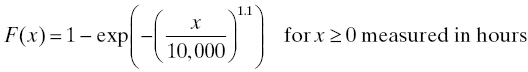
when operated at 20°C. Suppose 100 capacitors from this population are placed into operation (at 20°C) at a time we will designate by 0. After 1000 hours of uninterrupted operation have passed, what is the expectation and standard deviation of the number of capacitors that will still be working?
Solution: The number of capacitors still working at time x has a binomial distribution with parameters 100 (the number of trials in the experiment) and the probability of survival of one capacitor past time x. For x = 1000, this probability is

As the expected value of a binomial random variable with parameters n and p is np, the expected number of capacitors still working after 1000 hours is 100 × 0.92364 = 92.364. The variance of a binomial distribution with parameters n and p is np(1 − p), which in this case is equal to 7.05292. Consequently, the standard deviation of the number of capacitors still working after 1000 hours is equal to 2.65573.
Requirements tip: We have carried out the computations in this example to five decimal places, which is far more than would be desirable in almost any systems engineering application, solely for the purposes of illustrating the computations. Choose the appropriate number of decimal places whenever a quantity is specified in a requirement. The choice is often dictated by economic factors, practicality of measurement factors, and/or commonsensical factors that indicate how many places is too many for the application contemplated. For instance, specifying the length of a football field, in feet, to two decimal places is too much precision, whereas specifying the dimensions (in inches) of a surface-mount component may require more than two decimal places. Note that the units chosen bear on the decision as well.
3.3.2.2 Definition of the survivor function
The example points to another useful quantity in reliability modeling of nonmaintained units, and that is the survivor function or reliability function. The survivor function is simply the probability that a unit chosen at random from the population is still working (“alive”) at time x:
and is consequently one minus the life distribution (the complement of the life distribution) at x. Again, a subscript L is sometimes used if it is necessary to avoid ambiguity.
Note that we have consistently pointed out that the discretionary variable x is nonnegative in lifetime applications. This is because, for obvious physical reasons, a life distribution can have no mass to the left of zero. That is, the probability of a negative lifetime is zero. Lifetimes are always nonnegative, so when L is a lifetime random variable, there is no point in asking for P{L ≤ x} when x < 0 because P{L ≤ x} = 0 whenever x < 0.
3.3.2.3 Properties of the life distribution and survivor function
This discussion leads naturally into a discussion of other useful properties of life distributions. We consider four of these:
- The life distribution is zero for x < 0.
- The life distribution is a nondecreasing function of x for x ≥ 0.
- F(0−) = 0 and F(+∞) = 1.
- The life distribution is continuous from the right and has a limit from the left at every point in [0, ∞).
Return to Figure 3.1 to explore how the generic (continuous) life distribution shown there has these properties. We have indicated in Section 3.3.2.1 how the first property comes about. For the second property, consider that F(x) is the probability that a unit5 fails before time x. That is, F(x) is the probability that the unit fails in the time interval [0, x]. Choose now x1 and x2 with x1 < x2 and consider F(x1) and F(x2). The interval [0, x2] is larger than (and in fact contains) the interval [0, x1], so there are more opportunities for the unit to fail in the additional time from x1 to x2.6 Thus F(x2) must be at least as large as F(x1), which is property 2. From property 3, F(0−) = 0 says that the limit as x → 0 from the left (i.e., through negative values) of the probability that a unit fails immediately upon being placed into operation is zero. F(+∞) = 1 says that every unit in the population eventually fails. There are situations in which we may wish to assume F(0) > 0 (an example is given by a switch that fails to operate when called for) or F(+∞) < 1 (an example could be some component that is certain to not fail until after the service life of the system in which it is used is expired). But in most cases, property 3 is used as stated. Finally, the continuity of the life distribution from the right is a consequence of the choice of ≤, rather than <, in the cdf definition of life distribution. An equally satisfactory probability theory can be constructed on the choice of < (and in fact many notable probability textbooks do this), but the convention we have chosen to follow is as above, and in this case the cdf is continuous from the right (in the other case, it is continuous from the left).
Language (and notation) tip: For most of the life distributions in common use in reliability engineering, it is immaterial whether the < sign or the ≤ sign is chosen, because these life distributions are continuous. However, once the choice is made, it is important to continue the current analysis with the same choice throughout for consistency. This only matters when the life distribution has discontinuities (such as the switch life distribution, used in the example in Section 3.4.5.1, which contains a non-zero turn-on failure probability). Even when all life distributions in a study are continuous and it doesn’t make any difference to the outcome, it is just sloppy practice to switch between < and ≤ arbitrarily. When working with someone else’s analysis, endeavor to determine which choice was made and whether it is consistently applied.
Because the survivor function S is the complement of the life distribution F (i.e., S = 1 − F), the corresponding four properties for the survivor function are
- The survivor function is one for x < 0.
- The survivor function is a nonincreasing function of x for x ≥ 0.
- S(0−) = 1 and S(+∞) = 0.
- The survivor function is continuous from the left and has a limit from the right at each point in [0, ∞).
Language tip: The survivor function is also sometimes called the reliability function. Recalling our discussions from the Foreword and Chapter 2, the fact that we have just encountered yet another use of the same word “reliability” should strengthen your resolve to master potential confusions inherent in this language and be prepared to clarify for your teammates, customers, and managers another of the many unfortunate language clashes that abound in reliability engineering.
3.3.2.4 Interpretation of the life distribution and survivor function
The easiest way to maintain a consistent interpretation of the life distribution and survivor function is to visualize
- the population of components to which they apply and
- the “experiment” of choosing an item from that population at random.7
When you make this choice at a certain time (call it t, meaning that you have chosen some time to start a clock and that clock now measures t time units later), the probability that the item chosen is still alive (“working”) at that time is given by the value of the survivor function S(t) for that population. Because of the nature of selection at random without replacement, the number of items in the population still alive at time t is a random variable having a binomial distribution. If the initial size of the population is A < ∞ and N(t) denotes the (random) number of items still alive at time t, then

This is a binomial distribution with parameters A and S(t). Its mean is AS(t) and its standard deviation is ![]() . So the expected proportion of the population that is still alive at time t is AS(t)/A = S(t). As more time passes (t increases), this proportion does not increase.
. So the expected proportion of the population that is still alive at time t is AS(t)/A = S(t). As more time passes (t increases), this proportion does not increase.
Similarly, the (random) number of items that have failed by time t (or, to put it another way, the number of items that have failed in the time interval [0, t] from 0 to t) has a binomial distribution with parameters A and F(t) = 1 − S(t).
Language tip: Note that we have used t and x interchangeably in this section to denote a discretionary variable having the dimensions of time. This is not cause for alarm. It is routinely acceptable provided the definition is clear and the same letter is used consistently throughout each application.
3.3.3 Other Quantities Related to the Life Distribution and Survivor Function
As with cumulative distribution functions in probability, other related quantities enhance our ability to make reliability models. The ones we shall study in this section are the density and hazard rate.
3.3.3.1 Density
Should it happen that the life distribution is absolutely continuous (i.e., can be written as an indefinite integral of some integrable function), that integrable function is called the density of the lifetime random variable. So if we can write
for some integrable function f, then f is called the density of F. If this is the case, then F is necessarily continuous at every x for which this equation holds. More simply, if F is differentiable on an interval (a, b), then it is absolutely continuous there and f(x) = F΄(x) = dF/dx for x ∈ (a, b). Because of properties 1 and 2 of life distributions, we have f(x) = 0 for x < 0 and f(x) ≥ 0 for x ≥ 0. Most of the life distributions in common use in reliability modeling have densities (see the examples in Section 3.3.4) (Figure 3.2).

Figure 3.2 A generic density function.
Example: Suppose F(t) = t/(1 + t) for t ≥ 0 and F(t) = 0 for t < 0. Then properties 1, 3, and 4 (Section 3.3.2.3) are readily verified. Also, F is differentiable on [0, ∞) and F΄(t) = 1/(1 + t)2 > 0 there, so F is increasing (property 2) and f(t) = 1/(1 + t)2 is its density. Thus, this F is a life distribution with a density.
3.3.3.2 Interpretation of the density
When the lifetime L has a distribution F that has a density in a neighborhood of a point t, we may write
That is, for a small positive increment ε, the probability that an item chosen at random from the population fails in the (small) time interval [t, t + ε] is approximately ε times the value of the density at t. Note that this item may have already failed before time t—there is no requirement that the item be alive at the beginning of this interval. Contrast this with the hazard rate interpretation discussed in Section 3.3.3.5.
3.3.3.3 Return to the stress–strength model
The stress–strength model was introduced in Section 2.2.7 and the example of destruction of a single complementary metal-oxide semiconductor (CMOS) integrated circuit was explained as resulting from a single environmental stress, namely the application of a voltage stress exceeding the strength of the oxide in the device. Here we explore the stress–strength model in a population of devices and an environment that can offer a range of stresses.
Imagine that a population of devices has a range of strengths that is described by a strength density. That is, for some device characteristic V that indicates “strength” (e.g., oxide breakdown voltage), there is a density fV characterizing that population with respect to that strength variable, or characteristic. That means that we describe the strength of an item drawn at random from the population by a random variable V that has density fV, and when that item is subjected to a stress greater than V, it fails. Further suppose that the environment offers stresses (on the same scale) described by a random variable S with density gS. Figure 3.3 shows this relationship graphically. The density of stresses offered by the environment, gS, and the density of strength in the population of devices, fV, is shown on the same axes. Figure 3.3 depicts a situation where most of the population strengths are greater than most of the environmental stresses, except for the small area where the two densities overlap. For a stress in this area (a value indicated by the × on the horizontal axis), a device whose strength is to the left of this stress (weaker than this stress) will fail. In this picture, this small area indicates that there are few devices in the population whose strength is less than (to the left of) this value. The area under the stress density to the right of the chosen stress value is also small, and this indicates that stresses so large are rarely offered (most stresses are less than this value, or almost all of the stress density lies to the left of this value).
Figure 3.3 Stress–strength relationship in a population.
The probability of failure, P{S > V}, is the probability that a stress chosen at random from the population of stresses (described by the density gS) exceeds the strength of a device chosen at random from the population of devices whose strength density is fV. Then the probability of failure of a device drawn at random from that population, when subjected to a stress drawn at random from that environment, is
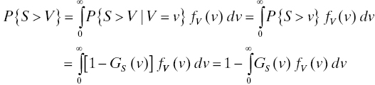
as long as we assume the environmental stresses are stochastically independent of the population strengths.
Note that neither of these relates to time to failure. The distributions (densities) here are both on a scale of some physical property (e.g., volts). To develop this model further to the point where a lifetime distribution could be obtained, it would be necessary to describe the times at which the environment offers stresses of a given size. This could be done with, for example, a compound Poisson process in which at each (random) time an event occurs, a stress of a random magnitude is applied. Some details of this model may be worked out in Exercise . A deeper discussion of stress–strength models is found in Ref. 38.
3.3.3.4 Hazard rate or force of mortality
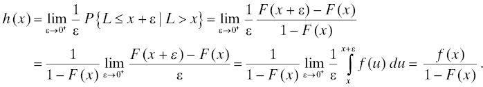
The second related quantity, one that is widely used in modeling the reliability of nonmaintained units, is the hazard rate. The hazard rate is customarily denoted by h, and the definition of hazard rate is

when the limit exists. This is the hazard rate of the lifetime random variable L. It is also sometimes spoken of as the hazard rate of the life distribution. Note this definition contains a conditional probability, and, unlike the quantities we have studied so far which are dimensionless, the hazard rate has the dimensions of 1/time (probability is dimensionless and ε has the dimensions of time).
In case F is absolutely continuous at x, the hazard rate may be computed as follows:
If we further assume F is differentiable, the differential equation
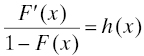
with initial condition F(0) = α may be solved to yield

Thus when the life distribution is differentiable, there is a one-to-one correspondence between the life distribution and its hazard rate. Knowing either one enables you to obtain the other. Most often α will be zero, but it is useful to know the expression for life distribution in terms of hazard rate even when α > 0. An example of a component whose life distribution is a switch for which the probability of failure when it is called upon to operate is α > 0.
3.3.3.5 Interpretation of the hazard rate
Return to the definition above to see that
as ε → 0+. Imagine for the moment that time is measured in seconds and consider this equation for ε = 1 (second). Then the hazard rate at x is approximately equal to the conditional probability of failure in the next second (i.e., before time x + 1) given that the unit is currently alive (using time x to represent the current time). So the hazard rate is something like the propensity to fail soon given that you are currently alive. In fact, the concept of hazard rate is lifted directly from demography, the study of lifetimes of human populations, where it is called the force of mortality. This description is very apt: the hazard rate, or force of mortality, describes how hard nature is pushing you to die (very) soon when you are alive now.
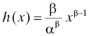
Example: Let F(x) = 1 − exp((−x/α) β) for x ≥ 0 and F(x) = 0 for x < 0, where α and β are positive constants. This is readily verified to be a life distribution (Exercise 2). Its particular properties depend on the choice of the constants α and β which are called parameters. This life distribution is called the Weibull distribution in honor of the Swedish engineer, scientist, and mathematician Ernst Hjalmar Wallodi Weibull (1887–1979). See also Section 3.3.4.3. This distribution has a density
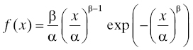
for x ≥ 0. Consequently, the hazard rate of the Weibull distribution is given by
again for x ≥ 0.8 It follows from this expression that the hazard rate of the Weibull distribution may be increasing, decreasing, or constant, depending on the choice of β: if β < 1, the hazard rate is decreasing, if β > 1, the hazard rate is increasing, and if β = 1, the hazard rate is constant. The special case β = 1 has a long and extensive usage in reliability modeling: it is the exponential life distribution F(x) = 1 − exp(−(x/α)) (Section 3.3.4.1). We have seen that the hazard rate of the exponential distribution is constant; it has been shown that this is the only life distribution in continuous time whose hazard rate is constant [34] (the geometric probability mass function p(x) = (1 − α)α x−1 for x = 0, 1, 2, . . . and 0 < α < 1 is a life distribution on a discrete time scale that has a constant hazard rate, and it is the only life distribution in discrete time that is so blessed [35] ). We will explore additional properties of the exponential distribution when we discuss more examples in Section 3.3.4.
Finally, contrast the interpretation of hazard rate with the interpretation of density given in Section 3.3.3.2. Owing to the equation
ε times the density at t is approximately equal to the probability that a lifetime falls between t and t + ε, that is, the probability that L > t and L ≤ t + ε. Here, we are selecting a unit at random from the population and asking if its lifetime is between t and t + ε. The hazard rate, instead, satisfies
which indicates that ε times the hazard rate at time t is approximately equal to the conditional probability that a lifetime expires (at or) before t + ε, given that it is greater than t. Here, we are selecting from a restricted portion of the population, namely that set of units whose lifetimes are greater than t (those that are still alive at time t). Selecting a unit at random from those, we ask what is the probability that the lifetime of that unit does not exceed t + ε. In more mathematical terms, this is the difference between P(A ∩ B) and P(A | B).
Language tip: The hazard rate or force of mortality is almost always called the failure rate of the relevant life distribution. This is unfortunate, the more so because it is almost universal, because the word “rate” makes engineers think of “number per unit time,” and there is nothing like that going on here (even though the dimensions of the hazard rate are 1 over time). The closest one can come to interpreting “hazard rate” as a rate is as in the following example. Suppose the population of units we are considering initially contains N members and we start all of these operating at an arbitrary time we shall label “zero.” At a later time x, the expected number of failed units is NF(x) (where F is the life distribution for this population) and the expected number of units still working is NS(x) = N(1 − F(x)). One of these still-alive units fails before time x + 1 with probability approximately equal to h(x).9 So the hazard rate is like the proportion of the remaining (still-alive) population that is going to fail very soon. This looks like a “rate” when referred to the number of remaining (still-alive or “at-risk”) members of the population. Extended discussion of this deplorable situation is available in Ref. 2. See also the “Language Tips” in Section 4.4.2.
Requirements tip: Be very careful when contemplating writing a requirement for “failure rate.” Because the phrase can be interpreted in (at least three) different ways in reliability engineering, it is vital that you specify which meaning is intended in the requirement. For this reason, it is probably best to avoid “failure rate” altogether in requirements. Instead, spell out the specific reliability effectiveness criterion intended. For example, “The number of system failures shall not exceed 3 in 25 years of operation under the specified conditions” is preferable to “The system failure rate shall not exceed 1.37 × 10⁻⁵ failures per hour during the service life of the system when operated under specified conditions.” Indeed, the latter formulation tends to induce one to think that system failures accrue uniformly over time, while the former formulation allows for arbitrary patterns of failure appearance in time, as long as the total number does not exceed 3 in 25 years.
The concept of cumulative hazard function will be useful later in the study of certain maintained system models (Section 4.4.2). The cumulative hazard function H is simply the integral of the hazard rate over the time scale:
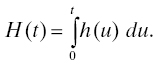
It is easy to see that H(t) can also be written as H(t) = −log S(t) = −log [1 − F(t)].
3.3.4 Some Commonly Used Life Distributions
3.3.4.1 The exponential distribution
The lifetime L has an exponential distribution if P{L ≤ x} = 1 − exp(−x/α) for x ≥ 0 and α > 0. α is called the parameter of the distribution. As x has the dimensions of time, so does α because the exponent must be dimensionless. In fact, α is the mean life:

The exponential distribution has a density, namely (1/α) exp(−x/α). Consequently, the hazard rate of the exponential distribution is constant and is equal to 1/α. Note this has the units of 1 per time as it should. The variance of the exponential distribution is
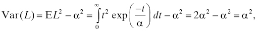
so its standard deviation is α. The median of the exponential distribution is the value m for which P{L ≤ m} = 0.5; solving exp(−m/α) = 0.5 for m yields m = α log 2.
Frequently, the exponential distribution is seen with the parameterization 1 − exp(−λx) for λ > 0. This is perfectly acceptable; simply replace α by 1/λ in all the earlier statements.
The exponential distribution is also blessed with a peculiar property called the memoryless property. As a consequence of the following computation

we see that if an item’s lifetime L has an exponential distribution, then the probability that the item will fail after the passage of a (additional) units of time is the same no matter how old the item is. That is, if the item is currently x time-units old, then the probability of the item’s surviving to time x + a is the same as the probability that a new item survives to time a, regardless what x may be. To get some sense of how peculiar a property this is, consider the purchase of a used flat-screen television. If reliability were your only concern, and the life distribution of the (population of) flat-screen TV(s) were exponential, then you would be willing to pay the same price for a used flat-screen TV of any age as you would for a new one. Of course, there are other factors at play here, and reliability is not your only concern, but the example serves as a caution you should remember when you contemplate using the exponential distribution for the lifetime or a nonrepairable item. The exponential distribution is the only life distribution (in continuous time) that has this property [34].
One reason for the popularity of the exponential distribution in reliability modeling is that it is the limiting life distribution of a series system (Section 3.4.4) of “substantially similar” components [15] . In this context, “substantially similar” has a precise technical meaning which we will defer discussing until Sections 3.4.4.3 and 4.4.5 when a similar result (Grigelionis’s theorem [53] ) will be seen as relevant to both maintained and nonmaintained systems. Implications for field reliability data collection and analysis are discussed in Chapter 5.
3.3.4.2 The uniform distribution
A random variable L is said to have a uniform distribution on [a, b], a < b, if
If a ≥ 0, the uniform distribution can be used as a life distribution. In this model, the lifetimes are between a and b with probability 1, and the distribution has the name “uniform” because the probability that a lifetime lies within any subset of [a, b] of total measure τ, say, is τ/(b − a) regardless where within [a, b] this subset may lie (as long as it lies wholly within [a, b]). The density of the uniform distribution is 1/(b − a) on [a, b] and zero elsewhere. The expected value of a uniformly distributed lifetime is (a + b)/2 and the variance is (b − a)2/12. In other uses of the uniform distribution, a may be negative, but for use as a life distribution a must be nonnegative. See Exercise 6 for the hazard rate of the uniform distribution.
3.3.4.3 The Weibull distribution
The lifetime L has a Weibull distribution if P{L ≤ x} = 1 − exp(−(x/α) β) for x ≥ 0 and α > 0, β > 0. α and β are the parameters of the distribution. As we saw in the example in Section 3.3.3.4, the Weibull distribution has a density

and its hazard rate is

all for x ≥ 0.
As noted previously, the hazard rate for the Weibull distribution can be increasing, decreasing, or constant, depending on the value of β (Table 3.1).
Table 3.1 Weibull Distribution Hazard Rate
| If β is | Then the Weibull hazard rate is |
| >1 | Increasing |
| =1 | Constant |
| <1 | Decreasing |
When β = 1, the Weibull distribution reduces to the exponential distribution (Section 3.3.4.1). The Weibull distribution with β > 1 is frequently used to describe the lifetimes in a population of items that may suffer mechanical wear. For example, ball bearings normally exhibit wear (decrease of diameter) as they continue to operate.10 A population of identically sized ball bearings made of the same material, when operated continuously, will accumulate more and more failures due to wear as time increases. That is, failures will begin to accumulate more rapidly the longer the population continues in operation. This phenomenon is labeled “wearout” in reliability engineering, the term being inspired by the concept of mechanical wear such as illustrated in this example. Note that this example treats a nonrepairable item. Any individual ball bearing may suffer at most one failure; the “accumulation of failures” pertains to multiple failures in a population of many bearings, each of which may fail at most once. See Section 3.3.4.8 for additional development of this idea.
Finally, the Weibull distribution is the limiting distribution of the smallest extreme value (i.e., the minimum) of a set of independent, identically distributed random variables [27] . The lifetime of a component under the competing risk model (Section 2.2.8) is a smallest extreme value. This may account for the frequent appearance of the Weibull distribution as a reasonable description of the lifetime of individual components.
3.3.4.4 a life distribution with a “bathtub-shaped” hazard rate
Demographers have determined that the force of mortality in human populations follows a broad U-shaped, or “bathtub-shaped,” curve (see Figure 3.4).

Figure 3.4 Force of mortality for human populations.
The commonly accepted explanation for this shape posits that the decreasing force of mortality in early life comes from infant mortality and the diseases that afflict the young, which, after some period of time, are outgrown and subsequently exert little influence on the population. The increasing force of mortality in late life is due in large part to the finite lifetime of human beings (see Exercise 6), but is also due to what are termed “wearout mechanisms” such as atherosclerosis, loss of telomeres, and others, that promote earlier death. The (approximately) constant force of mortality in mid-life is primarily due to deaths caused by accidents that occur at random times and the rarer occurrence of diseases that strike prematurely in middle age. A similar interpretation obtains in reliability engineering: decreasing force of mortality in the early part of the lifetime in a population of components is explained by the early failure of some components in the population that have manufacturing defects (see Section 3.3.6) that cause them to fail prematurely (such failures are often referred to as “infant mortality failures”). Increasing force of mortality in the later part of the lifetimes is explained by physical and chemical wearout mechanisms such as mechanical wear, depletion of reactants, increase of nonradiative recombinations, increase in the number and/or size of oxide pinholes, etc. Indeed, the presence of an increasing hazard rate is often taken as a symptom of the presence of an active wearout failure mode, even if no physical, chemical, or mechanical wearout explanation can be discerned. The constant force of mortality during “useful life” is due primarily to the occurrence at random times of shocks whose stresses exceed the strengths of the components (see Section 3.3.3.3 and Exercise 1).
None of the life distributions discussed elsewhere in this section has a force of mortality with this shape. To develop such a life distribution, we need to employ the method shown in Section 3.3.3.4 in which a life distribution is developed from a hazard rate by the integral formula shown there.
At least one attempt at implementing a practical version of such a life distribution has been made. Holcomb and North [30] introduced a life distribution of this type for electronic components. Their model is a Weibull distribution describing the component’s reliability until a time called the crossover time, at which time it changes to an exponential distribution that applies thereafter. That is, the population life distribution is described by a Weibull distribution up until the crossover time, and the (conditional) life distribution of the subset of the population that survives beyond the crossover time is an exponential distribution. This distribution is continuous everywhere and has a density everywhere except at tc. The hazard rate model is as follows:
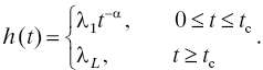
This model contains four parameters, λ1, λL, tc, and α. λ1 > 0 is the early life hazard rate coefficient and represents the hazard rate of the life distribution at t = 1 (conventionally, the time unit in this model is hours). α > 0 is the early life hazard rate shape parameter; it represents the rate at which the hazard rate decreases until time tc. At time tc, the hazard rate becomes equal to a constant λL > 0. The model further imposes the condition that the hazard rate be continuous, so the four parameters are not independent. They are linked by the relation
Note that while this hazard rate model allows for a decreasing hazard rate in early life and a constant hazard rate in “mid-life,” the increasing hazard rate characteristic of wearout is not present. This is because it was reasoned that wearout mechanisms in electronic components take so long to appear that the service life of the equipment or system is over before this occurs.11 Finally, note that in this model the conditional life distribution of components, given that they survive beyond tc, is exponential with parameter 1/λL.
For the life distribution and density corresponding to this hazard rate model, see Exercise 7.
3.3.4.5 the normal (Gaussian) distribution: a special case
A random variable Z has a standard normal (or standard Gaussian) distribution if
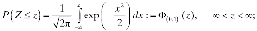
the mean of this distribution is 0 and its variance is 1 (this is the definition of “standard” for the normal distribution and the explanation of the subscript on the Φ). The density of this distribution is given by

Clearly, evaluating the normal distribution is not a paper-and-pencil exercise. The old-school method is to use the table of standard normal percentiles, which appears in all elementary statistics textbooks; the tables are usually constructed by numerical integration or polynomial approximation [1] . Now, all statistical software and many scientific calculators include a routine for evaluating the standard normal distribution, and many office software programs, such as Microsoft Excel®, also include this capability.
If Z is a standard normal random variable, the random variable σZ + μ has mean μ and variance σ2 where −∞ < μ < ∞ (could be negative!) and σ > 0; the distribution of σZ + μ is conventionally denoted by Φ(μ,σ) or simply Φ if μ and σ are clear from the context. Correspondingly, if Z is a normally distributed random variable having mean μ and standard deviation σ, then (Z − μ)/σ has a standard normal distribution. The normal distribution is also called the Gaussian distribution in honor of the great mathematician Carl Friedrich Gauss (1777–1855) who first used it to describe the distribution of errors in statistical observations.
The normal distribution is not a life distribution because it has mass to the left of 0, i.e., it gives positive probability to negative lifetimes. Nonetheless, some studies use a normal distribution with large positive μ and small σ as an approximate life distribution because when μ is large positive and σ is small, the probability that the lifetime is negative is quite small and may for some purposes (e.g., computing moments) be neglected. However, the normal distribution is not appropriate for use with many of the important models for the reliability of a maintainable system. For example, the equations of renewal theory (Section 4.4.1) fail for the normal distribution (even if μ is large positive and σ is small).
Some studies make use of a truncated normal distribution to avoid the difficulty with negative lifetimes. A truncation of a normal distribution with parameters μ and σ is the conditional distribution of a random variable Y that is normally distributed with mean μ and variance σ2, conditional on Y belonging to some interval. To use the truncated normal distribution as a life distribution, this interval would be [0, ∞], or the conditioning is on Y ≥ 0. If we denote by W the lifetime random variable described by this truncated distribution, then
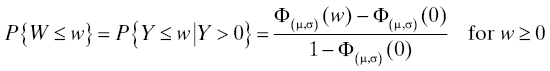
and P{W ≤ w} = 0 for w ≤ 0 so that the truncated normal distribution is a bona fide life distribution. Note that the mean and variance of the truncated normal distribution are no longer μ and σ2. For more details on the truncated normal distribution, see Ref. 28.
3.3.4.6 the lognormal distribution
A lifetime L is said to have a lognormal distribution if the logarithm of the lifetime has a normal distribution. That is,
Note that while L ≥ 0, log L may have any sign because the logarithms of numbers between 0 and 1 are negative. If Y has a normal distribution, then L = eY has a lognormal distribution. If μ and σ are the parameters of the underlying normal distribution, then the mean of the lognormal distribution is ![]() and its variance is
and its variance is ![]() .
.
The lognormal distribution has been successfully used for modeling repair times of complex equipment [37, 51]. Its hazard rate is decreasing as t → ∞, leading to the interpretation that when equipment is complex, repairs are often complicated, and the longer a repair lasts, the less likely that it is that it will be completed soon. For example, times to complete repairs for undersea telecommunications cables that require a repair ship to visit the site of the failure have been postulated to follow a lognormal distribution, but citations in the literature are hard to find.12
3.3.4.7 The gamma distribution
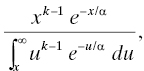
The lifetime L has a gamma distribution if
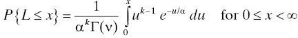
where α > 0 and k > 0 are the location and shape parameters, respectively, of the distribution, and Γ is the famous gamma function of Euler (Leonhard Euler, 1707–1783), defined by
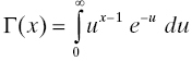
for x > 0. The gamma function is perhaps most well-known for being an analytic function that interpolates the factorial function: Γ(n + 1) = n! whenever n is a positive integer. α is a location parameter and k is a shape parameter (α has the units of time and k is dimensionless); when k = 1 the gamma distribution reduces to the exponential distribution (Section 3.3.4.1) with parameter α. The importance of the gamma distribution in reliability modeling lies largely in its property that the gamma distribution with parameters α and n (n an integer) is the distribution13 of the sum of n independent exponential random variables, each of which has mean α. Actually, more is true: the sum of two independent gamma-distributed random variables with parameters (α1, ν) and (α2, ν) again has a gamma distribution with parameters (α1 + α2, ν), and of course this extends to any finite number of summands as long as the shape parameter ν is the same in each. There is a natural connection with the life distribution of a cold-standby redundant system (see Section 3.4.5.2 for further details).
The density of the gamma distribution is given by

Consequently, the hazard rate of the gamma distribution is given by
again for x > 0. When k = 1, this reduces to 1/α, a constant, as it should because for k = 1 the gamma distribution is the exponential distribution. The hazard rate is clearly increasing for k > 1; it is the content of Exercise 3 that the hazard rate is decreasing when 0 < k < 1. So the behavior of the gamma distribution is similar to that of the Weibull distribution according to the shape parameters (Table 3.2).
Table 3.2 Gamma Distribution Hazard Rate
| If k is | Then the gamma hazard rate is |
| >1 | Increasing |
| =1 | Constant |
| <1 | Decreasing |
The mean of the gamma distribution is kα and its variance is kα2.
The main importance of the gamma distribution elsewhere comes from its relation to commonly used quantities in statistics that we use in Chapters 2, 5, 10, and 12. The sample variance from a population having a normal distribution has a gamma distribution. Formally, if X1, X2, . . ., Xn are normally distributed random variables with mean 0 and variance σ2, then X1 2 + X2 2 + ⋅ ⋅ ⋅ + Xn 2 has a gamma distribution with parameters 1/2σ2 and n/2. For historical reasons, this distribution when σ = 1 is also called the chi-squared distribution with n degrees of freedom (Karl Pearson, 1857–1936). Other important quantities in statistics have distributions related to the gamma distribution, including student’s T-statistic (student was a pseudonym adopted by William Sealy Gosset (1876–1937) to enable him to publish his works over the objections of his employer, the Guinness brewing company), Snedecor’s F-statistic (George W. Snedecor, 1871–1974), and Fisher’s Z-statistic (Sir Ronald A. Fisher, 1890–1962) all have distributions than can be expressed in terms of the gamma function and distribution. For details, see Ref. 21.
3.3.4.8 mechanical wearout and statistical wearout
“Wearout” is used in two senses in reliability engineering. Mechanical wearout is the physical phenomenon of loss of material during sliding, rolling, or other motion of materials against one another. Statistical wearout is the mathematical property of increasing hazard rate of a life distribution when the hazard rate does not decrease after the period of increase being described. The second interpretation arose because of the first: a population of devices subject to (physical) wearout will exhibit a life distribution with an increasing hazard rate in later life. The following example may help illustrate this phenomenon.
Example: A population of 5/8″ ball bearings is operated under nominal conditions under which their diameter decreases by X ten-thousandths of an inch per hour, where X is a random variable having a uniform distribution on [1, 4] (see Section 3.3.4.2). A ball bearing is declared failed when its diameter has decreased by 0.010″. What is the distribution of lifetimes L in this population of ball bearings? For a ball bearing that we label ω, the rate of decrease of its diameter is X(ω), and the amount of time (in hours) it takes for that ball bearing to decrease by 0.010″, which is 100 ten-thousandths, is 100/X(ω) hours. Our task, then, is to find the distribution of 100/X when X has the stated uniform distribution. We know that
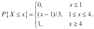
Then
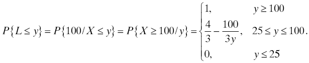
The density of this distribution is 100/3y 2 for 25 ≤ y ≤ 100, and zero elsewhere. So the hazard rate of this distribution is 100/y(100 − y) for 25 ≤ y ≤ 100, and zero elsewhere. This is clearly seen to be an increasing function of y as y → 100− (i.e., as y approaches 100 from the left, or through smaller values, which is what the superscripted minus sign is supposed to convey). This example, while not generic, does illustrate the connection between physical wearout and the mathematical interpretation of wearout as an increasing hazard rate with increasing time. See also Exercises 6, 20, and . Further discussion may be found in Ref. 24.
Another way to understand this phenomenon is to imagine that all the ball bearings wear at exactly the same (constant) rate, say 2.5 ten-thousandths of an inch per hour. Then every ball bearing fails at 40 hours exactly. Then a small variation in the rate of wear (i.e., 0.00025″/hour ± a little bit) will translate into some variation in the failure times (40 hours ± a little bit14). The failure time density will be zero until shortly before 40 hours (i.e., up until 40 – the little bit) and then it will increase rapidly to a maximum near 40 hours and then decrease again rapidly to zero (at 40 + the little bit). The survivor function of the lifetimes will be zero until shortly before 40 hours, and then will decrease rapidly to zero shortly after 40 hours. Think about the quotient of these two quantities (the hazard rate): from shortly before 40 hours until at least 40 hours, the numerator is increasing rapidly while the denominator is decreasing. The quotient is therefore increasing, at least until the density peaks. Deeper analysis would reveal that the hazard rate continues to increase until “shortly after 40 hours,” but that is not the point of this illustration. The point is that under very general conditions, physical wearout, even at random rates, leads to an increasing hazard rate life distribution, which is the characteristic of wearout in the statistical (or mathematical) sense.
3.3.5 Quantitative Incorporation of Environmental Stresses
In Chapter 2, we emphasized that three things must be present in a proper reliability requirement: a specification of a limit on some reliability effectiveness criterion, a time during which the requirement is to apply, and conditions (environmental or other) under which the requirement is to apply. In the discussion of earlier life distributions, no mention is made of conditions. In this section, we will discuss some modifications that enable us to incorporate the role of prevailing conditions into a life distribution model.
3.3.5.1 accelerated life models
Accelerated life models are among the simplest models for relating the life distribution of a population of objects operated under a given set of environmental conditions to the life distribution of that population operated under a different set of environmental conditions. We describe two accelerated life models in this book, the strong accelerated life model and the weak accelerated life model, and the proportional hazards model which in analogous terminology might be called the accelerated hazard model.
The strong accelerated life model postulates that there is a linear relationship between the individual lifetimes at the different conditions. If L1 and L2 are the lifetimes of an object when the conditions under which it is operated are C1 and C2, respectively, then the strong accelerated life model asserts that L2 = A(C1, C2)L1, where A is a constant depending on the two conditions C1 and C2.15 If many conditions change from one application to another, it is possible that C1 and C2 may be vectors. If the conditions are dynamic (may change with time), then C1 and C2 may be functions of time.
We begin our study with the simplest case in which the two conditions are constant. For example, condition C1 may be a constant temperature of 10°C, while condition C2 may be a constant temperature of 40°C. Typically, one of these conditions, say C1, represents a “nominal” operating condition, that is, a condition under which life distribution estimates for the population are known (or the conditions prevailing when the data for these estimates were collected), and the other condition C2 represents a condition under which operation of the system is anticipated in service with the customer. The types of environmental conditions that are typically encountered in engineering systems include
- temperature,
- humidity,
- vibration,
- shock, and
- mechanical load.
This list is far from all-inclusive. It includes only those conditions that are commonly encountered. Other more specialized conditions may include salt spray and immersion for marine environments, dust and oil spray for automotive environments, etc.
If a population follows the strong accelerated life model, the life distributions at the different environmental conditions differ only by a scale factor. In fact we have, for F1 the life distribution of L1 and F2 that of L2,
showing that the scale factor is 1/A(C1, C2). For the densities, we have
and for the hazard rates, we have
Example: Suppose that, under nominal conditions, a population of devices has a Weibull life distribution with parameters α = 20,000 and β = 1.4 (see Section 3.3.4.3). Under the strong accelerated life model, what are the new parameters of the life distribution when the population is operated at conditions for which the acceleration factor is 8? Denote by the subscript 1 the nominal conditions and by the subscript 2 the operating conditions (for which the acceleration factor is 8). Then

so the life distribution parameters under the operating conditions are α = 160,000 and β = 1.4.
From the example, we may gather that if the life distribution at nominal conditions has a certain parametric form, then the life distribution at any altered conditions continues to have the same parametric form when the strong accelerated life model applies (see Exercise 8).
We summarize the strong accelerated life model in Table 3.3.
Table 3.3 Strong Accelerated Life Model
| Description | Formula |
| Lifetime (or failure time) | L2 = A(C1, C2)L1 |
| Life distribution | F2(t) = F1(t/A(C1, C2)) |
| Density | f2(t) = f1(t/A(C1, C2))/A(C1, C2) |
| Hazard rate | h2(t) = h1(t/A(C1, C2))/A(C1, C2) |
In the strong accelerated life model, the defining equation L2 = A(C1, C2)L1 shows that the individual lifetimes under the two conditions are proportional. In fact, the probabilist would write L2(ω) = A(C1, C2)L1(ω) to emphasize that the proportional relationship holds for each individual lifetime (sample point ω in the sample space, or individual member of the population). This is a very strong assumption, but one that is in very common use. Weaker versions of the accelerated life model are available. One such is the weak accelerated life model that postulates the life distribution relationship F2(t) = F1(t/A(C1, C2)) without the assumption that the lifetimes are proportional as individuals. For this weaker model, all the relationships in Table 3.3 apply except for that in the first row. In practice, usually the weak accelerated life model is all that is needed to make sensible use of the accelerated life model ideas.
Requirements tip: In a reliability requirement, while you do specify the environmental conditions that will prevail during operation with the customer and under which the specified reliability is to be achieved, the model to be used when projecting reliability under the operating conditions when the base reliability estimates pertain under some other, “nominal,” conditions is not normally part of the requirement. The choice of model to use when projecting potential system life distributions or when analyzing field reliability data would normally be made by a reliability engineer who is familiar with the system, its components, and the operating environment(s). Systems engineers, while not necessarily themselves carrying out the computations involved, need to be aware of the options available and be able to ascertain whether the reliability engineer’s choice is suitable given all the conditions prevailing.
How do you tell whether an accelerated life model is appropriate? If you have lifetime data collected under two different operating conditions, then the strong accelerated life assumption is easily tested. From the defining equation of the strong accelerated life model, we have
Therefore, if the strong accelerated life model applies, a quantile–quantile plot (Q–Q plot) [45] of the logarithms of the lifetimes should have slope 1 and vertical intercept log A. The Q–Q plot is a graphical aid for determining when the strong accelerated life model might be appropriate and provides a method for an initial guess at the value of A.
The foregoing development leaves open the structure of the function A. In practice, different functions A are associated with different types of stresses (temperature, voltage, vibration, etc.). One of the most commonly used in reliability modeling is the Arrhenius relationship (Svante August Arrhenius, 1859–1927) for temperature:
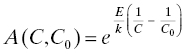
where C and C0 represent the two temperatures in °K (Kelvins), E is an activation energy in electron-volts (eV) particular to the material, and k is Boltzmann’s constant 8.62 × 10⁻⁵ eV/°K. This equation was first used to describe the speeding up of chemical reactions when heat is added and has been widely used in reliability engineering as an empirical acceleration factor, even for phenomena that do not involve heat.
Example: Suppose that, when operated at 10°C, a population of devices has a Weibull life distribution with parameters α = 20,000 and β = 1.4 (see Section 3.3.4.3). Under the strong accelerated life model, what are the new parameters of the life distribution when the population is operated at 35°C? Assume the weak accelerated life model and that the Arrhenius relation holds for these devices with an activation energy of 1.2 eV.
Solution: The Kelvin temperatures corresponding to 10 and 35°C are 283.15 and 308.15, respectively. Then the acceleration factor is
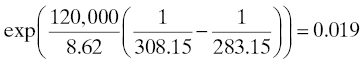
so the life distribution of the population at 35°C is
Many other parametric acceleration functions are used for stress modeling. These include
- the Eyring equation
 , with the single parameter β, is used for temperature, humidity, and other stresses [16] ;
 - the inverse power law model
 , with the single parameter n, is usually used for voltage [16] ; and
 - the Coffin–Manson equation [18], similar to the inverse power law model, used for modeling fatigue under thermal cycling and modeling solder joint reliability.
Environmental conditions in operation may also vary with time. In this case, C1 and C2 may be functions of time. Generalizations of the accelerated life model can be devised to cover this case. One such generalization is a differential accelerated life model. This model postulates that the differential change in the lifetime of a unit is proportional to the current value of stress on the unit. Begin with the equation for the strong accelerated life model:
and include the time dependence of C:
If the life distribution in the population at condition C0 is F0, then the population life distribution after t time units has passed is

(see Section 6.4.3 of [41]). This model is used in analysis of data from accelerated life tests that use time-varying stresses such as ramp stress in which the stress takes the form C(t) = a + bt.
Many other models exist for relating the life distribution of a population operated at some set of environmental conditions to the life distribution of the same population operated at a different set of environmental conditions. Perhaps the most flexible of these is the acceleration transform developed by LuValle et al. [42] . See also Refs. 20, 43.
3.3.5.2 the proportional hazards model
The proportional hazards model is similar to the accelerated life model in that it postulates that certain quantities are proportional: in this case, it is the hazard rates, not the lifetimes, that are proportional. That is, the model postulates that
where h1(t) (resp., h2(t)) denotes the hazard rate of the population when the conditions under which the population is operated are described by C1 (resp., C2). Note the difference with the accelerated life model (Table 4.1). The proportional hazards model was first described by Cox [13] and is widely used in biomedical studies. h1(t) is referred to as the “baseline hazard rate” and is usually associated with a nominal set of conditions such as the conditions under which the data characterizing the population were collected (i.e., the same idea as seen in the accelerated life model, Section 3.3.5.1). See Exercise 22.
3.3.6 Quantitative Incorporation of Manufacturing Process Quality
A commonly accepted explanation for so-called early life failures is that the population contains items that have manufacturing defects (see Section 3.3.4.4). In other words, components or subassemblies used in the system are received from their manufacturer(s) with defects that are undetected and not remedied by the manufacturers’ process controls. The model is that such a defect will activate, or “fire,” at some later time and cause a failure at that time. Using this reasoning, one may seek to construct a model for the early-life reliability of a component or subsystem that contains some factor related to the manufacturer’s process quality. This model may also be used for the whole system to describe the influence of manufacturing processes on its reliability although the generally larger number of manufacturing processes involved may make the model more complicated. One attempt at creating such a model is described in Ref. 56 . A brief summary is given in this section.
We may think of manufacturing as an opportunity to add defects to a product in the sense that when a product (here interpreted broadly to include components, subassemblies, and entire systems) is designed, it has a certain reliability that is a consequence of the degree to which design for reliability (Chapter 6) for the product is successful. The reliability of any realization of this design in physical space can never be better than this because additional failure modes are introduced by this realization, some failure modes were not anticipated in the design for reliability process, etc. The approach taken in Ref. 56 to model this situation is to allow the life distribution for a product to depend also on a parameter that represents the quality of the manufacturing process for that product.
Suppose the lower and upper specification limits for the product’s manufacturing process16 are aL and aU, respectively, and aL < aU. The center of the process’s specification window is a 0 = (aL + aU)/2, which we also assume to be the target of the process output. Finally, we postulate that the true process output is a random variable A that is normally distributed with mean μ and variance σ2 (see Figure 3.5). The process meets “six sigma” goals [29] if there is an m, 4.5 ≤ m ≤ 7.5, for which

Figure 3.5 Specification limits and process output.
If m = 6, the process is centered and the expected fraction of defective process outputs (those falling outside the specification window) is approximately 9.87 × 10⁻¹⁰, or about one part per billion (PPB). The expected fraction of defective outputs is largest when the process center is as far away from a 0 as possible. The maximum deviation allowed by the six-sigma methodology is 1.5 standard deviations, corresponding to m = 4.5 (left of center) or m = 7.5 (right of center). At the maximum deviation, the expected fraction of defective process outputs is approximately 3.4 × 10⁻⁶, or about 3.4 parts per million (PPM).
To incorporate this understanding into a reliability model for the product, we postulate that when the process output is a, a defect may be introduced into the product that causes a failure at a later (random) time X(a). Denote by F(x, a) the life distribution of the failure mode attributable to this defect. That is,
Then the distribution of the time at which the product fails (from this failure mode) is

To make progress, we need to make some assumption about how F(x, a) depends on a. For now, it is reasonable to assume that the further a process output is away from the process center, the more likely it is that the firing time of the associated defect is smaller. Formally, this is expressed as F(x, a) ≤ F(x, a′) whenever |a − a 0| ≤ |a′ − a 0|, or X(a) is stochastically larger [52] than X(a′) whenever |a − a 0| ≤ |a′ − a 0|.
Suppose now that there are M ≥ 1 downstream manufacturing and other product realization processes for this product, and that process j has lower and upper specification limits aj L and aj U, respectively, center aj 0, and output Aj whose mean and standard deviation are μj* and σj, respectively, for j = 1, . . ., M. As is customary in quality engineering studies, we assume all process outputs are normally distributed. The time at which an item chosen at random from this population of products fails is
which, if the firing times are stochastically independent, has the survivor function
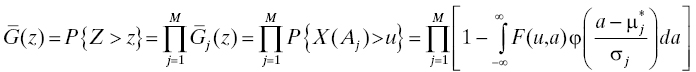
where φ represents the standard normal density.
It follows that
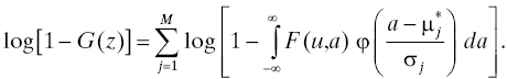
Using the result of Exercise 24 with ![]() you can show that
you can show that
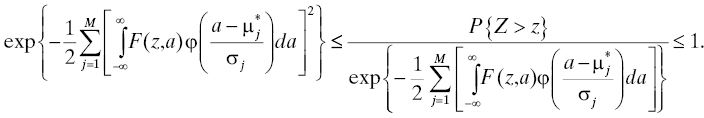
Multiplying everything by the denominator in the middle term gives lower and upper bounds for the survivor function of the product (considering these failure modes only).
3.3.7 Operational Time and Calendar Time
Throughout this section, the functions we use to describe reliability all use “time” as the argument. When so used, “time” almost always means operational time, or the amount of time the system is on and in use. Cumulative operational time does not increase when the system is off and not in use. When writing a reliability requirement, the “time” component of the requirement is intended to capture any increase in age of the system, where “age” refers to progression of any clock measuring time to failure of the system. Usually, this is operational time, so when you need to see how the requirement plays out in calendar time (e.g., warranties are usually written in terms of calendar time), it is necessary to understand the relationship between operational time and calendar time. This comes from how the customer uses the system. Some systems, like servers, broadcast transmitters, air traffic control radars, and the like, are intended to be used continuously and for such systems, operational time and calendar time are equal. Other systems, like refrigerators, do not run continuously and accrue age only when running (e.g., only when the compressor is running), so that operational time is less than calendar time for such systems. If there is a known relationship between operational time and calendar time, for example, as a function ξ(t) giving elapsed calendar time ξ required to accrue an amount of operational time t, then the functions describing reliability can be transferred from one to the other using this relationship. This function is nondecreasing, satisfies ξ(t) ≥ t, and may be deterministic or random. For example, if the refrigerator’s compressor runs only 8 hours a day, then the relationship between operational time t and calendar time s for that refrigerator may be described by s = ξ(t) = 3t when t is measured in hours.
The phrase “duty cycle” is also used to describe the fraction of (calendar) time that the system is in use. In the refrigerator example, the duty cycle is 1/3 or 33%.
If L is a lifetime random variable whose distribution in terms of operational time t is known, that is, P{L ≤ t} = F(t), say, then its distribution relative to calendar time s is given by P{L ≤ s} = P{L ≤ ξ(t)} = F(ξ(t)) where t is any value satisfying ξ(t) = s. For instance, if the refrigerator lifetime R has a distribution given by
in terms of operational time t in hours, then the probability that the refrigerator fails before s calendar hours is given by
because, for this refrigerator, s = 3t.
Some systems may accrue age on some other clock besides the operational time or calendar time clocks. That is, progression to failure may be stimulated by some other mechanism in addition to time. A very common example is the automobile, in which age is measured not only by time but also by mileage. An electromechanical relay ages by number of operations in addition to time. Another way to look at this is to consider the system as having two failure mechanisms, one stimulated by the passage of time, and the other stimulated by a second “clock” like number of operations, mileage, etc.17 Let L1 and L2 represent the lifetimes measured in terms of the first and second clocks, respectively, and let s and t denote the first and second clocks. Then the time at which the object fails is min{L1, L2}.
3.3.8 Summary
Section 3.3 has presented several diverse ways of describing the reliability of a nonmaintained system in quantitative terms: the lifetime, life distribution, density, and hazard rate. Most often, reliability engineers will use the hazard rate (force of mortality) as their preferred descriptor, and it will be called by them (almost universally, and inappropriately), “failure rate.” It is vitally important to remember that when dealing with nonrepairable or nonmaintainable items, the use of the phrase “failure rate” should not lead you to think of the possibility of repeated failures of the same item (i.e., failures per unit time); only the most pernicious confusion will arise. It is best (although not yet common practice) to reserve “hazard rate” or “force of mortality” for this concept so that no confusion may arise.
The life distribution of a component may be altered if the component is exposed to environmental conditions other than those under which the data to estimate that life distribution were collected. Section 3.3.5 also discusses three forms of the accelerated life model that can be used to quantitatively describe such alterations. We also refer to the notion of acceleration transform that is a more general approach to this task.
When an explicit understanding of how manufacturing process(es) influence product reliability is needed, Section 3.3.6 provides a model connecting product reliability to the quality of the manufacturing processes for that product. This model provides a quantitative explanation of the phenomenon of “early-life” failures that are postulated to stem from latent defects introduced into the product by manufacturing process outputs that fall outside the process specification limits. More detailed models of this type can be constructed to capture the effects of more specific knowledge about downstream product realization processes.
Finally, we observe that the reliability descriptions that we introduce in this chapter are functions of operating time. When it is important to know how these are related to calendar time, we provide a means for moving easily from an operating time description to a calendar time description and back. We also discuss how this is related to the competing risk model (Section 3.4.4.2).
3.4 ENSEMBLES OF NONMAINTAINED COMPONENTS
3.4.1 System Functional Decomposition
3.4.1.1 system functional decomposition for tangible products and systems
Most often, nonmaintained items are not operated as individuals in isolation. There are exceptions, of course (the famous light bulb being a notable one), but real engineering systems almost always comprise many nonmaintained items and (possibly) maintained items and subassemblies operating together to perform the functions required of the system. So we would like to know how the lifetimes of such ensembles of nonmaintained items are related to the lifetimes of the individual items themselves. The system functional decomposition is a systematic description of how individual components and subassemblies operate together to enable the system to perform its required functions. There is a functional decomposition for every system requirement (of course it is possible that the same functional decomposition may apply to more than one requirement). The system functional decomposition is carried out to a level of detail necessary for which the life distributions of the components or subassemblies in the last layer of the decomposition are known or can be estimated. Before proceeding to the calculus of system reliability, that is, the methods for calculating the life distributions of higher level assemblies from their constituent components, we look at a few examples of system functional decompositions.
3.4.1.2 functional decomposition for services
The services share of the world economy is large and growing. Our study of systems engineering for sustainability includes reliability, maintainability, and supportability of services. Services as understood here include not only the activities traditionally understood as “services” such as telecom services, auto repair service, fuel delivery service, and the like but also the emerging category of computer-based services such as personal computer and smartphone applications, cloud computing services, etc. All of these have the properties that they are intangible and do not exist outside the context of transactions taking place between users and service providers. The key to successful sustainability engineering for services is the realization that all such services are provided by elements of some tangible infrastructure of systems and humans that have to operate together in specified ways to deliver a transaction in the service.
Consequently, the functional decomposition required for reliability engineering for services requires peeling back an additional layer. To properly understand service reliability requires adopting the perspective of the user of the service, and the service functional decomposition consists of a detailed step-by-step description of how the service is provided. That is, a service functional decomposition acts as a bridge between the infrastructure the service provider uses to deliver the service and the user’s understanding of the parts of a service transaction. Then with each step is associated the part(s) of the service delivery infrastructure that are involved in successful completion of that step. In this way, the reliability of the service (service accessibility, service continuity, and service release) [57] is expressed in terms of the reliability characteristics of those infrastructure components [58].
3.4.2 Some Examples of System and Service Functional Decompositions
3.4.2.1 an automobile drivetrain
The drivetrain in an automobile consists of those components that are required for the automobile to move forward. At a level of detail appropriate for this example, we may list these components as the engine, transmission, driveshaft, differential, and the four wheels18 (a wheel comprises a rim and a tire). Each component listed is required for forward motion. If any component ceases to function, then the auto cannot be driven (for the purposes of this simple example, we are ignoring the possibility of partial failures such as loss of a single gear in the transmission) because one of the requirements of the auto is that be able to drive forward. Each component is a “single point of failure” in the sense that if it fails, then the system fails. Systems of this type are discussed in Section 3.4.4.
This example offers further instructional value. Most autos also carry a spare wheel so that if one of the active wheels fails (usually from a tire puncture), the wheel may be removed and replaced by the spare. This is an example of a system with “built-in redundancy.” Redundancy means that there are additional components or subsystems built into the system that may be called on to restore the system to functioning condition when some component of the system fails (of course, the redundant component must be of the same type as the component that failed). In this example, the spare wheel assembly is a “cold standby” redundant unit. This terminology arises from the idea that the spare unit does not operate and accumulate age until it begins service. Systems containing redundant units are discussed in Section 3.4.5.
3.4.2.2 A telecommunications circuit switch
Automatic circuit switching has a long history in the telecommunications industry, starting with the panel office of the 1920s through the step-by-step, crossbar, and stored-program-control electronic systems that were the last generation of circuit switches. Many electronic switching systems were designed for high reliability by being “fully duplicated.” That is, the system comprised two separate, identical call processing units that operated together. Every incoming call was handled by both processing units and sent on to its next destination. The idea was that should one of the call processing units suffer a failure, the other was operating right alongside it and would successfully route the call regardless. This is an example of a “hot standby” redundant system in which the standby or redundant unit(s) are operating (and aging) all the while the main or primary unit is providing service. Within each call processing unit, there are many line-replaceable units that are single points of failure for that individual call processing unit (but not for the system as a whole). This architecture, while costly, enabled extremely high availability: the availability objective for such systems in Bell System service was availability should be greater than 0.9999943, equivalent to an expected outage time of no more than 2 hours in 40 years of operation. See again Section 3.4.5 for discussion of redundant systems.
3.4.2.3 Voice over IP service using a session initiation protocol server
Here is an example of a functional decomposition for a service. Voice over Internet Protocol (VoIP) service is an example of a voice telecom service carried on a packet network. Session initiation protocol (SIP) is one of the ways of setting up VoIP calls from one user to another. There are several different SIP implementations, but all SIP VoIP call setups involve interaction between the user (a “user agent client” (UAC) which is the user’s local VoIP phone or computer) and a server (“user agent server” (UAS) which is part of the service provider’s infrastructure). To successfully set up and carry an SIP VoIP call, certain messages must be exchanged between the UAC and the UAS; these messages are mediated by an application server (AS). Failure of the UAC, the UAS, or the application server at various times during the process of call setup and carriage will result in different kinds of user-perceived service failures. The service functional decomposition in this example consists of a chronological listing of those messages, called a “call flow,” together with a description of how failures in the application server can disrupt the call flow. The listing of messages is facilitated by Figure 3.6.
Figure 3.6 UAC-UAS call flow.
In this diagram, time increases in the downward vertical direction. Failures of the UAC, AS, or UAS during the time from start to the first dotted horizontal line results in a call setup denial which is experienced by the user as a call attempt that did not succeed (a service accessibility failure). Failures at any time between the first and third dotted horizontal lines result in dropping the call which is already in progress, and is experienced by the user as a cutoff call (a service continuity failure). Failures after the third dotted horizontal line results in a call that is “hung” and the user perceives an inability to make his/her phone idle again (a service release failure). Additional discussion of service functional decomposition is found in Section 8.3.
3.4.3 Reliability Block Diagram
A reliability block diagram is a pictorial representation of the reliability logic of the system. The system functional decomposition is also a representation of the reliability logic of the system, so the reliability block diagram is simply a reliability-centered picture of the functional decomposition. It represents the manner in which failures of the components or subassemblies called out in the system functional decomposition lead to system failures. The reliability block diagram is drawn using boxes that represent the components and/or subassemblies, and lines connecting the boxes. See Figures 3.7 and 3.8 for two examples. A useful metaphor for reliability block diagrams is to imagine them as plumbing systems in which the lines are pipes and the boxes are valves that can be open (the unit represented by the box is working) or closed (the unit represented by the box is failed). The connecting lines are assumed to be irrelevant (always pass fluid). Then the system works if fluid can flow from one end of the diagram to the other. For the more mathematically inclined, it is also useful to think of the reliability block diagram as a graph in which the boxes are nodes (vertices) and the lines are links (edges). The presence of a node in the graph means the unit represented by that node is working. When that unit fails, the node is removed from the graph. In this metaphor, the system works if the graph is connected. Additional information about interpretation of reliability block diagrams can be found in Ref. 60.

Figure 3.7 An ensemble of five single-point-of-failure components.

Figure 3.8 A parallel redundant system of four units.
For the remainder of this section, we will use the graph metaphor. In a reliability block diagram, a cut is any collection of nodes whose removal from the diagram (i.e., failure) disconnects the graph. For example, in Figure 3.7, every (nonempty) subset that can be formed from the five boxes in the diagram is a cut. There are 25 − 1 = 31 cuts in this diagram. But you can see that there is a lot of redundant information in this formulation: it is enough that one of the boxes be removed to cause the graph to be disconnected. A minimal cut is a cut which is no longer a cut if one of its elements is removed from it. In the diagram of Figure 3.7, there are five minimal cuts, each consisting of one element. We will return to cut and path analysis in Sections 3.4.7 and 6.6.1.3 (see also Exercise 12).
3.4.4 Ensembles of Single-Point-of-Failure Units: Series Systems
3.4.4.1 Life distribution
In many cases, the failure of a single item causes the system to fail. For example, consider the failure of a single diode in a four-diode-bridge balanced modulator in a single sideband transmitter. When the diode fails, the balanced modulator no longer functions as a mixer and the transmitter cannot emit properly formed single sideband signals. If emission of properly formed single sideband signals is a requirement for the transmitter, then the transmitter fails when the diode fails. In this situation, the diode is called a single point of failure, or a single-point-of-failure component, of the system. A single point of failure is a component of a system whose failure causes failure of the system (reminder: violation of one or more system requirements). A single-point-of-failure component may be a nonmaintained item, or it may be an ensemble comprising many items, and the ensemble may be maintainable or nonmaintainable (depending on the system maintenance concept).
The reliability block diagram for a series system is simply a picture of several (as many as there are single points of failure) elements in a linear configuration. An example with five single points of failure is shown in the Figure 3.7.
Reliability engineers call ensembles of single-point-of-failure components series systems because of the obvious nature of the reliability block diagram in Figure 3.7.
To introduce the method for quantitatively describing the life distribution of such ensembles, consider first an ensemble consisting of two (and only two) single points of failure. Letting L denote the lifetime of the ensemble and L1 and L2 denote the lifetimes of the first and second single points of failure, respectively, we can write
because the first lifetime to expire determines the lifetime of the ensemble. That is, the ensemble survives only as long as the shorter of the lifetimes of the two single points of failure comprising it (“a chain is only as strong as its weakest link”). It is then a straightforward matter to write
Provided we are willing to postulate that the two lifetimes L1 and L2 are stochastically independent, we may write
which brings us to the end of this story if we know the survivor functions of L1 and L2. For purposes of this exercise, we assume we do know these survivor functions, because what we were trying to do was write the life distribution of L in terms of the life distributions for L1 and L2, and so we have done (at least for the survivor functions). In terms of the life distributions, we have
or
with the obvious notation. Absent independence, of course, we cannot go this far. All we can do is express the distribution of L in terms of the joint distribution of L1 and L2 as was shown earlier. Considerably more resources usually are needed to obtain the joint life distribution of L1 and L2 than are required to obtain the life distributions of L1 and L2 separately because a more complicated experimental design is required to collect suitable data. This is beyond the scope of this book. Interested readers may consult Ref. 45 for some ideas pertaining to this endeavor.
This argument generalizes to ensembles of many (more than two, say n) single points of failure. The formulas are
and
when it is possible to postulate that the individual lifetimes are stochastically independent. This principle takes its simplest form when written in terms of the survivor functions:
Modeling tip: Almost all routine reliability modeling proceeds on the basis of stochastic independence (henceforth, simply: independence) of the constituent lifetimes. This is because the calculus of probabilities is simple for independent random variables or events, while accommodating random variables or events that are not independent requires dealing with joint distributions. As a rule, it is more difficult to ascertain the joint distribution of two or more random variables or events because the data collection and distribution estimation grows more complicated as the number of dimensions increases. We mention this here because it is often forgotten, and there are realistic reliability engineering situations in which independence cannot be assumed [44].
3.4.4.2 the competing risk model
It is not unusual that there may be more than one failure mechanism active in a single component. For instance, CMOS semiconductors are susceptible to failure by oxide breakdown, hot carrier damage, and electromigration. The series system model is readily adapted to use for this competing risk situation. The lifetime of the component is the minimum of the lifetimes of the competing failure mechanisms, that is, the component fails at the time the fastest failure mechanism has progressed to failure. On a macro level, every series system is a competing risk model: the system fails at the first time any of its elements fails.
3.4.4.3 approximate life distribution for large series systems
Many practical engineered systems contain a large number of components. For example, printed wiring boards in defense and telecommunications systems typically contain thousands of components. Faced with such situations, the probabilist would inquire whether there might be some useful limit theorem that may simplify applications. In this case, Drenick’s theorem [15] provides useful guidance. Drenick’s theorem essentially says that in the limit as the number of components in a series system grows without bound, its life distribution tends to the exponential distribution, regardless what the life distributions of the individual components may be. But there are two important conditions: first is that the component lifetimes are stochastically independent; we have already discussed the use of this assumption in reliability modeling work (Section 3.4.4.1). The second is even more important: it requires that all the components have “similar” aging (aging in this context means “progression to failure”) properties. That is, there is no one (or finitely many) component in the series system whose speed to failure dominates all the others. That is (and this condition is expressed in Drenick’s work in technical terms which need not concern us now), there is no one component (or finitely many components) whose lifetime is so short that it is almost always responsible for the failure of the series system. This makes sense: if this one component almost always fails soonest, the life distribution of the ensemble is going to be very nearly the life distribution of that component.
Drenick’s theorem is a kind of invariance principle. The limiting life distribution of the series ensemble is exponential, no matter what the individual life distributions may be (as long as the conditions of the theorem are satisfied). The mean of the limiting distribution is the harmonic mean of the mean lives of each of the constituent components:

Referring to the formulas in Section 3.4.4.1, you can see that the life distribution of a series system of independent components (i.e., components whose lifetimes are stochastically independent) is not going to be exponential unless all the constituent life distributions are individually exponential. However, in many practical reliability modeling exercises, the life distribution of complex equipment, even equipment that is not an ensemble of single points of failure, is often postulated to be exponential. One reason for this is that the exponential distribution is particularly easy to work with in pencil-and-paper studies (although with the widespread availability of computer-based methods ( [60] and many others), this is not a real attraction anymore; see also Section 4.6). Another reason is that enough data may be lacking to estimate more than one parameter, and the exponential, besides being simple, is a one-parameter family. These are rather weak justifications at best. But Drenick’s theorem provides a more substantial justification for this. It is a sound theoretical basis for this choice, provided that the relevant conditions are satisfied. In particular, an exponential life distribution is often used for ensembles that are not series systems (the ease-of-use argument). Strictly speaking, this is not supported by Drenick’s theorem. However, for subassemblies that are separately maintained (Section 4.4.4), the superposition theorem for point processes [25], [53] is employed to model the failure times of a complex repairable system as a Poisson process, which has exponentially distributed times between failures when the Poisson process is homogeneous [36] . In particular, the time to the first event (failure) has an exponential distribution under this model. Again, the superposition theorem is a kind of invariance principle in that it holds no matter what the point processes modeling the failure times of the individual subassemblies may be (again subject to a nondominance condition like that in Drenick’s theorem). We will return to this discussion in Section 4.4.5.
Finally, the invariance principle represented by Drenick’s theorem supports the following reasoning: if the limiting distribution of a series system is exponential, regardless of what the original component life distribution may be, and if the life distribution of a series system of exponentially distributed component lifetimes is also exponential (which it is), then you may as well assume the original component life distributions were exponential too because
- you get the same life distribution for the series system in either case and
- assuming the component life distributions are exponential will simplify any data collection and parameter estimation for the components.
This is not necessarily a bad approach as long as it does not hide unusual behavior in any of the components. The key concept in design for reliability is the anticipation and prevention of failures, and to do this effectively usually requires more, rather than less, detail. In particular, the response of a component’s lifetime to various environmental stresses, and the stress–strength relationship for the component, may differ depending on the particular life distribution involved. We will see how similar reasoning is applied in repairable systems in Section 4.4.5.
The force of mortality for a series system
We know the life distribution and survivor function for a series system (Section 3.4.4.1). It is a simple matter to derive from this the hazard rate, or force of mortality (Section 3.3.3.4), of the life distribution of the series system. We will illustrate this for a series system of two components first, and ask for the full demonstration in Exercise 11.
Consider a series system of two components whose lifetimes are L1 and L2 with survivor functions S1 and S2 and hazard rates h1 and h2. Recall that the cumulative hazard function for unit i is Hi(t) = −log Si(t), i = 1, 2. Then the cumulative hazard function for the series system is H(t) = −log S1(t)S2(t) = −log S1(t) − log S2(t) = H1(t) + H2(t). Consequently, when the hazard rates exist and the lifetimes are independent, the hazard rate of the series system is h(t) = h1(t) + h2(t). This extends to any finite number of components; see Exercise 11.
This property is the basis for many reliability modeling software programs. When the components have an exponential life distribution with parameters λi, i = 1, . . ., n, then the series system of those components has an exponential distribution whose force of mortality is λ1 + ⋅ ⋅ ⋅ + λn. In practice, the parameters λi are usually statistically estimated from some data or testing regime and so are not precisely known. Each estimate has some associated standard error, so the hazard rate of the series system comprising these components will also have some variability because it is a sum of the estimated hazard rates of the individual components. Some ideas for approximating this variability are given in the next section.
Confidence limits for the parameters of the life distribution of a series system
In practice, system subassemblies and line-replaceable units (LRUs) often are series systems of their constituent components. Reliability estimates for these components are derived either from life testing or from time-to-failure data collected during system operation. In either case, the component reliability estimates are statistics, or random variables, because they are a function of observational data. As such, they have distributions (Section 3.3.2). When they are combined using the formulas of Section 3.4.4.1, the result is another random variable (because the result is a function of the random variables that describe the component reliability). As such, it too has a distribution. In this section, we will describe a technique for obtaining information about this distribution when certain information about the component life distributions is available. This technique is based on the work of Baxter [6] which is in turn based on procedures developed by Grubbs [26], Myhre and Saunders [48], and others (see Ref. 6 for a review of the literature).
In this introductory material, we confine our discussion to the case in which the series system comprises components all of whose life distributions are exponential. Let the system contain n components and the parameters (hazard rates) of these components be λ1, . . ., λn. Suppose also that each parameter has been estimated from some data and has a 90% upper confidence limit (UCL) that for component i is denoted by ui. To find an approximate 90% UCL (one-sided) for the hazard rate λ = λ1 + ⋅ ⋅ ⋅ + λn of the series system, first form the quantities si = (ui − λi)/1.282, S = s1 2 + ⋅ ⋅ ⋅ + sn 2, and δ = 2λ2/S. Then an approximate 90% UCL for λ is given by
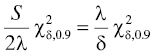
where ![]() is the 90th percentile of the chi-squared distribution on δ degrees of freedom. In most cases, δ will not be an integer, so interpolation between the nearest integers is used. If a UCL other than 90% is desired, change 1.282 to the appropriate confidence coefficient as found in Table 3.4.
is the 90th percentile of the chi-squared distribution on δ degrees of freedom. In most cases, δ will not be an integer, so interpolation between the nearest integers is used. If a UCL other than 90% is desired, change 1.282 to the appropriate confidence coefficient as found in Table 3.4.
Table 3.4 Confidence Coefficients for UCL Computations
| Confidence Level (%) | Confidence Coefficient |
| 90 | 1.282 |
| 95 | 1.645 |
| 99 | 2.326 |
We may also consider the use of two-sided confidence limits for λ. These would be useful when the quality of our knowledge about the λi is good as would be the case if ui and λi are close together. The two-sided confidence 90% confidence interval for λ is then
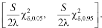
As with the one-sided case, if a confidence level other than 90% is desired, adjust the computation of the si according to Table 3.4. For details of these methods, consult Ref. 6.
Development of a more generally applicable method for confidence intervals for coherent systems with components whose life distributions are other than exponential has been attempted, but no satisfactory method yet exists that is fully applicable and easy to use. Use of the method given here will provide important insight into the quality of knowledge about the reliability prediction for a series system. In particular, this quality of knowledge information is important when using a reliability prediction of this kind to assess the likelihood that the design on which the prediction was made will meet its reliability requirements.
3.4.5 Ensembles Containing Redundant Elements: Parallel Systems
Many practical systems that require high reliability would be impossible to implement if they consisted only of single points of failure. Satellites, aircraft, undersea cable telecommunications systems, and many other systems we have come to accept as an ordinary part of daily life would be less effective without a reliability improvement strategy. Probably the reliability improvement strategy that most people think of first is the provision of spare units that will take over operation when another unit fails. This is called redundancy. Properly done, it can be very effective, but it is also costly and should not necessarily be the first thing the professional reliability engineer thinks of when reliability improvement is needed. This could be an introduction to the interesting and vital field of reliability economics, but that is beyond the scope of this chapter. This section discusses the reliability modeling issues pertaining to redundant systems.
Example: (Continuation of Section 3.4.2.1) An automobile requires four wheels to satisfy one of its most important requirements, namely that it be able to move forward under power provided by its engine. If a wheel fails (e.g., because of a tire puncture and consequent loss of air pressure), the vehicle fails because the requirement that it be able to move under power provided by its engine is violated. Thus each wheel constitutes a single point of failure for the vehicle. But most automobiles carry a spare wheel. When a wheel fails, it is possible to replace it with the spare. Thus, we may consider the spare wheel as a redundant unit that is provided so that the failure of a wheel may be remedied during a mission (driving trip). In the language we will introduce later, the wheel subsystem on the vehicle is a four-out-of-five cold standby redundant system. In the event that a wheel failure has occurred and the failed wheel was replaced by the spare, the vehicle is operating in a brink of failure state until a spare wheel is returned to the vehicle. This example is continued in Exercise 13.
Language tip: When a redundant ensemble operates with no spare units (e.g., all the spares may have been already used to cover failed primary units), we say the ensemble is operating in a brink-of-failure state. The terminology arises from the fact that in this scenario, the next unit failure to occur will cause the ensemble to fail. Some means of detecting when an ensemble is operating in a brink-of-failure state should be provided because if such operation is “silent,” or undetected, failure of the ensemble may occur as a surprise. Provision of a brink-of-failure operation detector is an example of a predictive maintenance procedure; such procedures will be covered in greater detail in Chapter 11.
We examine three kinds of redundancy:
- Hot standby redundancy,
- Cold standby redundancy, and
- k-out-of-n redundancy.
Many more redundancy schemes exist; the reliability engineering literature concerning redundant systems is vast and untamed. In particular, there are many forms of “warm standby” redundancy in which the spare units are considered to be in various intermediate states between operation and complete inactivity. In addition, the reliability of the switching mechanism that implements the redundancy scheme is of great importance, but it is not included in any of the basic models discussed. We will present one example worked out in detail of a two-unit parallel (hot standby) system that includes the reliability of the switching mechanism, but the variety of switching mechanisms is too great to cover all of them completely. We hope that by following the ideas shown in the following example, you will be able to construct suitable models to include switching mechanism reliability when the need arises. Nor will we consider any warm standby models in this book; again, the fundamentals you will learn here will help you use the literature effectively and to model and work with other redundancy schemes when it becomes necessary.
The reliability block diagram for the three redundancy schemes studied here is drawn as a parallel ensemble of units. Figure 3.8 gives an example with four units.
There really is no way to distinguish one scheme from another on the basis of the diagram alone. That is, there is no universally accepted scheme to draw reliability block diagrams for parallel systems that distinguish, on the basis of the drawing alone, the different types of redundancy. The drawing in Figure 3.8 could represent any of the three types of redundancy listed earlier, or even another type (i.e., a warm standby scheme). Labels or color-coding may help when there is ambiguity that needs to be banished, but a universally accepted scheme has not yet been implemented.
3.4.5.1 Hot standby redundancy
The simplest redundancy scheme is hot standby redundancy in which a single unit (the “primary unit”) is supported by one or more “redundant units” (or “backup units”), all of which are powered on and aging along with the primary unit. When the primary unit fails, some switching mechanism operates to bring the failed unit off line and one of the redundant units on line to take over the operation that was being performed by the primary unit before it failed (assuming the switching operation does not fail). Thus, the ensemble fails only when all units, the primary unit and all the redundant units, fail. In the case of hot standby, or active, redundancy, we have for the lifetime L of the ensemble in terms of the lifetimes L1, . . ., Ln of its constituent units, again assuming the switching mechanisms does not fail,
From here, it is a routine matter to obtain the distribution of L:
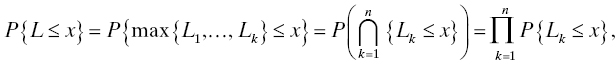
where the last equality is valid if the individual lifetimes are stochastically independent. We may also write
In terms of the survivor functions, we have
Note the duality between the series system discussed in Section 3.4.4 and the hot-standby parallel system discussed here: in the series system, the expression for the life distribution looks like the expression for the survivor function of a hot-standby parallel system, and vice versa.
Example: A Two-Unit Hot Standby Redundancy Arrangement with an Unreliable Switch
Consider the hot standby arrangement depicted in Figure 3.9.

Figure 3.9 Two-unit hot standby ensemble with switch.
Denote by L1 and L2 the lifetimes of the first (topmost in the figure) and second units, respectively, let the corresponding survivor functions be denoted by S1 and S2, and denote by L the lifetime of the entire ensemble. Let W(t) denote the indicator of the event that the switch operates correctly when it is called upon to do so at time t, let p(t) = P{W(t) = 1}, and Zt denote the lifetime of the switch given that it operates correctly at time t (if the switch fails to operate correctly when called for, then L = L1 and the value of Zt is irrelevant). Furthermore, we assume there is no “rejuvenation” of the switch if it fails when called for: once this failure occurs, the ensemble is failed. Let Gt denote the life distribution of Zt. If there were no switch involved (usually not feasible in an engineering sense), then L would be equal to max{L1, L2}, and the life distribution at time t of the ensemble would be F1(t)F2(t). If the switch operation were perfectly reliable (i.e., p(t) ≡ 1 for all t), then L would be equal to the maximum of L1, L2, and min{L1, L2} + min{ZT, max{L1, L2}} because the switch will be called for at time T = min{L1, L2}. In this case, the survivor function of L would be
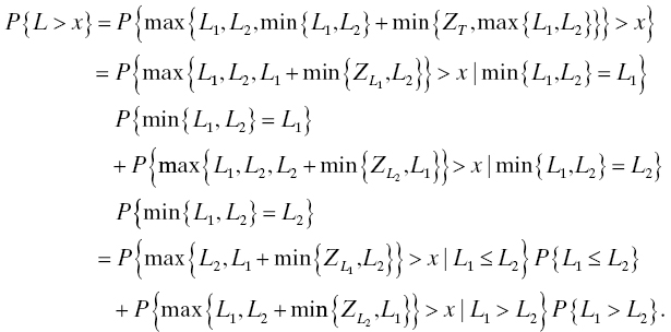
Now
assuming that L1 and L2 are independent, and the distribution of ![]() is equal to
for i = 1, 2, assuming that L1 and L2 are conditionally independent of Zt for all t. These may now be substituted into the expression above for P{L > x} to complete the development (see Exercise 16). In case the switching action may be unreliable (i.e., p(t) < 1 for at least one t), then the survivor function of L is given by
is equal to
for i = 1, 2, assuming that L1 and L2 are conditionally independent of Zt for all t. These may now be substituted into the expression above for P{L > x} to complete the development (see Exercise 16). In case the switching action may be unreliable (i.e., p(t) < 1 for at least one t), then the survivor function of L is given by
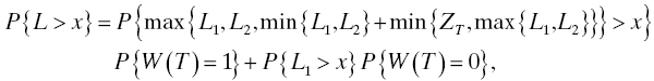
again assuming the necessary independence (in this case, that of W(T) from everything else in sight).
Requirements tip: It is clear from this example that reliability models that include imperfect switching for redundant systems may be considerably more complicated than those that ignore the effect of potentially unreliable switching. Systems engineers need to be aware that switching mechanism unreliability can be a significant contributor to overall system unreliability in cases where redundancy is being used to increase system reliability overall. Be sure that reliability engineers on the project provide realistic reliability projections in these cases because the high cost of redundancy can be rendered for naught by a relatively low-cost switching mechanism that may be unreliable.
3.4.5.2 Cold standby redundancy
Cold standby, or passive, redundancy differs from hot standby redundancy in that the redundant units are not active while the primary unit is in service. This model postulates that the standby units do not age while they are not operating, that is, the “lifetime clock” does not start for these units until they are put into service. When the primary unit fails, the switching operation activates the first redundant unit and takes the failed unit off line, and puts the now-active redundant unit on line so that the ensemble continues to perform its function. In this case, the lifetime of the ensemble is the sum of the lifetimes of all its constituent units (again assuming that all the switching operations are perfect). That is,
To find the distribution of L when the lifetimes L1, . . ., Ln are independent, we introduce the notion of convolution of distribution functions. Suppose X and Y are independent lifetimes having distributions F and G, respectively. Then the distribution of X + Y is given by
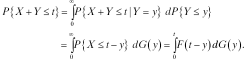
The last integral is called the convolution of F and G and is denoted F*G(t). Thus, if F1, . . ., Fn represent the life distributions of L1, . . ., Ln, respectively, then the life distribution of the cold standby ensemble is given by F1* ⋅ ⋅ ⋅ *Fn. The family of gamma distributions is closed under convolution. As was noted in Section 3.3.4.7, the sum of two independent random variables having gamma distributions with parameters (α1, ν) and (α2, ν) again has a gamma distribution with parameters (α1 + α2, ν). So a cold standby redundant system whose first unit’s lifetime has a gamma distribution with parameters (α1, ν) and whose second unit’s life distribution has a gamma distribution with parameters (α2, ν) has a life distribution with parameters (α1 + α2, ν). In most other cases, it is not possible to evaluate convolution integrals in closed form. Various numerical methods have been developed to enable computation of system reliability when cold standby redundancy is present. Among the simplest are the Newton–Cotes-like rules found in Ref. 54.
The number and variety of reliability models for imperfect switching incorporated into cold standby redundancy schemes is at least as great as the large number of such schemes. We will consider only a simple example to illustrate some possibilities. Suppose that in an n-unit cold standby redundancy scheme there is a switching mechanism whose duty is to switch in the next unit when the unit currently in service fails, and suppose that the indicator event that this switch performs its duty correctly when called upon at time t is W(t), independent of everything else, P{W(t) = 1} = p(t), and if W(t0) = 0, then W(t) = 0 for all t ≥ t0. Further suppose that the lifetime of the switch is infinite (i.e., the switch does not fail once the switching operation has completed successfully—the only possible failures of the switch are at the moments of switching). Then the life distribution of the ensemble is
See Exercise 17 to complete this example.
3.4.5.3 k-out-of-n redundancy
The final type of redundancy we study in this chapter is the k-out-of-n scheme. In this scheme, there are n units. The ensemble operates if and only if k of these n units are in an operating condition. One may think of this as a system that requires k units to operate properly and that has in addition n − k spare units on site. This scheme may be implemented as hot standby or cold standby (and other types of warm standby which will not be covered here). In a hot standby arrangement, the lifetime of the ensemble is the kth shortest of the n unit lifetimes. This is an example of an order statistic. The life distribution of the hot standby k-out-of-n ensemble is the cumulative distribution of this order statistic which may be found in Ref. 14.
In a cold standby k-out-of-n scheme, the lifetime is determined by counting the total number of unit failures that occur by a given time. The first time this reaches n − k + 1 is the time of ensemble failure. Let N(t) represent the number of unit failures in the time interval [0, t], and let L represent the system lifetime. Then the “counting argument” is that the time to system failure occurs after time t if and only if there have been no more than n − k unit failures up to and including time t,
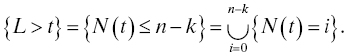
Our task will be to obtain the distribution of L as

We will now assume that all primary units have the same reliability characteristics, all standby units have the same reliability characteristics (although these may be different from the primary units), and all units are mutually stochastically independent. We begin by defining the concept of “position.” Consider the primary units that are started operating at time zero. The location or “slot” that each of these occupies is called a “position.” At the time a primary unit fails, a spare unit is immediately placed in service in that position (the pool of spares initially contains n − k units; if this is the (n − k + 1)st failure in a primary slot, then the ensemble fails at this time and there are no spare units remaining in the pool). Thus, we record the failures in each “position” separately, or, in other words, each “position” is thought of as having a failure process of its own. To illustrate the idea, we will first work through the derivation in the simple case n = 2, k = 1. In this case, denoting by N1(t) the number of failures in position 1 that occur during [0, t], we have P{L > t} = P{N1(t) ≤ 1}, because the system fails when the second failure in position 1 occurs. Define T = inf {t : N(t) = 1} and T + S = inf{t : N(t) = 2}. Thus, P{N(t) ≤ 1} = P{T + S > t} = 1 − F*G(t). Obviously, in this case we have L = T + S, so there was really no need to go through the counting argument, but it is valuable to see how it works in this simple case first. In the general case, let Ni(t) denote the number replacements in position i by spare units, i = 1, . . ., k. Then we have ![]() because the spare units only operate (and fail) in the primary (first k) positions. This gives us the opening we need to get the distribution of N(t). Define W0(t) = 0 and
because the spare units only operate (and fail) in the primary (first k) positions. This gives us the opening we need to get the distribution of N(t). Define W0(t) = 0 and ![]() . Then W1(t) = N1(t) and Wk(t) = N(t). Using the relation Wi(t) = Wi−1(t) + Ni(t), i = 1, . . ., k, and the mutual independence of N1(t), . . ., Nk(t), we can get the distribution of each Wi(t) by successive discrete convolutions:
. Then W1(t) = N1(t) and Wk(t) = N(t). Using the relation Wi(t) = Wi−1(t) + Ni(t), i = 1, . . ., k, and the mutual independence of N1(t), . . ., Nk(t), we can get the distribution of each Wi(t) by successive discrete convolutions:

To model the failure counting processes Ni(t), i = 1, . . ., k, in the k primary positions, we assume that the primary units are identical, and all have life distribution F, say, and the spare units are identical, and all have life distribution G, say. Then we have P{Ni(t) = 0} = 1 − F(t), i = l, . . ., k, and
Here, Gj−1 represents the convolution of G with itself j − 1 times, and G0 is the unit step function at the origin. Working backward to the equation for P{L ≤ t} completes the derivation.
3.4.6 Structure Functions
In Section 3.4.3, we saw how to express pictorially the “reliability logic” of a system by using the reliability block diagram. We may also summarize the reliability logic of a system using a concept called the structure function.19 The reliability logic of a system is a catalog of how system failure results from component failures. For instance, in the ensemble of single points of failure (the series system), the system fails whenever a component fails. The structure function is a mathematical representation of this logic. It is a Boolean function (its arguments and values come from {0, 1} only); in this formalism, 1 is taken to mean the component or system is in an operating state and 0 is taken to mean the system is in a failed state. If Ci is the indicator that component i is working (i.e., Ci = 1 if component i is working and is 0 otherwise), then the system structure function is φR(C1, . . ., Cn) where C1, . . ., Cn is the list of (indicator functions of) the components of the system. φR is the indicator that the system is working; the functional form in terms of the C1, . . ., Cn tells whether the system works when its constituent components are working or failed. Sometimes, the vector (C1, . . ., Cn) is called the vector of component states or the state vector.
For example, the structure function of an ensemble of single points of failure (a series system) is φR(C1, . . ., Cn) = C1 ⋅ ⋅ ⋅ Cn because φR(C1, . . ., Cn) is 1 if and only if all the Ci are 1. As soon as one of the Ci is zero, the structure function is zero. This is the logic of the series system (the system fails if and only if at least one of its components fails) expressed in mathematical terms. The structure function of a parallel (hot standby) system is given by φR(C1, . . ., Cn) = 1 − [(1 − C1) ⋅ ⋅ ⋅ (1 − Cn)]. The structure functions of ensembles comprising components in nested series and parallel configurations are readily expressible. See Exercise 18.
If we now allow the structure function and its arguments to take values in [0, 1], we obtain a simple expression for the probability that the system operates as a function of the probabilities of each component operating [9] . We can use this idea to write an expression for the survivor function of the system in terms of the survivor functions of its constituent components. Let S1, . . ., Sn denote the survivor functions of components C1, . . ., Cn, respectively, and let S denote the system’s survivor function. Then for each time t,
A disadvantage of the structure function approach is that it is not easily possible to incorporate warm standby and cold standby redundancy into the structure function scheme. On the other hand, for systems not having these methods implemented, the structure function approach provides a compact and mathematically convenient approach to working with complex structures. Additional properties of structure functions are explored in detail in Refs. 5, 19.
3.4.7 Path Set and Cut Set Methods
The graph metaphor for reliability block diagrams was introduced in Section 3.4.3. Methods for determining the reliability of ensembles of single points of failure and ensembles with redundancy were reviewed in Sections 3.4.4 and 3.4.5. These methods rely heavily on the simple nature of the reliability block diagram graph when it can be represented in “series” or “parallel” form. Here we discuss some methods for determining the reliability of the diagram as a function of the reliabilities of its constituent components when the reliability block diagram graph is more complicated (not in “series” or “parallel” form). Most of this material originally appeared in Ref. 59 and is reprinted here with permission. This section reviews the concepts of connectedness, paths, cuts, path sets, and cut sets in the context of analyzing a system reliability block diagram described as a labeled random graph. The methods discussed also lend themselves to the development of bounds for system reliability. More general interpretations of this material can also be used to define and determine reliability for capacitated networks [50].
A graph is an ordered pair of sets (![]() ,
, ![]() ) :=
) := ![]() with
with ![]() ⊂
⊂ ![]() ×
× ![]() .
. ![]() is called the set of nodes of the graph and
is called the set of nodes of the graph and ![]() is called the set of links of the graph. Typically, a graph is pictured as a drawing in which the nodes are represented as points in the plane and the links are represented as lines drawn to join two points. In other terminology in common use, the nodes may be called vertices and the links may be called arcs or edges. A labeled graph is a graph in which the nodes and/or links have names. That is, there is a one-to-one correspondence between the nodes of the graph and a set of |
is called the set of links of the graph. Typically, a graph is pictured as a drawing in which the nodes are represented as points in the plane and the links are represented as lines drawn to join two points. In other terminology in common use, the nodes may be called vertices and the links may be called arcs or edges. A labeled graph is a graph in which the nodes and/or links have names. That is, there is a one-to-one correspondence between the nodes of the graph and a set of |![]() | objects (the node labels) and/or between the links of the graph and a set of |
| objects (the node labels) and/or between the links of the graph and a set of |![]() | objects (the link labels). A directed graph is a graph in which each link is assigned an orientation or direction. In a directed graph, the links (i, j) and (j, i) are different, whereas in an ordinary (undirected) graph, they are identical. The concept of “a link from i to j” makes sense in a directed graph; in an undirected graph, it would be proper to say, rather, “a link between i and j.”
| objects (the link labels). A directed graph is a graph in which each link is assigned an orientation or direction. In a directed graph, the links (i, j) and (j, i) are different, whereas in an ordinary (undirected) graph, they are identical. The concept of “a link from i to j” makes sense in a directed graph; in an undirected graph, it would be proper to say, rather, “a link between i and j.”
Two nodes i and j are adjacent if (i, j) ∈ ![]() . A path in a graph is a sequence of adjacent nodes and the links joining them, beginning and ending with a node. Two nodes i and j are said to be connected if there is a path having i as its initial node and j as its terminal node. That is, the path takes the form {i, (i, ν1), ν1, (ν1, ν2), . . ., νk, (νk, j), j} for some ν1, . . ., νk ∈
. A path in a graph is a sequence of adjacent nodes and the links joining them, beginning and ending with a node. Two nodes i and j are said to be connected if there is a path having i as its initial node and j as its terminal node. That is, the path takes the form {i, (i, ν1), ν1, (ν1, ν2), . . ., νk, (νk, j), j} for some ν1, . . ., νk ∈ ![]() and (i, ν1), (ν1, ν2), . . ., (νk, j) ∈
and (i, ν1), (ν1, ν2), . . ., (νk, j) ∈ ![]() . There is no loss in abbreviating this to {i, ν1, ν2, . . ., νk, j}. When it is necessary or desirable to explicitly indicate the nodes being connected, the path will be called an (i, j)-path. Clearly, adjacent nodes are connected, but connected nodes need not be adjacent. If the graph is directed, the links in the path must be considered with the proper orientation. A path connecting two given nodes is called minimal if it contains no proper subset that is also a path connecting the two nodes.
. There is no loss in abbreviating this to {i, ν1, ν2, . . ., νk, j}. When it is necessary or desirable to explicitly indicate the nodes being connected, the path will be called an (i, j)-path. Clearly, adjacent nodes are connected, but connected nodes need not be adjacent. If the graph is directed, the links in the path must be considered with the proper orientation. A path connecting two given nodes is called minimal if it contains no proper subset that is also a path connecting the two nodes.
A cut for two given nodes is a set of nodes and/or links whose removal from the graph disconnects the two nodes. To explicitly indicate the nodes being disconnected, the cut may be called an (i, j)-cut. A cut for two given nodes is called minimal if it contains no proper subset that is also a cut disconnecting those nodes.
The Washington, DC, Metro subway system [32] may be modeled as a graph with the stations as the nodes. In this graph, the Pentagon and College Park–University of Maryland stations are connected but not adjacent. DuPont Circle and Farragut North are both connected and adjacent. The (Takoma, Union Station) path is a cut for the Silver Spring and Judiciary Square nodes. It is not a minimal cut because its subset (Brookland–CUA, Rhode Island Avenue) is also a cut for the Silver Spring and Judiciary Square nodes. See Exercise 26.
A random graph is a labeled graph in which the labels are stochastic indicator variables. When the variable is zero, it indicates that that node or link is not present in the graph. When it is one, it indicates that that node or link is present in the graph. Each choice of values for these indicator variables, by whatever random mechanism is at play, produces a different graph (the choice is not completely unrestricted; if the indicator of a node is zero, the indicators of all the links emanating from that node must be zero also). In the reliability modeling application, the indicator variable for a link or node describes the functioning or nonfunctioning of the link or node. The usual convention is that the indicator variable is 1 when the link or node functions and 0 when it does not function.
The system reliability block diagram is a labeled random graph whose nodes represent the components or subsystems whose reliability description is known or provided. The links are merely connectors and may be disregarded for these purposes.20 The system reliability block diagram expresses the reliability logic of a system in the sense that it shows how the system fails when constituent components and subsystems fail. It is a pictorial representation of the system structure function. Two special nodes are called out: a source, or origin, node, and a terminal, or destination, node. The system functions if and only if in the random graph there is a path connecting the source node and the terminal node.
In many cases, the system reliability block diagram is a series-parallel structure. In such cases, the probability that the system functions is easily concluded from nesting of the standard formulas for the reliability of series systems and parallel systems (see Sections 3.4.4 and 3.4.5). Other structures, such as the k-out-of-n hot standby and k-out-of-n cold standby structures, are also amenable to similar probabilistic analysis as seen earlier. Some other structures, such as the bridge structure shown in Figure 3.10, lend themselves less readily to this type of analysis. In such cases, it may be convenient to use the path set or the cut set methods described here.
Figure 3.10 Bridge network.
In the bridge network, the source is node 1 and the terminal is node 4. The (1, 4) paths are {1, 2, 4}, {1, 3, 4}, {1, 2, 3, 4}, and {1, 3, 2, 4} and the minimal paths are {1, 2, 4} and {1, 3, 4}. The (1, 4) cuts are {1}, {4}, {1, 2}, {1, 3}, {2, 4}, {3, 4}, {2, 3}, {1, 2, 3}, {2, 3, 4}, and {1, 2, 3, 4}. The minimal cuts are {1}, {4}, and {2, 3}.
Given two nodes in a graph, the path set (sometimes called tie set) for those two nodes is the set of all paths connecting those two nodes. The cut set for two nodes is the set of all cuts for those two nodes. The minimal path set for a pair of nodes is the set of all minimal paths for that pair of nodes. The minimal cut set for a pair of nodes is the set of all minimal cuts for that pair of nodes. The key concepts for reliability modeling are
- The system functions if and only if there is at least one minimal path whose components are all in a functioning condition and
- The system does not function if and only if there is as least one minimal cut whose components are all in a failed (nonfunctioning) condition.
The random graph model provides a framework for computing probabilities of system functioning and failure (nonfunctioning) based on these concepts.
Example: Consider the reliability block diagram shown in Figure 3.11. The nodes representing subsystems that can fail individually in this system have been labeled by the letters A, B, C, and D. Note that, like the bridge structure of Figure 3.10, this is not a series-parallel graph, so the methods of Section 3.4.3 do not apply. In this model, the system functions if the node s at the left-hand edge of the diagram and the node t at the right-hand edge of the diagram are connected. This representation indicates that the system functions if any one of the sets {A, B}, {A, D}, {C, B}, {C, D}, {A, B, C}, {A, C, D}, {B, C, D}, {A, B, D}, or {A, B, C, D} consists entirely of functioning units. Each of these is an (s, t)-path. The union of these nine paths constitutes the path set for the node pair (s, t). Note that not all these paths are minimal; for example, C can be removed from {A, B, C} and the result {A, B} is still an (s, t)-path. The minimal paths are {A, B}, {A, D}, {C, B}, and {C, D}, so {{A, B}, {A, D}, {C, B}, {C, D}} is the minimal path set. Similarly, the system fails to function if any of the sets {A, C}, {B, D}, {A, C, B}, {A, B, D}, {A, C, D}, or {A, B, C, D} consists entirely of nonfunctioning, or failed, units. Any one of these is an (s, t)-cut. The minimal (s, t)-cuts are {A, C} and {B, D}. The minimal cut set for (s, t) is {{A, C}, {B, D}}.
Figure 3.11 Example of a system reliability block diagram.
Because the path set contains all paths connecting s to t, for the system to function, it suffices that at least one path be made up entirely of functioning units. Therefore, the probability that the system functions is given by the probability of the path set in the labeled random graph representing the system reliability block diagram. However, only minimal paths need be considered because if a path is not a minimal path, then it has a proper subset that is still a path and is a member of the minimal path set. In other words, the union of all (s, t)-paths is equal to the union of all (s, t)-minimal-paths. Consequently, the probability that the system functions is given by the probability of the system’s minimal path set. In general, the minimal paths will not be disjoint, so some version of the inclusion–exclusion formula [12] will have to be used to compute this probability.
Example (cont’d): Consider again the system shown in Figure 3.11. Letting pA = P{A = 1} (where we have abused notation slightly by identifying the indicator random variable’s letter with the unit’s label) and similarly for B, C, and D, the probability that the system functions is given by
This equation illustrates the strength and weaknesses of the path set method. Its strength is that it is completely straightforward and mechanical to write the expression for the probability that the system functions once the minimal path sets are known. Its weaknesses are that (1) enumerating the paths connecting s and t is tedious for all but the simplest of graphs, and (2) the expression that results is the probability of a large union of events that are not, in general, disjoint. However, these weaknesses pertain mainly to manual execution; the algorithmic nature of the procedure means that software for path set reliability analysis is within reach, and indeed has been available for some time [23, 40, 63].
For the general representation of system reliability using the minimal path set, let x = (x1, . . ., xc) denote the vector of indicators of the functioning of the c components of the system. Enumerate the minimal paths of the system; suppose there are m of them called π1, . . ., πm. Assuming independence of the units, the probability that the series system represented by the minimal path πk is working is given by
for k = 1, . . ., m. The system functions if and only if at least one of the minimal paths consists entirely of functioning units, so it follows that the system reliability may be written as

This equation shows how the system structure function may be represented in terms of the structure functions of the system’s minimal paths.
Because the cut set contains all (s, t)-cuts, for the system to fail it is necessary and sufficient that at least one cut be made up entirely of nonfunctioning units. However, only minimal cuts need be considered because if a cut is not a minimal cut, then it has a proper subset that is still a cut and is a member of the minimal cut set. In other words, the union of all (s, t)-cuts is equal to the union of all (s, t)-minimal-cuts. Therefore, the probability that the system fails to function is given by the probability of the minimal cut set in the labeled random graph representing the system reliability block diagram. Consequently, the probability that the system fails is given by the probability of the system’s minimal cut set.
Example (cont’d): Consider again the system shown in Figure 3.11. The probability that the system fails to function is given by
While this expression simplifies quickly because the two events in the union are disjoint, in general the expression that results from minimal cut set analysis will contain events that are not disjoint so that computation can become cumbersome. An algorithm for system reliability evaluation using cut sets may be found in Ref. 19.
For the general representation of system reliability via minimal cut set analysis, enumerate the minimal cuts χ1, . . ., χn of the system. The probability that the series system represented by the minimal path χk consists entirely of nonfunctioning units is given by
for k = 1, . . ., n. The system fails if and only if at least one of the minimal cuts consists entirely of nonfunctioning units, so it follows that the probability that the system fails may be written as
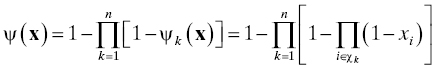
Additional information on the use of path sets and cuts sets for system reliability modeling and computation may be found in Refs. 3, 49.
The minimal path set and minimal cut set representations for the system reliability lend themselves readily to the development for bounds on the system reliability. The first such bounds were developed by Esary and Proschan [19] . Letting C (resp., W) denote the minimal cut (resp., minimal path) set for the system, that is, for the nodes (s, t), Esary and Proschan’s bounds for the system reliability R are

The lower bound gives good approximations for highly reliable systems, while the upper bound works better for systems whose components have low reliability. Numerous improvements have been developed (see Refs. 22, 39 for further developments).
3.4.8 Reliability Importance
When designing for reliability, it is useful to expend resources on the parts of the system whose improvement causes the greatest improvement in system reliability. The concept of reliability importance formalizes this notion. The earliest definition of reliability importance was given by Birnbaum [8] . The reliability importance of component i in a system whose structure function is φR(x1, . . ., xn) is the partial derivative of φR with respect to xi, evaluated at x1, . . ., xn. For example, for a series system containing n components (single points of failure) having reliabilities x1, . . ., xn, the reliability importance of component i is

from which it can be seen that the least reliable component is the most important, that is, the one whose improvement would result in the greatest improvement of the system reliability.
Many other definitions of reliability importance, adapted to other applications, have been proposed [11] . Deeper discussion of reliability importance is beyond the scope of this chapter. Readers interested in pursuing this topic further would be well served by beginning with Ref. 11.
3.4.9 Non-Service-Affecting Parts
It may happen that some components of a system are irrelevant to system failure, that is, failure of one of these components has no effect on the operation of the system. Failure of the component is not only invisible when it happens but also it does not increase the load on other components. Obviously, this is an unusual situation, limited to such items as decorative trim, serial number labels, and so on. It is often obvious that components of this kind are not part of the system functional description and do not belong as part of the system reliability block diagram or the system structure function. In the mathematical theory of reliability [4], systems that contain irrelevant parts are called noncoherent.21 Such components are also called non-service-affecting. The reliability importance (Section 3.4.8) of such parts is zero.
Unless there is a requirement for continued operation of decorative trim! This is not entirely facetious. For example, many electronic systems contain power supply bypass capacitors. Should one of these fail open (i.e., in such a way that the failed capacitor looks like an open circuit), usually no noticeable difference in operation can be discerned, and a single bypass capacitor may be considered a non-service-affecting part. The failure may cause increased noise on the power bus, and if enough bypass capacitors fail open, then the level of noise may increase to a point where a system bit error rate requirement may be violated, for example. Careful analysis may be required to determine the number of such failures tolerable before noise becomes an issue for other requirements. When this number is determined, the bypass capacitors may be incorporated into a system reliability block diagram as a k-out-of-n ensemble in series with the rest of the diagram, where n is the total number of such bypass capacitors in the system and n − k is the number of (open) failures that need to occur before they are noticeable. Of course, there is another failure mode for capacitors, and that is to fail short (i.e., in such a way that the failed capacitor looks like a short circuit). A short failure should lead to a blown fuse, or, if the power supply is not properly fused, a short failure can lead to failure of other power supply components or even cause the power supply to catch fire.
3.5 RELIABILITY MODELING BEST PRACTICES FOR SYSTEMS ENGINEERS
We defer this discussion until the end of Chapter 4 when we have covered reliability modeling for maintained systems also.
3.6 CHAPTER SUMMARY
This chapter has provided background material on reliability modeling systems engineers need in order to be good customers and suppliers in the development process. It is possible to use this chapter as a framework for advanced study of reliability modeling, but its primary intent is to equip systems engineers to be effective in dealing with the reliability engineering aspects of product and service development.
The chapter covers reliability effectiveness criteria and reliability figures of merit used for nonrepairable systems. Those in most common use are mission survivability and lifetime for nonrepairable systems. We caution extra care around “failure rate.” The phrase is used for several different concepts, some of which require special conditions, so you need to be aware of which meaning is intended in any particular case.
3.7 EXERCISES
- Suppose the strength of a population of devices is characterized by a random variable S having density fV. Suppose the environment presents this population of devices with stresses ∑i occurring at times Ti, i = 1, 2, . . ., where {T1, T2, . . .} is a homogeneous Poisson process with rate τ and ∑i are independent and identically distributed random variables having density gV. Determine the distribution of time to failure for a device chosen at random from this population subjected to these stresses.
- Let F(x) = 1 − exp((−x/α)β) for x ≥ 0 and F(x) = 0 for x < 0, where α and β are positive constants. Show that F has the four properties of a life distribution listed in Section 3.3.2.3.
- Show that the gamma distribution has a decreasing hazard rate when 0 < ν < 1.
- Discuss the distribution F(x) = 1 − exp(−αxβ) where x ≥ 0 and α and β are positive constants. Compare with Exercise 2.
- Consider an ensemble of three single-point-of-failure components. The lifetime of the first component has an exponential distribution with parameter 0.001 failures per hour. The lifetime of the second component has a Weibull distribution with parameters 0.001 and 1.7, and the lifetime of the third component has a lognormal distribution with parameters 0.005 and 2.3. If the components are considered stochastically independent, what is the probability that the ensemble survives at least 40,000 hours? What information would be required to solve this problem if the components are not considered stochastically independent?
- Derive the force of mortality for the uniform distribution on [a, b] and show that it becomes infinite as x → a + and x → b −. For a life distribution that has finite support [a, b] with 0 ≤ a < b < ∞ and that has a hazard rate, determine sufficient conditions for the hazard rate to become infinite as x → b −.
- Write expressions for the life distribution and density corresponding to the Holcomb and North hazard rate model described in Section 3.3.4.4.
- Show that, under the strong or weak accelerated life models, if the life distribution at nominal conditions has a certain parametric form, then the life distribution at any altered conditions continues to have the same parametric form.
- Suppose a power supply choke inductor has a life distribution given by F(t) = 1 − exp(−(t/18,000)0.9), where t is measured in hours, when the ambient temperature is 15°C. Use the differential accelerated life model to determine the life distribution of the inductor when the operational temperature environment is 20°C with a diurnal variation of ±6°C. (Hint: represent the temperature environment as T(t) = 20 + 6sin(πt/12)).
- Suppose the system shown in Figure 3.9 is a cold standby system. Find the life distribution of the system in case
- the switch is perfect and
- the switch many fail.
- Show that the force of mortality for the life distribution of a series system of an arbitrary (finite) number of components is the sum of the individual forces of mortality for the life distribution of each component. Is independence necessary? Is identical distribution necessary?
- Find the cut sets and minimal cut sets for the reliability block diagram in Figure 3.10.
- Develop further the example given in Section 3.4.1. Is it appropriate to consider the spare unit as a cold standby unit? What role does the replacement time (i.e., the time it takes to replace the failed wheel with the spare) play in the scenario? What are the consequences of the spare’s being improperly inflated?
- Consider a two-unit hot standby redundant system. Write an expression for the lifetime of this system in terms of its constituent component lifetimes when the switching mechanism may be imperfect (i.e., may fail when called for).
- Find the life distribution of a two-out-of-three hot standby ensemble. Do the same for a two-out-of-three cold standby ensemble. Compare your results with the two-out-of-four and the three-out-of-four cases.
- Complete the derivation of the survivor function shown in the example of a two-unit hot standby redundancy arrangement with an unreliable switch given in Section 3.4.5.1.
- Complete the development of the life distribution of the cold standby ensemble with imperfect switching example given in Section 3.4.5.2.
- Write the structure function for an ensemble consisting of a component in series with a parallel system of three components.
- Regenerators for fiber-optic telecommunications systems are frequently located in remote, difficult-to-access areas. Consequently, a spare regenerator that is switched in automatically is provided for each active regenerator so that should the active regenerator fail, it is not necessary to incur the expense of sending a technician out to repair or replace the failed regenerator. The switching mechanism comprises a detection circuit (to determine that the active regenerator has failed), a switching mechanism to substitute the spare regenerator for the failed regenerator, and a communication mechanism that alerts (remote) staff to the success or failure of the switch when the active regenerator fails.
- Should this be a hot standby or cold standby scheme? Discuss the advantages and disadvantages of each. How would you make this decision?
- Make a reliability model for the switching mechanism.
- Make a reliability model for the ensemble of the two regenerators and switch that is consistent with your solution to part (a).
- Make a sensitivity study of the reliability of the ensemble as a function of your assumptions about the reliabilities of the components of the switching mechanism.
- Write requirements for the reliability of the major components of the ensemble (the regenerators and switch components). Is there a reasonable way to do this if you do not yet have an overall system reliability requirement (i.e., a reliability requirement for the entire fiber-optic route of which this ensemble is a part)? How would your solution to part (d) contribute to the necessary understanding of the reliability economics of this ensemble and to the negotiation of reliability requirements with the systems engineer for the entire route?
- Suppose a population of devices has a life distribution that is Weibull with parameters α = 10,000 and β = 2. Find the expected number of device failures in the time intervals [500k, 5000(k+1)] for k = 1, 2, . . ., 10. What is the probability that a device fails in each interval, given that it is alive at the beginning of the interval? What is the expected number of device failures in each interval among the devices that are still alive at the beginning of the respective intervals?
- In the Example of Section 3.3.4.8, suppose the loss of material follows a normal distribution with mean 2.5 and standard deviation 1.5 instead of the uniform distribution illustrated in the example. Repeat the steps in the example to show that the resulting life distribution of the population of ball bearings has an increasing hazard rate. Does the normal distribution assumption make sense here? Discuss.
- Determine the relationships between the densities at the nominal and the operating conditions, and between the distributions at the nominal and the operating conditions, for the Cox proportional hazards model (Section 3.3.5.2).
- Develop the model given in Section 3.3.6 to a product requiring two manufacturing processes. How would your solution generalize to more than two processes?
- Use the Maclaurin series for log(1 − y) to show that −y 2/2 ≤ y + log(1 − y) ≤ 0 for 0 ≤ y ≤ 1.
- Consider a lot of 200 circuit packs, each containing 10,000 solder attachments, manufactured by a wave soldering process whose lower and upper specification limits are aL and aU, respectively. Suppose that F(x, a) = 0 for aL ≤ a ≤ aU and F(x, a) = 1 − exp(−λx), independent of a, whenever a ∉ [aL, aU]. Suppose further that the wave-soldering process just meets the six-sigma criteria (i.e., m = 4.5 or 7.5 in Section 3.3.6). Provide a lower bound and an upper bound on the survivor function for the solder attachments in this population of 200 circuit packs. How might you create a more realistic mathematical model of this process? Would it make a great deal of difference to the results?
- Identify the cut sets and minimal cut sets for the Metro Central and Fort Totten nodes in the Washington, DC, Metro subway system.
REFERENCES
- 1. Abramowitz M, Stegun IA. A Handbook of Mathematical Functions with Formulas, Graphs, and Mathematical Tables. Washington: National Bureau of Standards; 1964.
- 2. Ascher H, Feingold H. Repairable Systems Reliability: Modeling, Inference, Misconceptions, and their Causes. New York: Marcel Dekker; 1984.
- 3. Barlow RE, Proschan F. Statistical Theory of Reliability and Life Testing: Probability Models. New York: Holt, Rinehart, and Winston; 1975.
- 4. Barlow RE, Proschan F. Mathematical Theory of Reliability. Philadelphia: SIAM Press; 1996.
- 5. Baxter LA. Availability measures for a two-state system. J Appl Prob 1981;18:227–235.
- 6. Baxter LA. Towards a theory of confidence intervals for system reliability. Stat Probab Lett 1993;16 (1):29–38.
- 7. Baxter LA, Tortorella M. Dealing with real field reliability data: circumventing incompleteness by modeling and iteration. Proceedings of the 1994 Reliability and Maintainability Symposium; 1994. p 255–262.
- 8. Birnbaum ZW. On the importance of different components in a multicomponent system. Technical report TR-54, Washington University (Seattle) Laboratory of Statistical Research; 1968.
- 9. Birnbaum ZW, Esary JD, Saunders SC. Multi-component systems and structures and their reliabilities. Technometrics 1961;3:55–77.
- 10. Bogdanoff JL, Kozin F. Probabilistic Models of Cumulative Damage. New York: John Wiley & Sons; 1985.
- 11. Boland PJ, El-Neweihi E. Measures of component importance in reliability theory. Comput Oper Res 1995;22 (4):455–463.
- 12. Chung K-L. A First Course in Probability. New York: Academic Press; 2001.
- 13. Cox DR. Analysis of Survival Data. London: Chapman and Hall; 1984.
- 14. David HA. Order Statistics. New York: John Wiley & Sons, Inc; 1970.
- 15. Drenick RF. The failure law of complex equipment. J Soc Indust Appl Math 1960;8 (4):680–690.
- 16. Elsayed EA. Reliability Engineering. 2nd ed. Hoboken: John Wiley & Sons, Inc; 2012.
- 17. Engel E. A Road to Randomness in Physical Systems. Volume 71, New York: Springer-Verlag; 1992.
- 18. Engelmaier W. 2008. Solder joints in electronics: design for reliability. Available at https://www.analysistech.com%2Fdownloads%2FSolderJointDesignForReliability.PDF. Accessed November 12, 2014.
- 19. Esary JD, Proschan F. Coherent structures of non-identical components. Technometrics 1963;5:191–209.
- 20. Escobar LA, Meeker WQ. A review of accelerated test models. Stat Sci 2006;21 (4):552–577.
- 21. Feller W. An Introduction to Probability Theory and its Applications. 2nd ed. Volume II, New York: John Wiley & Sons, Inc; 1971.
- 22. Fu JC, Koutras MV. Reliability bounds for coherent structures with independent components. Stat Probab Lett 1995;22:137–148.
- 23. Gebre BA, Ramirez-Marquez J. Element substitution algorithm for general two-terminal network reliability analyses. IIE Trans 2007;39:265–275.
- 24. Gertsbakh I, Kordonskiy K. Models of Failure. Berlin: Springer-Verlag; 1969.
- 25. Grigelionis B. On the convergence of sums of random step processes to a Poisson process. Theory Probab Appl 1963;8 (2):177–182.
- 26. Grubbs FE. Approximate fiducial bounds for the failure rate of a series system. Technometrics 1971;13:865–871.
- 27. Gumbel EJ. Statistics of Extremes. Mineola: Dover Books; 2004.
- 28. Gupta R, Goel R. The truncated normal lifetime model. Microelectron Reliab 1994;34 (5):935–937.
- 29. Harry MJ. The Nature of Six-Sigma Quality. Rolling Meadows: Motorola University Press; 1988.
- 30. Holcomb D, North JR. An infant mortality and long-term failure rate model for electronic equipment. AT&T Tech J 1985;64 (1):15–38.
- 31. http://www.cpii.com/division.cfm/11. Accessed November 12, 2014.
- 32. http://www.wmata.com/rail/maps/map.cfm. . Accessed November 12, 2014.
- 33. Jeong K-Y, Phillips DT. Operational efficiency and effectiveness measurement. Int J Oper Prod. Manag 2001;21 (11):1404–1416.
- 34. Johnson NL, Kotz S, Balakrishnan N. Continuous Univariate Distributions. Volume 1, New York: John Wiley & Sons, Inc; 1994.
- 35. Johnson NL, Kemp AW, Kotz S. Univariate Discrete Distributions. Hoboken: John Wiley & Sons, Inc; 2005.
- 36. Karlin S, Taylor HM. A First Course in Stochastic Processes. 2nd ed. New York: Academic Press; 1975.
- 37. Kline MB. Suitability of the lognormal distribution for corrective maintenance repair times. Reliab Eng 1984;9:65–80.
- 38. Kotz S, Lumelskii Y, Pensky M. The Stress-Strength Model and its Generalizations: Theory and Applications. Singapore: World Scientific; 2003.
- 39. Koutras MV, Papastavridis SG. Application of the Stein-Chen method for bounds and limit theorems in the reliability of coherent structures. Naval Res Logist 1993;40:617–631.
- 40. Kuo S, Lu S, Yeh F. Determining terminal pair reliability based on edge expansion diagrams using OBDD. IEEE Trans Reliab 1999;48 (3):234–246.
- 41. Lawless JF. Statistical Models and Methods for Lifetime Data. New York: John Wiley & Sons, Inc; 1982.
- 42. LuValle MJ, Welsher T, Svoboda K. Acceleration transforms and statistical kinetic models. J Stat Phys 1988;52 (1–2):311–330.
- 43. LuValle MJ, LeFevre BG, Kannan S. Design and Analysis of Accelerated Tests for Mission-Critical Reliability. Boca Raton: Chapman and Hall/CRC Press; 2004.
- 44. Marshall AW, Olkin I. A multivariate exponential distribution. J Am Stat Assoc 1967;62 (317):30–44.
- 45. Meeker WQ, Escobar LA. Statistical Models and Methods for Lifetime Data. New York: John Wiley & Sons, Inc; 1998.
- 46. Musa JD. Validity of execution-time theory of software reliability. IEEE Trans Reliab 1979;R-28 (3):181–191.
- 47. Musa JD, Okumoto K. A logarithmic Poisson execution time model for software reliability measurement. ICSE84, Proceedings of the 7th International Conference on Software Engineering. Piscataway, NJ: IEEE Press; 1984. p 230–238.
- 48. Myhre JM, Saunders SC. Comparison of two methods of obtaining approximate confidence intervals for system reliability. Technometrics 1968;10 (1):37–49.
- 49. Pages A, Gondran M. System Reliability Evaluation and Prediction in Engineering. New York: Springer-Verlag; 1986.
- 50. Ramirez-Marquez JE, Coit D, Tortorella M. A generalized multistate based path vector approach for multistate two-terminal reliability. IIE Trans 2007;38 (6):477–488.
- 51. Rice RE. Maintainability specifications and the unique properties of the lognormal distribution. Phalanx 2004;37 (3):14ff.
- 52 Shaked M, Shanthikumar JG. Stochastic Orders. New York: Springer; 2007.
- 53. Snyder DL. Random Point Processes. New York: John Wiley & Sons, Inc; 1975.
- 54. Tortorella M. Closed Newton-Cotes quadrature rules for Stieltjes integrals and numerical convolution of life distributions. SIAM J Sci Comput 1990;11 (4):732–748.
- 55. Tortorella M. Life estimation from pooled discrete renewal counts. In: Jewell NP et al., editors. Lifetime Data: Models in Reliability and Survival Analysis. Dordrecht: Kluwer Academic Publishers; 1996. p 331–338.
- 56. Tortorella M. A simple model for the effect of manufacturing process quality on product reliability. In: Rahim MA, Ben-Daya M, editors. Integrated Models in Production Planning, Inventory, Quality, and Maintenance. Dordrecht: Kluwer Academic Publishers; 2001. p 277–288.
- 57. Tortorella M. Service reliability theory and engineering, I: foundations. Qual Technol Quant Manag 2005;2 (1):1–16.
- 58. Tortorella M. Service reliability theory and engineering, II: models and examples. Qual Technol Quant Manag 2005;2 (1):17–37.
- 59. Tortorella M. System reliability modeling using cut sets and path sets. In: Ruggeri F, editor. Encyclopedia of Statistics in Quality and Reliability. Hoboken: John Wiley & Sons, Inc; 2008.
- 60. Tortorella M, Frakes WB. A computer implementation of the separate maintenance model for complex-system reliability. Qual Reliab Eng Int 2006;22 (7):757–770.
- 61. Tsokos CP, Padgett WJ. Random Integral Equations with Applications in Life Sciences and Engineering. Volume 108, New York: Academic Press; 1974. Mathematics in Science and Engineering.
- 62. Viertl R. Statistical Methods in Accelerated Life Testing. Göttingen: Vandenhoeck and Rupprecht; 1988.
- 63. Willie RR. Computer-Aided Fault Tree Analysis. Defense Technical Information Center AD-A066567: Ft. Belvoir; 1978.