4 Reliability Modeling for Systems Engineers Maintained Systems
4.1 WHAT TO EXPECT FROM THIS CHAPTER
This chapter continues the reliability modeling exposition that was begun in Chapter 3 for nonmaintained systems. Reliability models for maintained systems are built up out of reliability models for their replaceable units. Reliability models for the replaceable units are in turn built up out of reliability models for their constituent components that are now nonmaintained. This chapter covers details of how this is done.
The key point about reliability modeling for a maintainable system is that it may experience repeated failures. That is, a maintainable system may operate, fail, be repaired, operate again, fail again, be repaired again, etc. Reliability models for this behavior focus on describing the stochastic process of operating times, failure occurrence instants, and outage times. This chapter introduces basic ideas relating to this description and some of the specific models that are in common use. It will help you become familiar with terms commonly used in reliability requirements for maintained systems, such as times between failures, failure rate, outage duration, operating times, etc. The presentation emphasizes the separate maintenance model because it accords well with the maintenance concept of replace-and-repair which is very common in the defense, telecommunication, and other industries, and state diagram reliability model for maintained system is more than adequately covered in other books and papers.
The chapter begins with a discussion of reliability effectiveness criteria and figures of merit for maintained systems and proceeds to describe the two most frequently used maintained system reliability models, the renewal process and the revival process. Further developments include a brief introduction to state diagram reliability modeling for maintained systems and a discussion of why data collected from a large number of systems appear to follow a Poisson process.
4.2 INTRODUCTION
Reliability engineers use lifetimes and associated random variables to describe the reliability of nonmaintained components and for mission time studies of systems that may be maintainable but not while they are in use (Section 4.3.4). A key concept in the operation of maintained systems is the possibility of repeated failures (and repairs) as time passes. Reliability engineers use the formalism of stochastic processes to capture this phenomenon. A stochastic process is nothing more than a collection of random variables indexed by some parameter set. In this application, that parameter set is time. A stochastic process used to describe reliability of a maintained system has one or more random variables of interest attached to each time point. Reliability modeling for maintained systems amounts to creating descriptions of this process that are useful for learning about the quantitative properties of the operating times, failure occurrence instants, and outage times of the system so that appropriate reliability requirements can be constructed and verified by collection of data during operation. The stochastic process used for this purpose is the system reliability process (Section 4.3.2). It summarizes all the information about operating times, failure occurrence instants, and outage times that we need to describe the system’s reliability as time proceeds. Most system reliability modeling for maintainable systems is directed at building a description of this process from what is known about the reliability of the components and replaceable units of the system and the way in which the system is operated.
4.3 RELIABILITY EFFECTIVENESS CRITERIA AND FIGURES OF MERIT FOR MAINTAINED SYSTEMS
4.3.1 Introduction
A maintainable, or repairable, system may suffer many failures in possibly various failure modes. That is, when a maintained system fails, it is repaired and restored to service, and this may happen repeatedly. Contrast this with the situation for a nonrepairable object which may suffer at most one failure. When a nonrepairable object fails, it is discarded. A new one may be installed in its place, and we shall consider this situation in Section 4.4.2. But all maintainable systems are characterized by a sequence of alternating on- and off-periods: the operating times and the downtimes (or outage times). Understanding the reliability of a maintained system amounts to coming to grips with the stochastic process describing the alternating time periods of proper operation and outage. The models discussed in this section all attempt to describe the properties of this sequence in some form. The literature contains many such descriptions; we shall confine ourselves to the two models that are most commonly used in practice, the renewal model (Section 4.4.2) and the revival model (Section 4.4.3). A brief introduction to other possibilities is given in Section 4.4.4, mainly as a way of reinforcing the detection of when neither the renewal nor the revival model is appropriate and of offering some other possibilities that can be further explored in the References. Typically, the decision to choose another model is best made by a reliability engineer who has experience with the several types of repairable system models.
Language tip: So far, we have used the words “maintainable system” and “maintained system” as though they were synonymous. However, there is good reason to make a distinction between them. Some applications of a maintainable system preclude its being repaired during use, so from here on we reserve “maintainable system” to include any type of system that could experience repeated failures and repairs, while “maintained system” will be used to exclude those for which repair during a mission is not possible (see Section 4.3.4).
4.3.2 System Reliability Process
We begin with the simplest characterization of the reliability of a repairable system. No assumptions are made here other than that the system alternates between periods of operation and outage. The generic diagram representing this situation will be called a “system history diagram,” and we will make extensive use of system history diagrams in this chapter and elsewhere in the book. Figure 4.1 is an example of a system history diagram.
In this diagram, the horizontal lines at the level “1” represent time intervals during which the system is operating properly, that is, no requirements violations are in progress. The horizontal lines at the level “0” represent time intervals during which the system is not operating properly, that is, one or more requirements violations are in progress during these time intervals. The diagram illustrates the alternation of the system between these two states. More complicated system behaviors (e.g., with multiple intermediate states between full operation and full outage) can also be accommodated using similar diagrams, although we will not study those in this chapter.
Figure 4.1 also introduces some notation that will be used throughout the remainder of this chapter. The lengths of the operating intervals are denoted by U1, U2, U3, . . ., and the lengths of the outage intervals are denoted by D1, D2, D3, . . . . A failure occurs whenever there is a 1 → 0 transition in the diagram; these are denoted by the × symbols on the time axis and are labeled as S1, S2, S3, . . . . Evidently, S1 = U1, S2 = S1 + D1 + U2, and, in general, Sk = Sk−1 + Dk−1 + Uk for k = 2, 3, . . . . In the models we study in this book, the operating times and the outage times are described as random variables, so the system history is a stochastic process that we may call the system reliability process. In this case, Figure 4.1 represents a sample path from that process.
4.3.3 Reliability Effectiveness Criteria and Figures of Merit Connected with the System Reliability Process
The reliability effectiveness criteria used for maintainable systems are different from those studied so far for nonmaintainable systems. Fortunately, many of them can be readily related to the constructs developed for the system history diagram (see Figure 4.1). For each reliability effectiveness criterion, we may
construct a reliability model that enables making projections about important figures of merit connected with the effectiveness criterion (means, variances, distributions, etc.),
given data (observations from systems in service), compute metrics that estimate figures of merit connected with the effectiveness criterion using data (observations from systems in service),
compare the realized performance with the requirements for the effectiveness criterion or related figures of merit (to determine whether promises to customers are being kept) and with the projected values of the effectiveness criterion or figures of merit (so that the modeling process may be improved),
compare different architectures to forecast their likely reliability, and
compare the realized performance with the results of reliability modeling so that the reliability modeling process may be improved.
The first activity is undertaken during design and development, and supports the creation of effective and appropriate reliability requirements. The latter activities take place after systems are deployed and is used as feedback to determine how well the reliability requirements are being met. This feedback is also a key learning opportunity for improving not only the product or service but also the processes of creating reliability requirements and modeling the system reliability (see Chapter 5).
4.3.3.1 Number of failures per unit time, failure rate, and failure intensity
Let N(t) denote the number of failures that occur between time 0 and time t, that is, in the time interval [0, t]. Then N(t) = max{n : Sn ≤ t}, that is, the number of failures that occur before or at t is the index of the largest failure time that takes place before or at t. N(t) is a random variable depending on t because the system history is a stochastic process, the system reliability process. So N(t) is a stochastic process also. It is an example of a point process, a stochastic process having a continuum parameter space (in reliability applications this is usually the positive half-line [0, ∞) representing time) and a discrete state space (in this case, the nonnegative integers) [7]. Figure 4.1 shows a basic fact about all point processes, namely that for all positive integers k,
That is, at least k events (in our model, system failures) take place before time t if and only if the kth event takes place before t. This is a basic tool that relates the count description of a point process (the left-hand side of the equation above) with the time description of the process (the right-hand side of the equation above).
To be consistent with the usual engineering interpretation of “rate,” we would like to define failure rate1 for a point process {N(t)} to be something like failures per unit time. Let 0 ≤ t1 < t2 denote two points on the time axis. Then the failure rate for the process over the interval [t1, t2] is
Note that this is a random variable because {N(t)} is a stochastic process. So failure rate is a reliability effectiveness criterion. For each point process model discussed in the following text as a model for the reliability of a repairable system, we will list the properties of the failure rate as defined here.
While the equation above is the most general definition of failure rate, it is a random quantity, and many applications are better served by a figure of merit than by an effectiveness criterion. Several reasonable possibilities exist:
Number of failures per unit time: Whatever the units measuring time may be, the interval [t, t + 1] is a time interval of unit length. The number of failures occurring in this interval is given by N(t + 1) − N(t), and this, too, is a stochastic process (the same as setting t2 = t1 + 1 in the equation above). N(t + 1) − N(t) is the number of failures per unit time at time t; note that this need not be a constant as it may vary with t. We may also consider the expected number of failures per unit time, E[N(t + 1) − N(t)] = EN(t + 1) − EN(t).
Overall failure rate: If t1 = 0, then this version of failure rate is N(t)/t, also a random quantity. This is the quotient of the total number of failures during the entire time of system operation divided by that amount of time. When used in this fashion, N(t)/t will be called the overall failure rate. We may also consider the expected value of this measure, EN(t)/t. Formally, this should be called the expected overall failure rate.
Requirements tip: Systems engineers and reliability engineers frequently talk of failure rate. Apart from the confusing use of “failure rate” when referring to the hazard rate of the life distribution of a population of non-repairable items (see the “Language tip” in Section 3.3.3.5), one would expect that failure rate would have something to do with the frequency at which failures occur, or accumulate, per unit time. When used in this way, the phrase “failure rate” seems to imply that whatever it is referring to is a constant, because no reference to (absolute) time is made in this usage. Because of the stochastic nature of N(t), we cannot expect N(t + 1) − N(t) to be constant, so for many purposes it’s useful to have a definition for “failure rate” that at least has a chance of being constant in some circumstances. To do this, we first consider the expected value of the number of failures in [0, t], namely EN(t). In all the models we study in this book, this function of t is smooth and well-behaved (i.e., differentiable). There are now two reasonable possibilities for a definition of failure rate:
Define r(t) = (d/dt)[EN(t)], that is, the time derivative of the function E[N(t)]. If this derivative is constant (does not depend on t), call r the failure rate of the system reliability process. In some, but not all, of the commonly used models for the system reliability process, (d/dt)[EN(t)] is constant, and the phrase “system failure rate” makes sense without further explanation. Note that as N(t) is nondecreasing, so is EN(t), and so r(t) ≥ 0 (even if it is not constant).
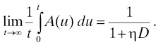
Define if the limit exists (and in all the models we study in this book, the limit does exist), and, as r∞ is just a number, we call it the asymptotic failure rate of the system reliability process. Again, r∞ ≥ 0.
For requirements pertaining to “failure rate,” be sure that all stakeholders interpret the phrase the same way. In particular, reliability engineers should advise the system engineer as to constancy of the “failure rate” in whatever model they use for the system reliability process.
Language tip: For a point process, “failure rate” as defined in item 1 is also referred to as “failure intensity.” This is particularly prevalent in the software reliability field. Consistently using “failure intensity” for the concept defined in item 1, above, avoids the use of “failure rate” altogether in any facet of reliability engineering or modeling. Some may consider this desirable, but it by no means universally accepted as a common practice even though a strong case could be made for it as a best practice because it avoids any confusion about the varying interpretations of “failure rate” that plague this field.
Modeling tip: Much of the reliability engineering community uses “failure rate” for the concept we have labeled “hazard rate” or “force of mortality” in Section 3.3.3.4. Note in fact that we are now dealing with a completely different situation, namely, the system reliability process model for a repairable system, rather than the single failure that can occur for a non-repairable system, as dealt with in Chapter 3. In a field that has numerous opportunities for confusion because of reuse of terms in different contexts, this is perhaps the most vexing. Ascher and Feingold [1] finesse this issue by avoiding “failure rate” altogether; for nonmaintained systems, they use the terminology “hazard rate” and “force of mortality” as we do, and for maintainable systems they use “rate of occurrence of failures (ROCOFs)” for “failure intensity” as defined in this section. Possibly, the best way to keep all this straight is to recall that to engineers, “rate” usually means “count per unit time” and that is what the definitions in the list given earlier encapsulate (use of the derivative means we are really looking at an “instantaneous” rate, as explained in elementary calculus, but it is an honest engineering interpretation of rate as usually understood). Be alert for this potential confusion whenever you encounter “failure rate.” In this book, whenever we use “failure rate,” it will always pertain to a maintainable system, and be defined as in item 1 in the above list. Item 2 will always be referred to as “asymptotic failure rate.”
Using the notation of Figure 4.1, the system failure rate refers to how rapidly the Sk are accruing on average. If the failure rate is small, the failure times tend to occur rather infrequently; while if the failure rate is large, the failure times tend to be denser on the time axis.
There are many system models in which the failure rate, as defined in item 1 of the above list, is not constant. One such, in very common use, is the revival model described in Section 4.4.3. In the revival model, the system failure rate (system failure intensity) may be decreasing, increasing, or variable. If the system failure rate is decreasing, then on average, failures are occurring less frequently and the times between outages tend to increase. If the system failure rate is increasing, then on average, failures are occurring more often and the times between outages tend to decrease. Ascher and Feingold [1] refer to the former as “happy systems” and the latter as “sad systems.” It is possible that the system failure rate may fluctuate, that is, be neither increasing nor decreasing throughout; models exhibiting this behavior are unusual in practice, but there is no theoretical reason why they cannot be used.
4.3.3.2 Operating times, times between outages, and times between failures
In Figure 4.1, the operating times are the intervals U1, U2, . . . ; during these time intervals, the system is operating without violation of any requirements (i.e., without any failures). The sequence U1, U2, . . . of operating time random variables constitutes a stochastic process.
Language tip: The operating time random variables are sometimes (usually!) called times between failures. This would be appropriate if we were to consider “failure” to refer to an entire outage interval instead of the instant at which the violation of a system requirement happens. This is the interpretation that commonly prevails even though it is an inconsistent use of terminology because a “failure” is something that takes place at a particular instant (the Sn in the system history diagram) whereas the “outage” is the period of time following a failure during which the failure condition (requirements violation(s)) persists. That the times between failures are in fact S2 – S1, S3 – S2, . . . has the perverse consequence that one may increase the times between failures by increasing the outage times while leaving the operating times alone. When you need to talk about the time periods during which the system operates properly, it is best to use the U1, U2, . . . as “operating times” or “times between outages.” See Exercise 1.
As they are random variables, we may consider the sequence of their expected values EU1, EU2, . . . . In some reliability models (see especially Section 4.4.2), these expected values are all the same. In such cases, it makes sense to define the mean time between outages as this common value. This is often (usually!) called the “mean time between failures.” Refer to the previous “Language tip” to clear up any ambiguity. In addition, specification of a single number for “mean time between outages” implies that there is a single mean time between outages, namely, that it is a constant. Be aware that many studies of repairable systems do not take pains to assure that this mean time between outages (MTBO) is a constant even though only a single number may be quoted. This is of some importance for systems engineers because a good grasp of potential system behaviors is required for effective design for reliability.
4.3.3.3 Outage times
In the system history diagram (Figure 4.1), the outage times are the intervals D1, D2, . . . ; during these time intervals, one or more system requirements are being violated (i.e., one or more system failures have taken place and have not yet been remediated). The sequence D1, D2, . . . of outage time random variables constitutes a stochastic process. As they are random variables, we may consider the sequence of their expected values ED1, ED2, . . . . In some reliability models, these expected values are all the same. In such cases, it makes sense to define the mean outage time as this common value.
4.3.3.4 Availability
Availability, denoted A(t), is an important concept and is widely used as a reliability figure of merit in requirements. A(t) is defined as the probability that the system reliability process is in the up state at time t. If we let Z(t) = 1 when the system is in the up state and Z(t) = 0 when the system is in the down state, then the stochastic process {Z(t): t ≥ 0} is the system reliability process. At each t, the value Z(t) is a reliability effectiveness criterion and its expected value A(t) = EZ(t) is called the system availability, or simply availability. When the system reliability process starts in the up state, A(0) = 1 and A(t) decreases from there. As a rule, in most systems of practical interest to systems engineers, availability will vary up and down for a while but eventually settle down to a limiting value (t → ∞) (further discussed in Sections 4.4.2 and 4.4.3); see also Refs. 12, 22. Methods for computing availability are discussed in Sections 4.4.2 and 4.4.3. In considering maintainability and supportability, special kinds of “availability” are defined by eliminating from consideration certain of the outage times that may stem from preventive maintenance, logistics delays, and other actions not having to do with correction of a failure. See Section 10.6.4.
It can be shown that the total time during the interval [0, t] that the system spends in the “up” state is given by
and the total time during [0, t] that the system spends in the “down” state is
from which it follows that the expected system downtime in [0, t] is given by
This vital connection was used in the example in Section 3.4.2.2.
Common practice distinguishes three different availability figures of merit, inherent, operational, and achieved availability. These differ in what components of outage times are counted in the downtime for each type. See Section 10.6.4 for the details (we have not yet discussed the corrective and preventive maintenance and supportability times that enter into these definitions).
4.3.4 When is a Maintainable System Not a Maintained System?
Up to now, we have used the words “maintained,” “maintainable,” and “repairable” interchangeably. There is one important case where we need to make a distinction, namely, where a maintainable system may have failure modes that cannot be corrected while it is in use. Consider a military aircraft. Such aircraft are used for “missions” of some duration, and commanders are vitally interested in the probability of successful mission completion (from many points of view, but these at least include no aircraft system failures during the mission). The important point is that there is no opportunity to repair some kinds of failures (especially hardware failures) during the mission, and while the aircraft is maintainable while on the ground, some kinds of corrective maintenance cannot be carried out while in flight. This does not preclude the possibility that some failures may be recoverable in flight. For example, a reboot of the affected subsystem may correct a software failure, and it may be possible to do this during flight if this capability has been provided in the system maintenance concept.
For such systems, a key reliability figure of merit is the probability that the system continues to operate properly for the entire duration of the mission. In this sense, techniques applicable to nonrepairable systems are used to say something about the probability of mission completion without failures because as far as the mission is concerned, the system is not repairable during the mission. In most cases, of course, the systems involved in the mission are not new at the start of the mission but may have already accumulated some age and can be described as some number of hours old at the start of the mission. The key variable of interest, then, is not the time to first failure of a brand new system, but rather the time to the next failure of a system (that may have already experienced many failures and repairs) that is a stated number of hours old at the start of the mission. This is the forward recurrence time from a stated age and will be discussed further in Sections 4.4.2 and 4.4.3.
4.4 MAINTAINED SYSTEM RELIABILITY MODELS
The most commonly used maintained system reliability models are the renewal model and the revival model. The words describe what kinds of repairs are performed to restore the system to functioning condition. These are discussed in detail in this section.
Many other maintained system reliability models are available in the literature. These are useful when more detailed modeling of special conditions is required. For example, the renewal model and the revival model do not account for the possibility that a repair person may introduce additional faults during the remediation of a failure (this is called the “clumsy repairman problem”). An example of a general model of this kind is given in Ref. 4. If you know that special conditions exist that are not part of the standard renewal or revival protocols, it is best to consult a reliability engineering specialist.
4.4.1 Types of Repair and Service Restoration Models
Whenever it is necessary to repair a system that has failed, some time is consumed. More descriptive system reliability models account specifically for these times, which is to say that the D1, D2, . . . intervals seen in the system history diagram are positive. This bears mention because some approximate system reliability models are used in which the outage times are assumed to be zero. In effect, this is an approximation that says that the outage times are so short compared to the operating times (times between outages) that making a model in which these are zero can provide a reasonable approximation for certain purposes (see Sections 4.4.2.1 and 4.4.3.1).
Modeling tip: In a model in which all the outage times are zero, the system availability is always 1 (because Z(t) = 1 except on a finite set of t-values). So such models are not appropriate where studies of availability and downtime are needed.
4.4.2 Systems with Renewal Repair
When a system is repaired according to a “renewal” protocol, it is returned to “good as new” condition after it fails and operation continues [2]. Most often, this means that the system is entirely replaced by a new one. This can be a costly strategy for large systems, but it is not unheard of. For example, weapons destroyed in battle may be replaced with new ones. Also, line-replaceable units (LRUs) in large, modular systems are often replaced with new ones when they fail (see Section 4.4.5.1 for coverage of this case).
4.4.2.1 Renewal models with instantaneous repair
In models in which the replacement by a new unit is assumed to consume no time, all the outage times in the system history diagram are zero. The resulting system reliability process {U1, U2, . . .} comprises a sequence of (necessarily nonnegative) stochastically independent, identically distributed operating times. The independence comes from an understanding that the length of time that a system has operated since its most recent failure has no influence on the length of time a replacement might operate: even though there may appear to be some correlation, we can’t see a cause-and-effect relationship (of course, if this is not true, we need to adopt another modeling condition). The identical distribution comes from the similarity of the replacement to the original unit: the failed unit is replaced by one of the same type. These assumptions produce a system reliability process known as a renewal process: a sequence of nonnegative (because they are lifetimes), independent, and identically distributed random variables [11]. Denote the common distribution of the Ui by F and let μ < ∞ denote its mean.2 The renewal process is a simple, well-understood process for which many results of interest to systems engineers are known.3 Some of these are
The expected number of renewals (failures, in the reliability model) in the time interval [t, t + h] is asymptotic to h/μ as t → ∞.
The expected number of renewals in [0, t], divided by t, approaches 1/μ as t → ∞. In reliability language, the asymptotic failure rate (Section 4.3.3.1) for the renewal process is 1/μ.
The asymptotic distribution of the forward recurrence time from time x is given by
as x → ∞. If we imagine x as the current time, the asymptotic distribution of the time to the next failure after x describes the forward recurrence time from a given time point (x) for a system that has been in operation for a long time. In practical terms, a “long time” generally can be safely interpreted as about 5 μ or greater.
Let N(t) = max{n : Sn ≤ t} denote the number of renewals in [0, t]. The expected number of renewals in [0, t], denoted by EN(t) = M(t), is given by the solution of the integral equation:
When F is exponential, F(t) = 1 − exp(−t/μ), then M(t) = t/μ for all t. Unfortunately, this equation has a closed-form solution for only a few other life distributions, but it is relatively easy to solve numerically [22]. The renewal process whose inter-renewal times are exponentially distributed is a homogeneous Poisson process with rate 1/μ [11].
The failure rate over the time interval [t, t + h], as defined in Section 4.3.3.1, for the renewal process is
Its expected value is h−1[M(t + h) − M(t)] which, for a renewal process whose inter-renewal time distribution has a finite mean μ, converges to 1/μ as t → ∞. By a slight abuse of terminology, it is often said that “the failure rate of a renewal process is 1/μ.” What is correct is that the expected asymptotic failure rate of a renewal process is 1/μ (the equality h−1[M(t + h) − M(t)] = 1/μ holds for the homogeneous Poisson process as well as for a stationary renewal process [11] but does not hold for any other renewal process when t < ∞). Consequently, you may need to verify the way “failure rate” may be used in this context.
4.4.2.2 Renewal models with time-consuming repair
A more realistic model is obtained if we allow the repair (or outage) times to be nonzero. In this case, the {Di} are a significant part of the model. Following the renewal paradigm, we assume that D1, D2, . . . are independent and identically distributed with common distribution G which has mean ν < ∞. The independence comes from a belief that there is no, or we can find no reason to suspect the existence of, mechanism that would cause an outage time to be influenced in any way by the outage times preceding it. The identical distribution comes from the idea that it is the same system that fails each time, so it is fair to describe the outage times for it as coming from a single population. Of course, these are idealizations and often ignore some facts that we may know or suspect to be relevant, so the model provides an approximation to reality that is more or less acceptable depending on the strength of the ignored facts. See Section 4.5 for some additional information.
The sequence {U1, D1, U2, D2, . . .} is called an alternating renewal process [11] because it consists of two renewal processes interleaved [12]. The system reliability process is the 0–1 process Z(t) = I{t falls into a U-interval}. The reliability model for a system with time-consuming renewal repair consists of information that can be derived from these assumptions.
The system availability (Section 4.3.3.4) is A(t) = P{Z(t) = 1}, the probability that the system is operating at time t. System availability is a reliability figure of merit. In the alternating renewal process model, assuming the system begins operation at time 0 in the operating state, we may write an integral equation for system availability as follows:
where H = F*G is the convolution of F and G (Section 3.4.5.2). The solution of this equation is given by
where MH is the renewal function (Section 4.4.2.1) for H. Again, closed-form solutions are rare, but numerical evaluation is straightforward [22]. The asymptotic availability is given by
which is the mean time between outages (mean operating time) divided by the mean cycle time (time from one failure to the next).
The number of system failures in [0, t] is given by N(t) = max{n : Sn + Un+1 ≤ t} with the convention that S0 = 0 and again assuming the system begins operation at time 0 in the operating state. The expected number of system failures in [0, t] when the system starts in the up state at time 0 is 1 − F(t) + MH(t).
The system failure rate over a time interval [t, t + h] is given by h−1[N(t + h) − N(t)], which has expected value h−1[MH(t + h) − MH(t)]. As t → ∞, this converges to 1/(μ + ν), the reciprocal of the mean cycle time. See the discussion of failure rate for the renewal process (Section 4.4.2.1).
Example: A fluorescent tube has the life distribution F(t) = where t is measured in hours. When the tube fails, it is replaced with a new one and the replacement time has a uniform distribution U2,6 on [2, 6], again with time measured in hours. What is the expected number of tube replacements per socket in 20 years of operation?
Solution: The conditions of the problem make it appropriate to use an alternating renewal process model to describe the system dynamics (by “system” here we mean the socket containing the tube, and by “dynamics” we mean the pattern of tube replacements in that socket). In the alternating renewal process model, the expected number of replacements in 20 years is the renewal function for F*U2, 6 evaluated at 175,320 hours (20 years). Numerical computation of this renewal function [22, 25] shows that F*U2,6(175,320) = 7.367. Absent the ability to carry out this numerical computation, we may reason that the average replacement time (4 hours) is so short compared to the average tube lifetime (23,305.6 hours) that the approximation afforded by a renewal process model (zero-duration replacement times) should be good. In that model, the solution is the renewal function for F evaluated at 175,320 hours. Numerical computation yields F(175,320) = 7.368. In this example, using the nonzero repair time model changes the result only in the third decimal place, a meaningless change in this scenario.4 Without the numerical computation, we may reason that 20 years is more than 5 mean tube lifetimes so that the asymptotic approximation shown in Section 4.4.2.1 may be used. The expected number of tube replacements in 20 years is then approximately 175,320/23,305.6 = 7.52, a slight overestimate of the true value. The availability in this system at 20 years is 0.999828728. The numerical computation shows that this value is reached at 12 years and remains steady (to this many decimal places) thereafter.
4.4.3 Systems with Revival Repair
The other most commonly used reliability model for repairable systems is the bad-as-old (BAO) model [1]. This model postulates that repair of a system is accomplished by returning it to operating condition without otherwise changing its age. That is, immediately after a repair, the system is working, but its age is the same as it was when it failed. The name BAO is intended to contrast with renewal repair that makes a system “good as new.” The BAO model provides a good approximation to the common scenario in which repair of a large, complex system is effected by replacing some part or subassembly that constitutes only a small part of the system. That small part of the system may be new (if the repair part is new) or of some other age (if the repair part comes from a spares pool of repaired items); but because it constitutes only a small part of the system, the overall age of the system (i.e., the accumulation of time against a clock measuring the time to the next failure) is not much changed. We abstract this (or approximate it) by saying that the change in age is, in the model, zero.
Example: Most automobile repairs are accomplished by replacing a faulty part with a new (e.g., voltage regulator) or rebuilt (e.g., alternator) one. In either case, the replaced part is only one of a great many failure-susceptible parts in the automobile. All the parts that were not replaced retain their age at the time of the failure of the replaced part, so the next failure is much more likely to come from one of the parts that were not replaced because there are so many more of them. So the time to the next failure is mostly unaffected by the replacement, and this is the postulate of the BAO or revival model. See Exercise 3.
To make further progress, we need to distinguish the case in which repairs are considered instantaneous from the case in which repairs are time-consuming.
4.4.3.1 Revival models with instantaneous repair
Mathematically, the BAO model says that the conditional distribution of the time to the next failure, given the occurrence time of the failure, is the same as the distribution of the time to the first failure. From the point of view of aging of the system, it is as if all the failures, up to and including the one taking place at Sn, had never happened. That is, applying this reasoning to the nth failure that takes place at time Sn, the model postulates that the conditional distribution of the time Un+1 to the next failure satisfies
for all n = 1, 2, . . ., where F is the distribution of U1. Thompson [21] shows that this property entails that the sequence of failure times {S1, S2, . . .} forms a Poisson process whose intensity function is given by the hazard rate of the distribution of U1. That is, if U1 ~ F and the hazard rate of F is h, then the number of failures in [0, t] has a Poisson distribution
where H is the cumulative hazard function . It is easy to show also that H(t) = −log[1 − F(t)] for t ≥ 0. From this, we can see that if F(t) = 1 − exp(−λt), then H(t) = λt and the process is homogeneous with constant intensity function λ. For every other life distribution F, the process is nonhomogeneous.
Language tip: (possibly the most important one in this book): The revival process with an exponentially distributed time to first failure is a homogeneous Poisson process because h(t) = λ and H(t) = λt. This is the source of a great deal of confusion in both the language and the modeling in reliability engineering. Foremost is that the failure rate (failure intensity) λ of the process is equal to the hazard rate (usually called “failure rate,” see Section 3.3.3.5) of the distribution of the time to the first failure. The simplest system reliability model is a single unit that has an exponential life distribution and is replaced upon failure by another of the same type. The process of replacement times in this case is both a renewal process and a homogeneous Poisson process having a constant failure rate. It is easy to overapply this simple model to situations where it does not apply. Many engineers mistakenly believe that this model is the beginning and end of reliability modeling. Even a cursory review of this chapter will show that this is far from accurate. Yet the language and modeling errors brought on by this point of view persist: all failure rates are constant, all times between outages have the same mean, availability is always equal to its asymptotic value, and many other such beliefs are common. Fortunately, increasingly capable reliability modeling software is beginning to make more complex reliability modeling readily accessible, and the persistence of these mistaken ideas should diminish. As a systems engineer, be aware that errors and oversimplifications are common in reliability modeling, and be prepared to ask for clarification where required. See also Section 4.4.6.
Example: A sonar system contains 16 individually replaceable beam-former units. When one beam-former fails, the system is inoperative. The beam-former lifetime has a gamma distribution (Section 3.3.4.7) with location parameter 44,350 hour−1 and shape parameter 2. The remainder of the system comprises power supplies, displays, signal processing units, antennas, and other essential equipment. When a beam-former fails, it is replaced by a working unit from an inventory of spares. The replacement process takes about an hour. What is the expected number of beam-former failures in the first 5 years of operation of the system?
Solution: We may use a revival process model for the sequence of failure times of the beam formers because when we replace a failed beam former, we are only affecting one-sixteenth of the ensemble. The approximation afforded by assuming that the replacement time is negligible compared to the mean operating time is good because the mean operating time is more than four orders of magnitude larger than the replacement time. So we may use the revival model with instantaneous repair for this scenario. The time to the first failure of the system we are considering (the ensemble of 16 beam formers, each of which is a single point of failure) has the survivor function
The mean beam-former life is 88700 hours = 10.12 years. For this survivor function, the cumulative hazard function is . Thus the sequence of beam-former failure times is approximately a (nonhomogeneous) Poisson process with intensity function H′(t). When t = 5 years = 43,830 hours, H(t) = 4.82. This is the expected number of individual beam-former failures, out of the group of 16 beam formers, in 5 years. See Exercise 4.
4.4.3.2 Revival models with time-consuming repair
So far, we have discussed the revival model only with zero repair times. The same reasons that we needed to consider time-consuming repair in the renewal model apply in the revival case as well. This aspect of the theory is not yet completely developed, however. We will review here what is known. The basic model begins with a nonhomogeneous Poisson process describing the operating times {U1, U2, . . .} of the unit being studied, so that repair of the unit is done according to the revival protocol. Each time a failure occurs, a repair is undertaken, and the repair times {D1, D2, . . .} form a renewal process with ED1 = D, 0 < D < ∞. This model is used when there is no reason to believe that the repair times depend on the index number of the failure being corrected. This is usually a reasonable assumption. We assume that the sequences of operating times and repair times are independent to reflect a belief that the length of time it takes to complete a repair has nothing to do with how long the unit was operating before it failed.
Denote by F the distribution of U1, the time to the first failure, and suppose F has a continuous density f and cumulative hazard function H = −log(1 − F). We further suppose that with 0 < η < ∞. With Sn = U1 + ⋅ ⋅ ⋅ + Un and NU(t) = min{n : Sn ≤ t}, it is shown in Ref. 24 that and so that the process {S1, S2, . . .} is tame [12].
Now let N(t) denote the number of failures in the revival process with nonzero repair times {U1, D1, U2, D2, . . .}. As a result of these preliminary considerations, the salient facts about the revival process with nonzero repairs times are
The asymptotic overall failure rate is
The asymptotic average availability is
Note that this expression is only for the asymptotic average availability. This is weaker than the corresponding result for alternating renewal processes. It is not yet known whether the stronger result can be established for the revival process with nonzero repair times.
It is also shown in Ref. 12 that the availability in the revival process with time-consuming repair can be computed by evaluating the integral
where and G is the common distribution of the downtimes. Unfortunately, this is not yet of much practical help because a satisfactory expression for EN(x) is not yet known.
Requirements tip: If the system has an availability requirement, and if the system can reasonably be modeled using the revival process with time-consuming repair, then demonstrating compliance with the availability requirement will be difficult until an expression for availability, rather than only the average availability over a long time interval, is developed. Usually, when an availability requirement like “The system availability shall not be less than 0.98. . .” is put in place, reliability modeling to asses compliance with the requirement uses the formula for asymptotic availability in an alternating renewal process (Section 4.4.2.2) to compare with the requirement. Even this does not completely cover the requirement because it is possible under not unusual conditions for the system availability to decrease below its asymptotic value, and even oscillate above and below. The asymptotic value alone does not reveal the transient behavior of availability. In case an alternating renewal model is appropriate, transient availability can be solved for by numerically solving the availability integral equation found in Section 4.4.2.2. This is less readily accomplished in the revival model with time-consuming repair: while the previous equation shows how to compute the transient availability in this model, the difficulty is transferred onto the computation of EN(t) in this model, and this is not yet a routinely solved problem. See Exercise 5.
Example: Consider the sonar system example in Section 4.4.3.1, but now the repair times are independent and identically distributed with a mean of 2 weeks (336 hours). What are the asymptotic overall failure rate and the asymptotic average availability of the beam-former ensemble?
Solution: We continue to use the revival model for beam-former replacement, but now we treat the repair times as nonnegligible. When we assumed instantaneous replacement, the expected number of beam-former replacements in 5 years is 4.82. Taking into account the nonzero repair times, we find that η = 16/α = 0.000361, D = 336, and the asymptotic overall failure rate is 0.000322. The asymptotic average availability is 0.89.
4.4.3.3 Approximations
The most prominent approximation used in reliability modeling for maintained systems is the one we have already discussed in Sections 4.4.2.1 and 4.4.3.1, which is that in most cases, typical operating times are so long compared to typical repair times that the repair times may be taken to be zero at least for the purpose of computing the failure rate. If an estimate of availability is required, this will not do, and a model that explicitly incorporates nonzero repair times will have to be used.
Other approximations have been proposed, including the method of phase-type distributions [13, 15] which approximates an arbitrary life distribution by a special distribution that is the distribution of the time until absorption in a Markov process with one absorbing state. This approximation permits the use of matrix methods and well-known linear algebra techniques to obtain numerical results for several useful reliability models [14]. Advancing capabilities in applied probability numerical computations have rendered these methods of more theoretical than practical interest, and this trend is likely to continue.
4.4.4 More-General Repair Models
In reality, the repair models we have described so far rarely capture perfectly everything we might know to be pertinent in a maintenance situation. The BAO or revival model when used to describe the replacement of a single failed component or subassembly in an ensemble of many components or subassemblies that are not replaced is not quite exact, yet it provides decent results in most cases in practice. But beyond the matter of model stability, some repair situations require more detailed treatment. One example is the case of the clumsy repairman. While repairing an item, even if the target failure is remedied, other faults that may later cause failures may be introduced inadvertently. This phenomenon is common enough in software projects that it has been studied extensively in the software engineering community [8, 9]. A general framework has been proposed [4] in which other important phenomenon like imperfect or incomplete repair may be introduced. Of course, the proper approach to this issue is to train staff so that erroneous repairs are avoided. The model is there to help with the inevitable occasional error that may occur even with highly trained staff.
As usual, the decision to employ more complicated models like these is guided by the amount of precision needed in the study. In all but the most critical cases, the approximations afforded by the commonly used models described earlier give acceptable results. For high-value and/or high-consequence systems, the need for additional precision may warrant the extra prevention cost that would be incurred to acquire or develop more specialized models. Use of higher precision models carries with it the obligation to use more precise information as input (life distribution estimates, etc.). Most routine reliability modeling is well-served by the approximations in common use because the quality of the input information usually available does not justify the use of extremely precise models. Indeed, the understanding of how component reliability estimate errors combine to produce errors in the reliability estimates (“predictions”) for higher level units and assemblies does not yet exist except for ensembles of single points of failure (series systems); see Section on “Confidence limits for the parameters of the life distribution of a series system.”
4.4.5 The Separate Maintenance Model
It is very common in defense systems, telecommunications systems, and other highly complex technological systems to find that the system maintenance concept involves correcting failures by replacing a failed subassembly with a working one drawn from a pool of spares. This is discussed further in Chapter 10. The separate maintenance model is convenient for creating a reliability model consistent with this maintenance concept.
Language tip: Beware of possible confusion in terminology: the separate maintenance model is a reliability model, intended to describe the reliability of a system that is maintained using the plan described earlier. In Chapter 11, we will consider a maintainability model based on the same maintenance plan. The goal of the maintainability model is to describe the number of maintenance actions taking place during some stated time interval.
To implement the separate maintenance model, arrange the system’s reliability block diagram so that there is a one-to-one correspondence between units (subassembly or subsystem) designated as replaceable in the system maintenance concept (Chapter 10) and blocks in the diagram. Then, write the structure function (Section 3.4.6) φR(X1, . . ., Xn) associated with this reliability block diagram. Denote by Z1(t), . . ., Zn(t) the reliability processes (Section 4.3.3.4) of the replaceable units or subassemblies5 of the system. The separate maintenance model is the reliability process Z(t) = φR(Z1(t), . . ., Zn(t)) of the ensemble of the replaceable units. Different separate maintenance models, all following this same general layout, are obtained when different descriptions of the individual LRU reliability processes Z1(t), . . ., Zn(t) are imposed.
Example: Consider a single server rack in a server farm. The rack contains 12 servers, a two-element hot-standby redundant power supply, a cooling fan assembly, a cabling harness, and a backplane. The 12 servers, each power supply, the cooling fan assembly, and the backplane are individually replaceable or serviceable. Backplane failures can occur because they often contain passive components, and connectors wear from insertion and reinsertion of circuit cards. All other elements of the rack (the rack frame and the cable harness) are permanent installations and their failure would require reconstruction of the rack; we will not include these failures in this model. Rack failure is defined as failure of any server, failure of the redundant power supply pair, failure of the cooling fan assembly, or failure of the backplane. In the hot-standby power supply arrangement, each power supply is individually replaceable. In order for the power supply pair to fail, one power supply would need to fail and the other would need to fail during the time the first supply is being replaced. Failure of one power supply puts the rack in a brink-of-failure state. Hot standby systems with individually replaceable units fail infrequently under normal circumstances. If it takes a positive amount of time to switch from a failed power supply to its redundant unit, that time must be accounted for in total rack outage time. If the power supplies are configured in a hot standby load-sharing arrangement, there is no switchover time. Backplanes are not generally replaceable but are repaired in place by removing and replacing individual components. This is generally a time-consuming activity: Telcordia GR-418 [20] specifies a mean time to repair of 48 hours for backplanes.
Label the servers 1–12, the two power supplies 13 and 14, the fan assembly 15, and the backplane 16. Then a reliability block diagram for this rack is shown in Figure 4.2.
Figure 4.2Server rack example reliability block diagram.
The structure function associated with this diagram is
Label the reliability process for the servers as R(t), that for the power supplies P(t), that for the fan assembly F(t), and that for the backplane B(t). Then the reliability process for the rack is
Here, we have assumed that all the servers have the same reliability characteristics and both power supplies have the same reliability characteristics. If this is not true, the labels will have to be redefined accordingly. Modeling continues by selecting a repairable system model for each of R, F, B, and P from those described in Sections 4.4.2 and 4.4.3, or some other source. See Sections 4.4.5.1 and 4.4.5.2.
For availability in the separate maintenance model, let A1(t), . . ., An(t) denote the availabilities for each of the reliability processes Z1(t), . . ., Zn(t). Then the system availability is given by A(t) = φR(Z1(t), . . ., Zn(t)) [3]. Computing the number of failures or failure rate for the separate maintenance model is more complicated. The details may be found in Ref. 23.
4.4.5.1 Separate maintenance with renewal lru replacement
The separate maintenance model can be used with any reliability process (Section 4.3.2) description for each of its components. Not all components need have the same reliability process description. In this section, we study the separate maintenance model when the individual component reliability processes are renewal or alternating renewal processes.
Consider a system whose structure function is φR(x1, . . ., xk). The individual component reliability processes are alternating renewal processes (Section 4.4.2.2) Z1(t), . . ., Zk(t) whose availabilities are denoted by A1(t), . . ., Ak(t), respectively. Then the system availability is given by φR(A1(t), . . ., Ak(t)) [3]. If the mean operating time and mean outage time for component i are μi and νi, respectively, for i = 1, . . ., k, then the asymptotic system availability is given by
If the entire system consists only of single points of failure (i.e., is a series system), then the number of system failures is N1(t) + ⋅ ⋅ ⋅ + Nk(t) where Ni(t) is the number of failures in time t in alternating renewal process i, i = 1, . . ., k. The expected number of failures and availability for each individual component reliability process may be computed using the expressions given in Section 4.4.2.2. If the system is not a series system, the system availability is still given by φR(A1(t), . . ., Ak(t)), but computation of the number of system failures is more complicated. The method is outlined in Ref. 23. For a parallel (hot standby) system comprising m units whose structure function is given by φR(x1, . . ., xm) = 1 − (1 − x1) ⋅ ⋅ ⋅ (1 − xm), the expected number of system failures in [0, t] is given by
where A(t) = 1 − (1 − A1(t)) ⋅ ⋅ ⋅ (1 − Am(t)), Fi and Gi are the operating time and outage time distributions for unit i, Hi = Fi*Gi, and is the renewal function (Section 4.4.2.1) for Hi, i = 1, . . ., m (equation (4.10) of Ref. 23).
When the reliability process descriptions are renewal processes (zero outage times), the system availability is always 1. Counting the number of system failures is again accomplished by the method outlined in Ref. 23 but now Hi = Fi.
Example: Return to the server rack example shown in Figure 4.2. We will determine the mean and standard deviation of the time to the first rack failure and the expected number of maintenance actions, availability, and cumulative expected downtime for the rack under the separate maintenance model with renewal repair. To do this, we need to know the operating time and outage time distributions for each of the rack’s components. These are as given in Table 4.1.
Gamma, mean 40,000 hours, standard deviation 15,000 hours
Lognormal, median 6 hours, shape factor 2
Power supply
Weibull, α = 2,000, β = 1.4
Lognormal, median 6 hours, shape factor 2
Fan
Exponential, mean = 105 hours
Lognormal, median 6 hours, shape factor 2
Cable harness
Exponential, mean = 106 hours
Lognormal, median 6 hours, shape factor 2
Backplane
Exponential, mean = 5 × 10⁵ hours
Lognormal, median 168 hours, shape factor 1.8
The mean time to the first rack failure is 2481.9 hours, and its standard deviation is 1345.1 hours. Over the first 40,000 hours of operation (~5 years), the cumulative expected number of rack failures is shown in Figure 4.3, the availability is shown in Figure 4.4, and the cumulative expected downtime is shown in Figure 4.5.
At the end of the study period, 40,000 hours, the cumulative expected number of failures is 15.76, the availability is 0.97695, and cumulative expected downtime is 496.42 hours. It appears that the limiting value of availability has not yet been attained by the end of the study period. The minimum availability over the study period is 0.9766 (note the expanded vertical scale in Figure 4.4). To satisfy an availability requirement, it may be enough to show that the minimum value of availability is greater than the requirement. Numerical computations are again from Refs. 22, 25.
4.4.5.2 Separate maintenance with revival lru replacement
We now consider the case where Z1(t), . . ., Zk(t) are revival processes with zero repair times or revival processes with nonzero repair times. If repairs are instantaneous, the system availability is always 1 and the expected number of system failures for a series system is
where Fi is the distribution of the time to the first failure for component i, i = 1, . . ., m. An expression for the expected number of system failures for systems other than series systems is not known at this time.
When repair times are nonzero, little can yet be said because results relating the asymptotic average failure rate and asymptotic average availability for the system to the asymptotic average failure rates and asymptotic average availabilities for its components remain to be developed.
4.4.5.3 Separate maintenance with a spares pool of repaired lrus
In a remove-and-replace maintenance concept with repair of failed LRUs, neither of the above two models is quite correct because replacement LRUs come from a spares pool that contains not only new LRUs but also LRUs that have previously failed and been repaired. If we assume repair of an LRU is accomplished by a renewal procedure, this is tantamount to assuming that all LRUs are new, and the model of Section 4.4.5.1 applies. However, realistic repair of an LRU is usually accomplished by replacing one or a few components on the LRU that had failed, and this is more appropriately described by a revival model (Section 4.4.3). After some period of operation, spares in the pool will have failed and been repaired perhaps several times, and a spare drawn at random from the pool will have a lifetime whose distribution is the same as the distribution of the length of the ith interval in a nonhomogeneous Poisson process for some (unknown) i. The number of times an LRU has been used previously should not decrease as time passes, but beyond that it is a complicated function of the maintenance concept’s dynamics. Solution of this challenging research problem would be useful in developing greater understanding of system reliability when the remove-and-replace maintenance concept is used.
4.4.6 Superpositions of Point Processes and Systems with Many Single Points of Failure
Consider a system containing N replaceable units, each of which is a single point of failure. In this system, there are no redundant units (or this could be a maintainability block diagram (Section 11.3.1) by which maintenance actions are being counted). Associated with each individual replaceable unit is a sequence of times at which failures of that unit occur. This sequence is an example of a point process, a stochastic process that has a continuous parameter space (here, time) and a discrete state space (here, number of failures). Because each replaceable unit is a single point of failure in this system, every time one of these units fails, the system fails. The sequence of failure times of the system is then the pool or superposition of the N sequences of failures times of the individual replaceable units. We may picture a superposition of point processes like this:
In Figure 4.6, the pool or superposition process is shown containing nine points over the time interval depicted. Three of these come from unit 1, two from unit 2, one from unit N, and three come from unspecified units (between 3 and N − 1) not shown in the picture. Note that each time a point appears in one of the unit failure time point processes, that same time point appears in the pool. The superposition is also a point process, and its intensity (Section 4.3.3.1) is the sum of the intensities of the pool’s constituent processes.
Figure 4.6Generic superposition of point processes.
Superpositions are useful in reliability modeling because of two relevant applications and one invariance property. One way that a superposition can arise is as the set of times at which system failures occur in a system containing only single points of failure, that is, series systems. Each time one of the system’s constituent units fails, the system fails, and the superposition of the individual unit failure time sequences is the system failure time sequence. Another way a superposition can arise is as the collection of times at which failures occur in a population of systems that is being tracked as part of data collection and analysis. Each time a failure occurs in one of the systems in the population, the count in the superposition process that describes the failure times of the members of the whole population increases by one. The invariance property is that under conditions that are usually satisfied in practice, the superposition of a large number of (independent and uniformly sparse) point processes becomes approximately a Poisson process as the number of constituent processes grows without bound. It is called an invariance principle because it doesn’t matter what the characteristics of the constituent point processes are—as long as there is no one (or some finite number of) processes that are so fast that almost all the points in the superposition come from those processes (this is roughly what is meant by “uniformly sparse”) and they are mutually stochastically independent.
The formal statement of this invariance property is called Grigelionis’s theorem [10]. It is a generalization of the easy-to-demonstrate property that the superposition of a finite number of independent Poisson processes (homogeneous or not) is also a Poisson process [11] (see Exercise 6). So a superposition is easier to deal with because it can be treated as a Poisson process in most applications.6 This fact may account for the common practice of treating the times between outages of a large system, or the times at which failures occur in a large population of systems being tracked, as though they had an exponential distribution. That is, the results of reliability modeling for some system may show that it has some life distribution. The invariance principle says that if the population of those systems being tracked is large enough, then failures will arrive in that population approximately according to a Poisson process regardless what the individual system life distribution was. Using this reasoning, it is possible to claim that you may as well make the system life distribution be as simple as possible, that is, exponential, but while this may not be inappropriate for collection of data from a large population of these systems, it may obscure needed information, such as availability, about the individual system.
4.4.7 State Diagram Reliability Models
We have so far discussed so-called structural reliability models based on the reliability block diagram and the life distributions of the diagram’s elements. These models are particularly suitable for the kind of system maintenance concept, often encountered in defense, telecommunication, and other large-scale systems, in which certain subassemblies of the system are designated as replaceable and remediation of a system failure is accomplished by replacing one or more of these subassemblies (the “remove-and-replace” maintenance concept). The separate maintenance model matches this operation well. However, there are other types of system maintenance plans and system operations for which the separate maintenance model is less well adapted. For these systems, an alternative reliability modeling strategy based on state diagrams can be useful.
A state diagram is a graph in which the nodes represent system states and the links represent transitions from state to state. If we number the states from 1 to N and let X(t) denote the state that the system is in at time t, then it is possible to posit conditions that make {X(t) : t ≥ 0} a Markov process. Among other things, this will mean that the sojourn time in each state (i.e., the time the system spends in each state) will have an exponential distribution, and the transitions from state to state are governed by a mechanism for which the probability of transition to another state depends only on the state the system is currently in and does not depend in any way on previously visited states. A Markov process of this type is an example of a continuous-time Markov chain (CTMC), a Markov process having a continuum parameter space (time) and a discrete state space.
Example: Let us describe the three-unit hot-standby redundant system with a state diagram. Label the units 1, 2, and 3. In Figure 4.7, a bubble containing some numbers indicates a system state in which the units numbered in the bubble are operating. A unit whose number does not appear in the bubble is failed (in that system state).
Figure 4.7State diagram for three-unit hot-standby redundant system.
In the state represented by the empty bubble at the bottom of the diagram, no units are operating, and this is the state in which the system (the three-unit hot standby ensemble) is failed. In all other states, at least one unit is operating, and thus the system is operating when it is in any of those states. The same diagram can also be used to describe the reliability of a three-unit series system. The states and transitions are the same, but the only state in which the system is not failed is the one labeled “1, 2, 3” at the top of the diagram.
It would appear that this method for modeling the reliability of the three-unit hot standby arrangement is more complicated than the structural method discussed in Section 3.3.4.5, and it has the additional disadvantage that the sojourn time (time spent in a state) distributions must all be exponential, so this would not be a good choice for modeling the reliability of the three-unit hot standby ensemble. It is also apparent that the number of states required for a state-diagram model of any system of substantial size is extremely, perhaps unmanageably, large. However, for more complicated systems, such as system operations involving queueing for repair, queueing networks, etc., where the structural approach is too complicated to use effectively, the state diagram approach provides a better (if not the only) alternative. A more comprehensive examination of factors to consider when choosing whether to use a separate maintenance model or a state diagram model for reliability is found in Ref. 25. Many treatments of the use of the state diagram approach in reliability modeling are available (see Refs. 16, 26 and others).
Yet other reliability modeling approaches are available. While citing the stochastic Petri net model [19] as another approach that is particularly suitable when the sequence (chronological order) of system operations influences its reliability, we make no pretense here to a thorough review of all possible models. An older review that is nonetheless helpful is Ref. 17.
4.5 STABILITY OF RELIABILITY MODELS
George Box has said “All models are wrong, but some are useful” [6]. This idea speaks to the impossibility of incorporating into a model all the factors that are known to be at play. Generally, the modeler’s judgment is the most important determinant of which factors will be included and which ignored. Consequently, every model of the type discussed in this chapter is at best an approximation and at worst mistaken, misleading, and dangerous. Systems engineers are perhaps the best suited by training and experience to sort out which is which in situations where time is short and information is sparse. However, there are mathematical results that give sufficient conditions for a model to have certain desirable properties, such as continuous dependence on the initial conditions of the problem. In high-consequence systems embodying mission criticality, economic make-or-break situations, or life-and-death safety situations, incorporating a formal study of reliability model stability may be worth the resources expended to assure that conclusions drawn from the models are supported with a degree of knowledge consistent with the seriousness of the scenario. A full treatment of these ideas is beyond the scope of this book, but one important point falling into this general area deserves mention. While the decision to adopt a more detailed reliability model depends to a great deal on the customer’s need for precision, it also depends on the precision of the information available as input to the model. This includes reliability estimates of the components and subassemblies making up the system. As discussed in Section on “Confidence limits for the parameters of the life distribution of a series system,” it is possible to aggregate precision information from components to form precision information for a series system, but how to do this for other structures remains an open problem. Nevertheless, it is fair to say that larger standard errors in the estimates of component reliabilities should lead to a larger standard error in the reliability estimate for any coherent structure containing those components.7 So if component reliability estimates are quite uncertain, then it may not be justifiable to use a very detailed system reliability model.
While it does not deal with reliability models specifically, the authoritative treatment of stability in stochastic models is [18].
4.6 SOFTWARE RESOURCES
Time was when reliability models of the sort described in this chapter had to be built from scratch and by hand for every new application. More recently, much of this knowledge has become commoditized and several vendors offer system reliability modeling software for either the separate maintenance model or the state diagram model approach. It is not the purpose of this book to recommend any software product or vendor over any other. Rather, your choice of software should be guided by the learning found in this chapter. Some questions to consider when choosing software include
Does the software offer a variety of life distribution options?
Does the software contain appropriate adjustments for environmental stresses?
Do you need to see confidence interval information for series system models?
Do the assumptions of the separate maintenance model or the state diagram model fit better with your understanding of system operation?
Does the software offer sensitivity analysis capability and/or reliability importance computations so that you can see how possible errors in component reliability specifications may be reflected in the system reliability model?
Does the software offer any reliability optimization models that may be useful in reliability budgeting (Section 4.7.3)?
Software is also available for other reliability engineering tasks, including fault tree analysis and failure modes, effects, and criticality analysis (Chapter 6), analysis of reliability data (including data from life testing and data from operation of installed systems) (Chapter 5). In addition, simulation can be a very effective tool for reliability modeling in complicated situations.
4.7 RELIABILITY MODELING BEST PRACTICES FOR SYSTEMS ENGINEERS
So far, Chapters 3 and 4 have introduced several reliability modeling tools that are useful for systems engineers to understand as part of the process of setting and evaluating the suitability of reliability requirements. How should these tools be put to use in the systems engineering process? Or, how should systems engineers direct the reliability engineering function for maximum added value to the product or service? In this section, we provide four perspectives on these questions.
4.7.1 Develop and Use a Reliability Model
The major purposes of the reliability modeling that have been discussed at some length in this chapter are
to assess the potential reliability of the design at any stage and to compare the reliability of alternative design proposals,
to check whether design for reliability activities have been successful in the sense that they have resulted in a system that has the potential to meet its reliability requirements,
to provide guidance for the data analysis needed for determining whether systems in operation do meet their reliability requirements.
The statistical analyses needed for these activities are described in Chapter 5. In all cases, we aim for the result of reliability modeling to be expressed in the same terms that will be used in the data analysis. That is, if the data to be collected are outage durations, times between outages (operating times), number of failures per stated time interval, etc., then a reliability model should be chosen that will produce as its output some information about outage durations, times between outages (operating times), number of failures per stated time interval, etc. These are reliability effectiveness criteria, and are as such random variables, so the output of the reliability model will necessarily be some abbreviation or summary of the reliability effectiveness criterion, that is, a reliability figure of merit. When comparing a reliability model with reliability requirements or with reliability data, arrange the data analysis so that the same reliability figure of merit appears on both sides of the comparison. For example, if a reliability requirement involves expected outage duration, then both the reliability model and the data analysis should address expected outage duration. Discussion of data analysis for both reliability effectiveness criteria and reliability figures of merit is found in Chapter 5 as well as in some examples in other chapters.
4.7.2 Develop the Reliability–Profitability Curve
The costs of reliability to the supplier include
prevention costs,
appraisal costs, and
external failure costs.
Prevention costs include everything the supplier does to influence the reliability of the product or service. These include developing reliability requirements and reliability engineering activities including reliability modeling and design for reliability. Appraisal costs include the cost of any reliability testing that may be performed during development as well as the portion of failure reporting, analysis and corrective action system or FRACAS (Section 5.6) operating costs attributable to the product. External failure costs include a tangible component (the cost of servicing any warranty that may be offered) and an intangible component (loss of potential sales because customer perception of the product’s reliability is poor). The cost of warranty servicing is direct, easily understood, may be offset by the sale of extended warranties, and immediately comprehensible to executives. The cost of loss of reputation is more difficult to pin down precisely, as it represents more abstract items like loss of business from potential customers who may be discouraged from purchasing from the supplier because the supplier’s reputation may have suffered from previously selling products with poor reliability.
Formal methods may be used to determine an appropriate balance between cost of reliability and expected profitability, but this is rare. Contemporary quality engineering principles support putting more resources into prevention with the goal of driving down failure costs to a far greater degree (the “1–10–100 rule”). Even if the reliability—profitability balance is addressed only informally, and the results are not very precise, there is value in the exercise because answers may be quite different for different classes of products. For example, it is likely that prevention costs will represent a higher proportion of development costs for an airplane, with its long useful life and high reliability needs, than for a consumer entertainment product which may rapidly become obsolete.
4.7.2.1 Warranty cost modeling
A typical warranty offered by a supplier contains conditions like: the supplier will repair or replace an item that fails when in use by the customer, for some period of time after the initial purchase. Projecting the likely cost of various warranty schemes is an important part of the planning a supplier must do to determine the likely profitability of a product or service. Detailed examination of warranty cost models is outside the scope of this book. The reliability engineering literature contains many studies of this kind; Blischke and Murthy [5] provide a good introduction. Because warranties are usually specified in terms of calendar time, the relationship between operational and calendar time is important for warranty modeling. See Sections 3.3.7 and 9.3.3.
4.7.3 Budget for Reliability
A complex system contains many components, subassemblies, and subsystems that may “fail,” that is, behave in such a way as to cause system failure (requirements violations). When reliability requirements are defined for a complex system, it is necessary to determine how the frequency and duration of component, subassembly, and subsystem failures and outages may be arranged so that the frequency and duration of system failures and outages satisfies the system reliability requirements. The process of parceling out the system reliability requirements to the components, subassemblies, and subsystems is called reliability budgeting. The goal of reliability budgeting is to assign to each component, subassembly, and/or subsystem a reliability characterization—probability of failure, life distribution, reliability process, etc., as appropriate—in such a way that
the system reliability requirements are met,
cost is minimized, and
the component/subassembly/subsystem can be designed to meet that target.
The formalism of reliability budgeting is mathematical programming or optimization. We can ask for an assignment of reliability to components, subassemblies, and subsystems to meet the system reliability requirements; or, if a fixed budget is given, we can ask to maximize the system reliability subject to the cost constraint implied by the budget. Either of these is a type of system reliability budget. An introduction to these ideas is found in Section 2.8.4.
For systems describable by the formalism developed in Sections 2.8.4 or 4.3, the system reliability budget begins with a reliability block diagram and its associated structure function. Many formulations of the reliability budget problem are possible, depending on the system reliability requirements. Here are a few examples, all for systems having a structure function φR and components whose reliability indicator functions are C1, . . ., Cn and whose costs are a1, . . ., an:
A nonrepairable system with a mission time requirement: In this case, the system survivor function is required to be at least as large as a given value s at a specified time T. If the component/subassembly/subsystem survivor functions are S1(t), . . ., Sn(t) having parameters λ1, . . ., λn, respectively (these may be vectors), then we may formulate the reliability budget problem for this system as
A repairable system with an availability requirement: In this case, the system availability is required to be at least as large as a given value α over a specified time interval [0, T]. If the component/subassembly/subsystem availability functions are A1(t), . . ., An(t), then we may formulate the reliability budget problem for this system as
Formulating the budgeting problem as an optimization problem is one thing, getting to a solution is quite another.8 This is not because the mathematics is complicated or beyond current capabilities. Rather, it is because of the difficulty in acquiring reliable information about the component/subassembly/subsystem costs as functions of their reliability or availability. A related difficulty is that there is usually not a continuum of choices for the components/subassemblies/subsystems as a function of their reliability or availability. It is usually not possible to marginally increase the reliability of a component by spending an additional cent on it. There may be only one or two choices for a component. This does not adversely affect the solution procedure—it is easy to write the cost function of such a component as a step function—but the greater practical difficulty is that this information is hard to come by and is usually so imprecise that making the effort to solve the budget problem formally is not justified by the quality of the information being used to feed it. In many cases, budgets are devised informally, and often this is “good enough” because the input information is so diffuse. Regardless, a reliability budget is necessary to proceed with design for reliability and creation of a budget, by whatever means, is a best practice.
4.7.4 Design for Reliability
Once you know what the reliability requirement for each component, subassembly, and/or subsystem is, you can begin to apply the design for reliability ideas found in Chapter 6. Best practice indicates that design for reliability is preferable to other reliability management practices inasmuch as design for reliability attempts to be proactive, uses lessons learned from prior experience, and is consistent with contemporary quality engineering principles.
4.8 CHAPTER SUMMARY
This chapter has provided background material on reliability modeling for maintainable systems that systems engineers need in order to be good customers and suppliers in the development process. It is possible to use this chapter as a framework for advanced study of reliability modeling, but its primary intent is to equip systems engineers to be effective in dealing with the reliability engineering aspects of product and service development.
The chapter covers reliability effectiveness criteria and reliability figures of merit used for maintainable systems. Those in most common use are times between outages, failure intensity (failure rate), and availability. Several types of repair models are covered.
We again caution extra care around “failure rate.” The phrase is used for several different concepts, some of which require special conditions, so you need to be aware of which meaning is intended in any particular case.
4.9 EXERCISES
A maintained system in operation yielded the following data: U1 = 28, D1 = 3, U2 = 50, D2 = 8, U3 = 17.6, D3 = 2, U4 = 33.9, D4 = 4.5, U5 = 71, D5 = 2.7, U6 = 108, D6 = 11, and at this point data collection ceased.
What is the total time of operation covered by this data collection?
Estimate the mean time between failures of this system over this period of operation.
Estimate the mean time between outages of this system over this period of operation.
Explain any differences you see.
Show that a system whose life distribution has an increasing hazard rate and which is repaired according to the revival protocol has an increasing failure rate. What can be said about this system if it is repaired according to the renewal protocol?
Suppose a system contains 1000 single-point-of-failure components, each of which has an exponential life distribution with parameters (mean lifetimes) λ1, . . ., λ1,000.
What is the life distribution of the system?
What is the mean life of the system?
Suppose component 1 fails at time T and is replaced instantaneously by a new one of the same type. What is the distribution of the time to the next failure after T? What is its mean?
Work the same problem with the life distributions of the components being Weibull with parameters (λ1, β1), . . ., (λ1000, β1,000).
Consider the example in Section 4.4.3.1. Suppose instead that each beam former is replaced by a new one when it fails and that the replacement time is negligible compared to the expected life of one beam former. Discuss the use of a superposition-of-renewal-processes model for this scenario. (Hint: you may also wish to consult Section 4.4.6.)
*From Section 4.4.3.2, find the expected value of N(x), the number of failures in the time interval [0, x]. Develop an expression for EN(x) so that the integral formula for availability may become useful. Hint: N(x) = max{n : Sn + D1 + ⋅ ⋅ ⋅ + Dn−1 ≤ x} and condition on the distribution of D1 + ⋅ ⋅ ⋅ + Dn−1.
Let Ni(t) be a Poisson process with intensity function λi(t), i = 1, 2. Suppose that the two processes are mutually stochastically independent. Show that the superposition of N1(t) and N2(t) is a Poisson process with intensity function λ1(t) + λ2(t). Hint: the superposition can be written as N1(t) + N2(t).
Consider a system composed of three units A, B, and C. A and B are in a hot standby redundant arrangement, and C is in series with this ensemble.
Draw a reliability block diagram for this system.
Write a structure function for the diagram.
Suppose the operating probabilities are pA, pB, and pC, and that the cost of each unit is proportional to (1/p) − 1 (p = pA, pB, pC). Suppose further that the system reliability is to be at least 0.99. Determine the values of pA, pB, and pC that meet the system reliability requirement at minimal cost.
Suppose the units have survivor functions Si(t) = 1 − exp(−λit), i = A, B, C, and that the system reliability requirement is that it survive for 10,000 hours with probability at least 0.99. Determine the values of λA, λB, and λC that meet the system reliability requirement at minimal cost.
*Suppose now that A, B, and C are repairable, all have repair time distributions that are uniform on [1, 4], and that the system availability requirement is 0.99 or better. Determine the values of λA, λB, and λC that meet the system reliability requirement at minimal cost.
*Suppose that A and B are a cold standby arrangement instead of hot standby. How does your solution change?
Consider the server rack example in Section 4.4.5. How would the analysis change if the power supplies were in a cold standby configuration?
REFERENCES
1. Ascher H, Feingold H. Repairable Systems Reliability: Modeling, Inference, Misconceptions, and their Causes
. New York: Marcel Dekker; 1984.
2. Barlow RE, Proschan F. Statistical Theory of Reliability and Life Testing: Probability Models
. New York: Holt, Rinehart, and Winston; 1975.
3. Baxter LA. Availability measures for a two-state system. J Appl Probab 1981;18:227–235.
4. Baxter LA, Kijima M, Tortorella M. A point process model for the reliability of a maintained system subject to general repair. Commun Stat Stoch Models 1996;12 (1):12–19.
5. Blischke WR, Murthy DNP. Warranty Cost Analysis
. New York: John Wiley & Sons, Inc; 1994.
6. Box GEP, Draper NR. Model-Building and Response Surfaces
. New York: John Wiley & Sons, Inc; 1987.
7. Cox DR, Isham V. Point Processes
. Boca Raton: CRC Press; 1980.
8. Fakhre-Zakeri I, Slud E. Mixture models for reliability of software with imperfect debugging: identifiability of parameters. IEEE Trans Reliab 1995;44 (1):104–113.
9. Gokhale SS, Philip T, Marinos PN. A non-homogeneous Markov software reliability model with imperfect repair. Computer Performance and Dependability Symposium, 1996, Proceedings of IEEE International; 1996. p 262–270.
10. Grigelionis B. On the convergence of sums of random step processes to a Poisson process. Theory Probab Appl 1963;8 (2):177–182.
11. Karlin S, Taylor HM. A First Course in Stochastic Processes
. 2nd ed. New York: Academic Press; 1975.
12. Marlow NA, Tortorella M. Some general characteristics of two-state reliability models for maintained systems. J Appl Probab 1995;32:805–820.
13. Neuts MF. Probability distributions of phase type. Liber Amicorum Prof Emeritus H. Florin 1975;173:206ff.
14. Neuts MF, Meier KS. On the use of phase type distributions in reliability modelling of systems with two components. Oper Res Spectr 1981;2 (4):227–234.
15. Neuts MF, Pérez-Ocón R, Torres-Castro I. Repairable models with operating and repair times governed by phase type distributions. Adv Appl Probab 2000;32:468–479.
16. Osaki S. Stochastic System Reliability Modeling
. Singapore: World Scientific; 1985.
17. Osaki S, Nakagawa T. Bibliography for reliability and availability of stochastic systems. IEEE Trans Reliab 1976;25 (4):284–287.
18. Rachev ST. Probability Metrics and the Stability of Stochastic Models
. New York: John Wiley & Sons, Inc; 1991.
19. Sahner RA, Trivedi KS, Puliato A. Performance and Reliability Analysis of Computer Systems
. Dordrecht: Kluwer Academic Publishers; 1996.
21. Thompson WA. On the foundations of reliability. Technometrics 1981;23 (1):1–13.
22. Tortorella M. Numerical solutions of renewal-type integral equations. INFORMS J Comput 2005;17 (1):66–74.
23. Tortorella M. On cumulative jump random variables. Annal Oper Res 2013;206 (1):485–500.
24. Tortorella M. Strong and weak minimal repair and the revival process model for maintained system reliability. 2014.
25. Tortorella M, Frakes WB. A computer implementation of the separate maintenance model for complex-system reliability. Qual Reliab Eng Int 2006;22 (7):757–770.
26. Trivedi KS. Probability and Statistics with Reliability, Queueing, and Computer Science Applications
. Hoboken: John Wiley & Sons, Inc; 2008.

if the limit exists (and in all the models we study in this book, the limit does exist), and, as r∞ is just a number, we call it the asymptotic failure rate of the system reliability process. Again, r∞ ≥ 0.

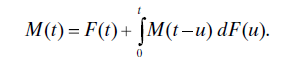
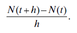
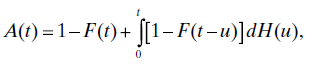
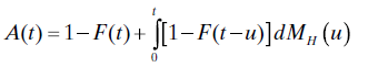
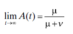
where t is measured in hours. When the tube fails, it is replaced with a new one and the replacement time has a uniform distribution U2,6 on [2, 6], again with time measured in hours. What is the expected number of tube replacements per socket in 20 years of operation?


. Thus the sequence of beam-former failure times is approximately a (nonhomogeneous) Poisson process with intensity function H′(t). When t = 5 years = 43,830 hours, H(t) = 4.82. This is the expected number of individual beam-former failures, out of the group of 16 beam formers, in 5 years. See Exercise 4.