
13
Design for Supportability
13.1 WHAT TO EXPECT FROM THIS CHAPTER
The material we present in this chapter supports execution of the prescription we consistently advocate: pay attention to sustainability engineering at the early stages of system design so that better results may be achieved at lower cost. Good supportability promotes customer satisfaction and supplier profitability by decreasing the amount of time it takes to recover from failures, decreasing the burden on maintenance staff, and increasing system availability. Some important factors influencing supportability were reviewed in Section 12.2.2. This chapter discusses several useful practices that provide a quantitative foundation for enhancing supportability. These practical techniques form the core of design for supportability. Many of these quantitative techniques may also be extended to optimize their application. The decision whether to take the extra time and resources to carry out this optimization rests, as usual, on a balance of prevention and external failure costs.
Coverage of modeling and optimization for all relevant supportability techniques is beyond the scope of this book, but we use this chapter to show how some important supportability issues may be addressed with quantitative modeling. As always, the depth to which techniques like these are applied is dictated by the economics of the system and its total life cycle cost picture. Products that become obsolete very quickly, are low value, or otherwise economically less consequential may receive less supportability attention, and some of the ideas in this chapter may be incorporated informally or possibly not at all. However, for expensive, complex, high-value, or high-consequence systems, the quantitative techniques introduced here are valuable in getting optimized supportability built into the system effectively. High-value and high-consequence systems justify more prevention cost and additional resources expended on design for supportability. Techniques presented here are not meant to be all-encompassing but rather are meant to provide an introduction to the thought process used in dealing with supportability needs quantitatively. It is unlikely that you will find a model here that exactly matches your situation. Rather, the models should serve as a source of ideas that may be adaptable to your needs. More complex models tailorable to more comprehensive needs, as well as models for other supportability practices not covered in this chapter, are available in the literature. The exercises also offer some practice in building quantitative models for supportability practices.
13.2 SUPPORTABILITY ASSESSMENT
13.2.1 Quantitative Supportability Assessment
As with reliability, it is useful for product and service designers to have a way to determine the supportability of the design as it progresses. Supportability is many-faceted, so different assessment models are needed for different facets. Aspects of supportability that lend themselves to quantitative modeling include
- inventory management for spare parts, repair parts, and consumables,
- logistics management for the transportation of required goods around the various locations specified in the level of repair analysis (LoRA) (Chapter 11),
- facility location,
- facility layout, and
- staffing levels.
While a major purpose of quantitative supportability modeling is to enable creation of suitable supportability requirements and their implementation, quantitative modeling may also be used to compare an existing supportability plan to existing requirements to determine whether the system design is capable of meeting those requirements. It is not the purpose of this book to show all the quantitative models possible for these factors, but we will discuss in this section a simple inventory model and a simple facility location model as illustrations of the relevant thought process.
13.2.1.1 A simple inventory management model
Two aspects of inventory management come into play in supportability: determination of a correct inventory size and continuing maintenance of appropriate inventory levels throughout operation. A model to determine correct initial inventory size is described in Section 13.3.7. In this section, we discuss a simple inventory management model useful for maintaining a suitable level of inventory to support the system’s maintainability needs.
We consider ongoing operation of an inventory of spare field-replaceable units1 (FRUs) that was designed using a procedure like that in Section 13.3.7. Denote by S the number of FRUs of a single specified type to be stocked in this inventory.2 S is an output of the design procedure for the inventory (Section 13.3.7 and similar). There is also given a number s < S, which is a reorder threshold (s > 0). From time to time, an FRU will be removed from the inventory to repair a failed system. The inventory manager checks the stock at the end of each month, and if the number of FRUs in the inventory at the time of checking is s or greater, the manager does not order any units. However, if the inventory at the time of checking falls to a < s, then enough FRUs (namely, S − a) are ordered from the supplier to return the inventory to size S. This is called an (s, S) inventory management policy. Some of the quantities that may be of interest to the maintenance manager include
- the probability that the inventory is depleted before the restocking parts arrive (this is called the “stockout probability”) and
- the number of units that need to be ordered to bring the stock level back up to S.
Set the clock so that the inventory process starts at time 0. The demand in the nth month is Dn ≥ 0, n = 1, 2, . . . . For the purposes of this model, we assume that D1, D2, . . . are identically distributed with P{Dn = k} = πk, k = 1, 2, . . . , for all n. This is reasonable if the number of systems being serviced by the inventory does not change from month to month because the demand for spare FRUs is determined by the number of failures each month of the FRU over all the systems being serviced by the inventory. If we let Zn denote the number of FRUs in the inventory just before the end of month n (which is to say, at any time after the last FRU is drawn from the inventory before the end of month n), then the stock size Zn may take values S, S − 1, S − 2, . . ., 1, 0, −1, −2, . . ., where negative numbers represent unfulfilled requests from the inventory (i.e., system failures due to failure of this FRU type) that could not be restored because there were not enough FRUs in the inventory. Then, the (s, S) rule shows that we may write a recursive expression for Zn as follows:

If we also assume the demands are mutually independent, then {Z1, Z2, . . .} is a Markov chain with transition probabilities
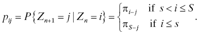
The inventory manager’s analyst uses knowledge about the distribution of demands and the Markov chain formulation to compute the stockout probability and the distribution of (or the expected value of) the number of FRUs that need to be ordered at the end of each month. An example of the kind of analysis needed to do this can be found in Chapter 3 of Ref. 22. See also Exercise 2.
This example is possibly the simplest inventory management scheme that has been studied quantitatively [17, 18, 22] . One clear disadvantage of this model is that it does not account for growth or shrinkage of the population of systems the inventory serves. Other variations may be needed to accommodate particular conditions in realistic inventory management applications. Fortunately, inventory management is one of the most widely studied operations research disciplines, and many models have been developed to enable quantitative inventory management under a dizzying variety of different operational conditions. Many of these models have been developed into open-source and commercial software. If you are considering using software for this task, the same review of its underlying model is needed as in any other sustainability engineering software to make sure that the assumptions the developers of the software made are close enough to your conditions that the results obtained from using the software will be relevant.
Again, systems engineers are not likely to be undertaking detailed work in support of a particular inventory management implementation, but they are more likely to be involved in determining requirements for the inventory management and in periodic reviews of data collection and analysis to verify continued satisfactory operation of the inventory. Seek help from operations research professionals, particularly if the operation you are studying has features that are not found in standard models.
13.2.1.2 A simple facility location model
Imagine that you are considering a repair scheme that incorporates an intermediate level of repair. The location of the intermediate repair facility or facilities has a great deal to do with the cost of the scheme. Ideally, one would like to locate the intermediate repair facility so that the sum of all relevant costs is as small as possible. Obviously, there is interplay between the facility location problem and the LoRA (Section 11.4.2) when the site of the intermediate repair facility is still to be determined. In this section, we will introduce a simple facility location model, again, not so much as a comprehensive model that you can use in many circumstances but more as an illustration of the relevant thought process.
Suppose that there are n systems in service, located at (x1, y1), . . ., (xn, yn) in the plane,3 that are to subtend one intermediate maintenance facility whose location (x, y) is currently undetermined. Its location will be determined by minimizing the total transportation costs from (x, y) to the n individual system locations, weighted by the amount of traffic expected to flow to and from each location. The transportation cost from (x, y) to (z, w) is given by a nonnegative real function C((x, y), (z, w)). The proportion of demands on the intermediate facility from system i is αi ≥ 0 with α1 + ⋅ ⋅ ⋅ + αn = 1. These may be unequal because there may be different numbers and types of systems at each site, and the demand for replacement FRUs is determined by the frequency of failures of each FRU type in each month and the total number of FRUs at the site. Then, the location of the intermediate facility may be determined by finding the (x, y) that minimizes
See Exercise 3. The cost function may also include a factor relating to delay. One of the reasons for carefully considering the location of an intermediate repair facility is to minimize logistics delay time (Section 12.4).
Again, this is possibly the simplest facility location model capturing the essential ideas. It is unlikely that it contains enough detail to be useful for realistic facility location problems, but sometimes a simple model is all that can be justified by the quality of the input information. In any case, it can provide some guidance even when all factors known to be important cannot be explicitly incorporated. There is an extensive research and pedagogical literature on facility location problems. Ref. 12 provides a way in.
13.2.2 Qualitative Supportability Assessment
Supportability assessment includes qualitative as well as quantitative techniques. Qualitative supportability assessment, which may also be used for developments in which the additional expense and time required to apply quantitative assessments via modeling may not be justified, or for which quantitative models don’t make sense, may be implemented in checklists for the adequate provision of
- comprehensive supportability requirements,
- diagnostic procedures,
- documentation,
- staff training, and
- test equipment,
and other related needs.
13.3 IMPLEMENTATION OF FACTORS PROMOTING SUPPORTABILITY
Several factors promoting supportability were listed in Section 12.2.2. Here we consider each of these in more detail and discuss their implementation and how they may lead to improved supportability.
13.3.1 Diagnostics and Fault Location
One of the most important factors in preparing for repair is the ability to determine speedily just what needs to be repaired. Obviously, repair can’t begin until the source of the failure is identified and located, and the longer it takes to do this, the greater the outage time and the worse it is for supportability and system availability. This section discusses some principles useful in designing systems so that faults can be speedily identified and located, paving the way for rapid initiation of repair.
When a failure occurs, time spent on diagnosing and locating the cause of the failure adds to outage duration. Supportability is improved by providing means for rapid diagnosis (what function failed and which part of the system is responsible) and fault location (identification of the specific subassembly or FRU that contains the fault). Online techniques for rapid diagnosis and fault location are procedures that run continually or periodically while the system is operating and include
- built-in test (BIT) facilities (also known as built-in self-test): BIT comprises means for ascertaining whether the system is producing proper outputs. Not only the final output but also intermediate outputs may be included. The diagnostic ability of BIT stems from an understanding of what a proper output should be for the stage under test, what the current output for that stage is, and how any differences indicate fault(s) that may have occurred in that stage. BIT may be implemented at the system level overall to help identify faulty FRUs and may also be implemented within an FRU to assist repair personnel if the FRU is repairable, either on-site or at a remote repair facility as dictated by the LoRA. See Ref. 30 for more information.
- parity checking and use of error-detecting (EDC) or error-correcting codes (ECC): these are a more rudimentary form of BIT because parity checking and EDC indicate only the presence of a fault but may not pinpoint the location of the fault. ECC provides additional robustness by correcting as well as detecting errors, but imposes a small penalty in throughput. The mathematical theory of error-correcting codes can be found in Ref. 25. Engineering applications are covered in Ref. 26.
- Diagnostic processes that run in background while the system is performing its functions.
Once the system has failed and is in an outage condition, off-line procedures may be applied. Off-line diagnostic and fault location procedures are tests and routines run using specialized test equipment and tools specifically designed to aid in determining the type and location of the fault(s) causing the failure. For example, a transmission test set for a specific digital communications mode (e.g., radioteletype) creates a signal of known integrity that is inserted into a transmitter input. The waveform is measured by the test set at predetermined test points in the transmitter and compared with the input. Deviations from known good signal quality at a certain test point indicate a difficulty with the transmitter stage(s) monitored by that test point. Physical design of the system can promote or impede supportability by making it easier or harder to access the required test points. Tests of this kind may also be automated if test points are brought out to a single external interface facilitating connection to a test set. These are not new ideas but are included here to provide examples of the design for supportability process.
13.3.2 Tools and Equipment
Some equipment is designed to be disassembled without tools. These systems, typically lower-value consumer products such as printers, implement snap fasteners that can be rapidly undone without any special tools (although specialized knowledge about the location and operation of the fasteners sometimes is required). But most more complex, higher-value systems intended to be used in more challenging environments usually require tools to undo fasteners, unseat circuit cards from connectors, etc. All such tools should be provided within easy reach so that time is not wasted searching for the proper tool.4 It is possible to write a contract calling for any special tools to be provided as part of the system’s physical design and to be shipped with the product. Some older examples include the R-390A/URR and Collins 51S-1 HF receivers, which were shipped with tools for disassembly and alignment incorporated into a compartment as an integral part of the receiver’s physical design. Ideally, the use of special tools should be minimized because ready availability of a common tool saves time should a tool be misplaced.
13.3.3 Documentation and Workflow Management
Maintenance staff may work with several different parts of a system if not different systems entirely. While training is necessary, the press of time sometimes means it is not sufficient, and staff may need to consult documentation to refresh their ability to execute required procedures. Time spent searching for and through documentation adds to outage duration. Each repair should be studied for proper workflow, and documentation should be integrated into the workflow so that it is readily available when needed. A disciplined process management approach [13, 28] should be followed so that inefficiencies are rooted out while opportunities for error are minimized.
Workflow management software provides step-by-step directions for carrying out particular repair tasks. It may also be useful for in-process quality control. Particularly complex or tedious procedures may benefit from support with workflow management software, increasing convenience and minimizing the chance for error. Workflow management software may also be of benefit to inexperienced maintenance staff by providing both real-time instruction and a supplement to training.
13.3.4 Staff Training
When repair personnel have not been trained in the procedures required for repairs carried out in their facility, excess time is consumed by various inefficiencies: looking up the proper execution of a step in the repair process, asking a colleague for help, figuring out the correct sequence of operations, etc. These add time to repair execution and decrease maintainability. The possibility of errors increases. Many studies show the positive return on investment from training [2, 6, 29] in a variety of areas. The value of training in repair operations, where actions are repetitive and errors have serious consequences, should not be underestimated.
13.3.5 Layout of Repair Facility and Workstation Design
While on-site servicing and repair is often performed under ad hoc circumstances, intermediate and higher-level repair is performed in dedicated facilities whose design and layout may promote or impede efficient execution of repair tasks. A permanent installation offers an opportunity to maximize efficiency and throughput by good design of the facility overall and of the individual workstations in the facility. A facility in which more time is consumed than necessary in repair suffers from reduced throughput, unwarranted delays in returning repaired items to useful service, and additional costs due to overstaffing.
The stochastic network flow model provides a fruitful approach to modeling layout of a repair facility. It requires understanding the mix of repair jobs to be performed in the facility as well as the individual steps needed for each repair job type. From the required steps, one can
- plan the layout of the facility and
- gather information about how long a job may spend at each workstation in the facility.
The latter is facilitated by maintenance task analysis (Section 11.3.2.2). Once these are known, a network flow model may be implemented. In this context, where the network usually has only one input node (a location in the facility where repair jobs enter the facility) and one output node (a location in the facility where repair jobs leave the facility), the network flow model resembles the precedence diagram method or critical path method. We present an example of a stochastic network flow model for a repair facility in the context of a performance (throughput and delay) analysis for the facility in Section 13.4.1.
Design of a maintenance facility should also include provisions for data collection and archiving to support a FRACAS as described in Chapter 5.
13.3.6 Design of Maintenance Procedures
While the layout of the repair facility and the flow of material through it greatly influence the time needed to complete a repair job, the procedures used for each step of the job are no less important. Facility layout covers the sequencing and placement of workstations. Design of maintenance procedures considers specification of the sequence of operations at each individual workstation. Design of maintenance procedures comprehends specification of
- test equipment needed to carry out the functions of the workstation,
- tools needed for disassembly, repair, alignment, reassembly, etc., to be accomplished at the workstation,
- a sequence of operations that will accomplish the tasks required at the workstation quickly while minimizing the chance for error,
- staffing of the workstation, including how many technicians are required and the duties of each,
- documentation to support the workstation’s operations, including overall process descriptions and detailed documentation for particularities of the system under repair,
- training for workstation operators, including periodic refresher training for experienced operators and introductory training for new operators,
- procedures for gathering management feedback from workstation operators to identify opportunities for greater efficiency, minimizing errors, and other factors that may become apparent only after experience is gained with existing operations, and
- continual improvement via periodic reassessment of workstation performance and redesign based on documented areas for improvement.
Workflow management software may also be useful in cases of a large number of inexperienced operators when there are few experienced operators they can learn from, and in cases where traceability of operations or material is required.
13.3.7 Spare Parts, Repair Parts, and Consumables Inventory
In any repair scheme, multilevel or not, in which repairs are performed by replacing modules or subassemblies (referred to as line-replaceable units or FRUs), a stock of known-good units is needed that is readily accessible to repair staff. Usually, this means some number of spare units will be kept at each site where repair using those units will be performed. How is that number chosen?
Support management tries to balance the costs of acquiring and carrying an inventory of spare units against the costs incurred when a repair requiring a certain type of unit cannot be completed in a timely fashion because the inventory of that type of unit on the site is depleted. Most early inventory optimization models involved finding an optimal value for the stockout probability (Section 12.4). When the stockout probability is low, a larger number of spare units are required, and acquisition and carrying costs are high. When the stockout probability is high, uncompleted repairs will occur more frequently, and the costs due to emergency acquisition of spare units and to longer outages increase. The sum of these costs should have a U-shaped graph, and from this formalism, an optimal value of the stockout probability, depending on the particular values of the costs involved, may be selected. Again, this is likely the simplest inventory optimization model that has been studied quantitatively, and it is not likely to apply directly in many particular cases. Many realistic inventory optimization models have been considered in an extensive operations research literature. See also Ref. 11 for an overview.
Failures and outages are not divorced from availability, however, and most systems have some availability objective. So, for instance, if an outage persists for a longer time because a spare unit is not present in the on-site inventory, then the system availability (any of inherent, operational, or achieved, see Section 10.6.4) will decrease. In a sense, stockout probability is a proxy for system availability: the reason one wants to keep the stockout probability low is so that the system availability will be high. The presence of an availability requirement means that this may be addressed directly by making the system availability requirement a constraint in formulating the inventory sizing optimization. In this way, system supportability is arranged so that the system availability requirement is directly considered—a more holistic approach integrating supportability and reliability. Some examples of this approach include Refs. 1, 7, 23.
A great variety of models have been developed to cover the many different operational possibilities in use: spares kept on-site only, spares kept on-site with backups kept at an intermediate serving location that provides backup spares for several sites, spares ordered directly from the manufacturer, etc. Many of these can be found in Ref. 27.
In practice, most enterprise management software contains inventory optimization and management features, and it would be rare to need to develop a new model from scratch. As with all contemplated software applications, it is worthwhile to check the assumptions used by the software’s provider to make sure that they are compatible with the operation and results needed. Tuning after implementation may be desirable if experience indicates that the numbers suggested by the software are too large or too small.
13.3.8 Transportation and Logistics
A multilevel repair scheme requires extensive transportation of items to be repaired, repaired items, spare parts, etc. The more levels and locations in the scheme, the more transportation required. Transportation and logistics typically is the largest component of cost in these schemes, after acquisition costs and labor costs. Optimal facility location (Section 13.2.1.2) is one way to minimize transportation costs. However, it is often the case that facilities cannot be located at will, for example, in cases where one may wish to exploit legacy infrastructure already in place. In such cases, it is still important to try to minimize transportation costs and delays. When locations (system installations, intermediate and higher-level repair locations) are fixed, some of the factors that influence transportation and logistics costs include
- the mix of transportation modalities used for different routes in the repair scheme,
- batching and staging of jobs and material for transport, and
- internal versus subcontracted transportation.
Formal optimization models may be devised for cost minimization considering these factors. In many cases, simpler accounting models similar to the LoRA may be adequate to provide a good starting point for the operation, which may then be tuned after some experience is gained with its operational properties.
13.4 QUANTITATIVE DESIGN FOR SUPPORTABILITY TECHNIQUES
Most supportability engineering concerns actions taken by support staff working in a system whose goal is the promotion of speedier, less costly, and less error-prone repair. Section 13.3 discussed some important factors whose proper implementation helps promote better supportability. Some of these factors may be dealt with quantitatively, and so they may be settled by optimization. Earlier in this chapter, we considered some elementary quantitative developments for inventory management and facility location, showing the most basic models that apply and pointing to the literature for further developments. In this section, we will consider some more detailed models for the layout of a maintenance facility and staff sizing for individual workstations so that these may be designed to achieve stated supportability requirements at minimum cost through optimization of the control parameters available.
13.4.1 Performance Analysis of a Maintenance Facility
Some maintenance facilities are designed to support many system types, and many different types of repairs may be performed there. For instance, in the multilevel model studies in Section 11.4, more complicated repair demands are aggregated from field deployment sites and are serviced according to some planned scheme. Supportability concerns itself with enabling speedier repairs, so it is of interest to know how the design of the maintenance facility may promote or inhibit speedy repairs. This Section discusses a simple model that can be used to study the performance of a maintenance facility. Commonly used performance effectiveness criteria include throughput (the number of units flowing from the entrance of the facility to the exit of the facility per hour) and delay (the amount of time a unit spends in the facility waiting and undergoing service). The model may be used as a basis for optimization of the facility by adjusting the quantities and arrangement of workstations so that throughput and delay requirements are met at lowest cost.
Maintenance facilities commonly consist of some number of workstations that may be all the same (if there is only one type of repair being performed there) or different (if the facility handles more than one type of repair). Units undergoing maintenance enter the facility and routed to an incoming inspection and sorting activity, from where they are sent to the proper workstation. They then may be routed to other workstations if additional maintenance is needed and are routed to an exit when all maintenance is complete. It is common to refer to units requiring maintenance as “jobs.” So one can picture a maintenance facility as a collection of workstations and streams of jobs flowing around the workstations. A convenient quantitative model for this activity is a flow network [14] in which an exogenous demand of jobs enters the network, spend some time at various workstations in the network, and leave the network when their required maintenance is complete.
In addition, in most cases,
- the number of persons staffing each workstation is limited, and
- the amount of time a job spends at a workstation is not predictable in advance.
So the network is actually a network of queues [3, 8, 19], where by a “queue,” we mean a service system subject to random demands, and the time required to service each demand is random too. Each workstation is represented as a queue in which the number of servers is the number of operators attending that workstation, and the service times are the (random) times it takes to complete maintenance at that workstation (see maintenance task analysis, Section 11.3.2.2). The flow of jobs in the network is described by a Markov process having a transition matrix whose (i, j) entry is the conditional probability that a job will travel next to workstation j given that it is now at workstation i. This routing model also accommodates fixed, deterministic routing in which the path of a given job type through the facility is fixed and determined in advance. Routing is determined by the sequence of maintenance operations required by a unit, the capabilities of each workstation, and, in case there is more than one workstation having a given capability, the random completion times of jobs at workstations. Figure 13.1 shows a typical model of this sort of operation.
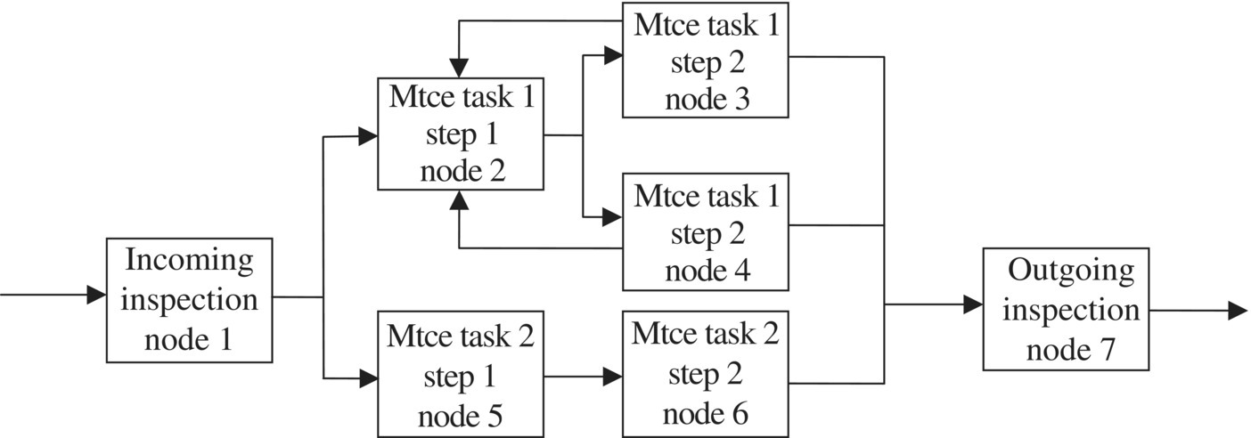
Figure 13.1 A maintenance facility flow network.
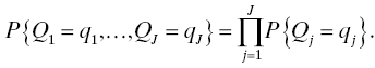
In this example, there are two different maintenance tasks because there are two types of units being serviced at this facility. Each task has two steps. The second step of Task 1 is more time consuming than the others, so two workstations are provided for this step.5 The path from Task 1 step 2 back to Task 1 step 1 represents possible rework due to erroneous execution of Task 1. Jobs arrive from outside the network (call this node 0) and exit to outside the network when they are completed. Each workstation may be thought of as a queue with an arrival process composed of the jobs waiting to be worked on at the workstation, the number of servers equal to the number of people staffing the workstation, and the service times equal to the time required to complete a job at that workstation. A routing matrix for this example network is (rij : i, j = 0, 1, . . ., 7) (Figure 13.2).
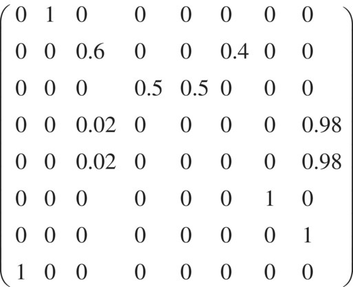
Figure 13.2 Example routing matrix.
This matrix represents that approximately 60% of the jobs entering the facility are of type 1 and 40% are of type 2. Half the completed jobs from step 1 of Task 1 (node 2) are sent to the workstation at node 3, and the other half are sent to node 4. The diagram and matrix represent that 2% of the jobs leaving nodes 3 and 4 need to return to node 2 because Task 1 was not completed correctly. All jobs receive an outgoing inspection before leaving the facility. This network is considered open because there is at least one node where jobs may enter or leave the network (in a closed network, a fixed number of jobs circulate around the network, no new jobs may enter, and no jobs leave the network; a closed network is usually not appropriate for modeling a repair facility because jobs are intended to be completed and leave the facility).
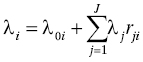
The simplest queuing network model is the Jackson network [19, 20] in which each individual workstation is an M/M/c FCFS6 queue [15], and the routing is Markovian (where a job goes next depends only on where it is now, and not on any of its prior location(s)). The Jackson network allows for only one job class,7 but Poisson traffic may arrive from outside the network at any node, jobs may leave the network at any node, and load-dependent arrival and service rates are supported. The key feature of the Jackson network is that it has what is called a product-form solution. That is, the joint distribution of the number of jobs at each workstation may be written as the product of the individual distributions of the number of jobs at each workstation. In other words, the network behaves as though the individual workstations were stochastically independent. This result depends crucially on Burke’s theorem [5], which asserts that the departure process from an M/M/c queue is also a Poisson process. Formally, let J denote the number of workstations in the Jackson network, let Ni denote the number of jobs in service at workstation i in equilibrium,8 and Qi denote the (equilibrium) total number of jobs at workstation i (i = 1, . . ., J) (i.e., in service and waiting). Then the product-form solution asserts that
and
Denote the service rate for a single server at workstation i by μi and the number of servers at workstation i by ci (i = 1, . . ., J). Then, the total service rate at workstation i is ciμi. The number of servers ci at workstation i is a control variable in optimizing the facility.9 The number of operators to be assigned to each workstation changes the service time for jobs at that workstation and also affects waiting times and buffer occupancies. Typically in maintenance operations, each workstation has only a finite buffer space, or “waiting room,” and the buffer size may be a control variable in optimization, but the Jackson network model allows only infinite buffers. While this is clearly only an approximation to the real maintenance facility design, in applications, one would choose a buffer size large enough to accommodate most anticipated demand because one would not allow materials waiting for service to be ignored, discarded, or otherwise leave the system without receiving attention.
The first step in solving a Jackson network problem is to determine the composite arrival rates at each node when both the exogenous arrivals and the arrivals routed from other network nodes are included. This is done by solving the traffic equation
where λi is the composite arrival rate at node i, λ0i is the exogenous arrival rate at node i, and rij is the (i, j) entry in the routing matrix R (rij = P{job next visits workstation j | job is currently at workstation i}). Let λ and λ0 be row vectors containing the individual λi and λ0i values. Writing the traffic equation in matrix form as λ(I − RT) = λ0, we readily obtain the composite arrival rates λ = λ0(I − RT)−1. I − RT is invertible because the network is open [8] . Knowing each composite arrival rate allows the individual workstations to be analyzed as M/M/ci queues. We write ρi = λi/ciμi, i = 1, . . ., J. A sufficient condition for the existence of an equilibrium solution for the M/M/ci queue is ρi < 1. The probability that there are no jobs (either waiting or in service) at workstation i is

Some performance variables of interest at workstation i are [15]
- The expected number of jobs in the buffer at the workstation is

You will want to be sure there are enough buffer spaces to accommodate at least this many queued jobs plus maybe some margin for those times when the buffer occupancy exceeds its mean.
- The expected total number of jobs at workstation i, including both waiting and in service, is
- Wi is the time a job spends waiting for service (in the buffer) at workstation i. Its expected value is
- Let Ti denote the total time a job spends at workstation i, including waiting time and service time. Then, with Si denoting the service time for a job at workstation i,

- Assuming that the maintenance facility has one node at which jobs enter (call it node a) and one node at which jobs leave (call it node b) (these are nodes 1 and 7, respectively, in the earlier example), the expected time it takes for a job to complete a trip through the maintenance facility is the (a, b) entry in the matrix

where I is the identity matrix, R is the routing matrix for the facility, S is a matrix whose (i, j) entry is Ti + τij (τij is the expected transit time from node i to node j; in most cases, this will be taken to be zero unless the transit time is not negligible compared to the average service and wait times), and (S#R)ij = Sij⋅Rij (this is called the Hadamard or direct product of S and R) [31].
- The throughput is the expected number of jobs leaving the exit node b per unit time. Node b is an M/M/cb FIFO queue with composite arrival rate λb (from the traffic equation) and service rate μb. By Burke’s theorem, the departure rate from node b is also λb, and this is the throughput expressed in the time unit of the composite arrival rate.
The performance parameters of the queueing network model used for the maintenance facility can be used as variables in a scheme to optimize the performance of the facility. The objective for this optimization could be to minimize the total time a job spends in the facility, maximize the throughput, minimize the total cost of the operation, etc., as required by the economics of the system. Full exploration of maintenance facility optimization is beyond the scope of this book, but you can use the simple Jackson network analysis summarized earlier to get some guidance on an initial design. More elaborate or more detailed queueing network models are available and would be appropriate to use if the quality of your information about the input parameters (arrival processes, service time distributions, etc.) warrants this sharper pencil. Given the uncertainty in many systems like these in which human performance is a major factor, the Jackson network model is often all that can be justified. Related models have been considered in the literature, including Refs. 10, 16.
The model discussed in this section makes strong assumptions about the operation (Poisson arrivals, exponential service, etc.), which may or may not be valid in particular cases. As always, the need to use a sharper model (one that better matches known characteristics of the true maintenance situation) is guided by the economics of the system development. In most cases, the simple model can provide useful guidance for facility design and optimization, and you are better off using it rather than nothing. Spend additional resources in fine-tuning a more complicated model only if the economics justifies the additional cost.
13.4.2 Staff Sizing: The Machine Servicing Model
A key to planning for efficient maintenance is the choice of an appropriate number of personnel to carry out each maintenance task. In this section, we introduce a quantitative approach to staff sizing by adapting a standard industrial engineering queueing model, the machine servicing model, to this need. The number of technicians at workstation i is ci in the notation of Section 13.4.1, so there is an interplay between this workstation staffing model and the performance analysis considered earlier. When optimizing a facility using the earlier performance analysis model, the model in this section provides a good starting point for ci. The cumulative effect of these choices becomes visible when the whole network model is executed.
The machine servicing model is a finite-source queueing model. That is, there are only a finite number of sources generating jobs for the queue. These sources are the machines requiring service from time to time (when they break down). The servers are the repair personnel. In this adaptation, we take the number of sources, S, to be the number of products, systems, or services generating maintenance tasks to be performed at a given workstation and c, the number of servers, to be the number of technicians who carry out the tasks at that workstation. In the planning exercise, c is unknown and is to be chosen to minimize some operational effectiveness measure such as the total time required to carry out all required maintenance operations or the total cost of the maintenance operation at the workstation. The rate at which the sources demand service from the maintenance staff is related to the frequency of failures of the products, systems, or services covered by the maintenance facility and the number of products, systems, or services served by the maintenance facility. The service times in the queueing model are the outage durations. Our initial model treats these as given (having a known distribution) and uses c as a control variable. A more-advanced model can be constructed using also the distribution of the service times (the outage times) as a control parameter. In that case, there is an interplay between the number of servers and the service times that makes the model analytically more complicated, but simulation can be used to obtain results from this more realistic model.
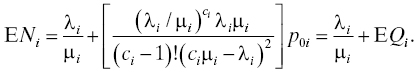
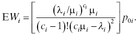
In this section, we will consider a simple machine-servicing model that makes several simplifying assumptions so that you can get an idea of what this technology can do without getting bogged down in details. More realistic models can be developed, often requiring simulation for solution, when there is a need for greater precision. Accordingly, we assume that there are S products, systems, or services of the same type assigned to the workstation in question, and each is a repairable system whose failures appear in time as homogeneous Poisson processes [22] with rate λ. The arrival rate of jobs to the c-server queue that is the maintenance staff is λn = (S – n)λ when n, the number of systems currently in service is < S, and λn = 0 when n ≥ S. We postulate that the repair time for one system is exponentially distributed with mean 1/μ, so overall the repair times for all the systems in the facility are exponentially distributed with mean 1/μn = 1/nμ for 0 ≤ n < c and 1/μn = 1/cμ for n ≥ c. Write ρ = λ/μ and assume that ρ < 1. Solution of this model uses the theory of birth-and-death processes [22], from which we may obtain useful equilibrium operating characteristics of the model [15] :
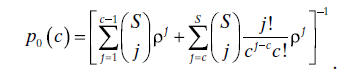
- The probability that there are i systems being serviced is

where p0 is the probability that the facility is idle, given by
- The expected number of systems at the workstation, including those being serviced and those waiting, is given by

- The expected number of systems waiting for service is given by

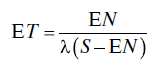
- The expected time that a system spends at the workstation is given by
and the expected time that a system spends in the buffer waiting for service is given by

When using this model to plan the number of operators to staff a workstation, choose a supportability figure of merit (such as the expected number of systems waiting for service) and use c as a control variable in the appropriate expression (we have written the idle probability as p0(c) to emphasize this), minimizing it with respect to c within a given cost constraint.
Again, even though this may look complicated, it is possibly the simplest machine-servicing model that has been treated quantitatively, and it may not contain all the details of a particular operation. In practical cases, though, it provides better guidance than guesswork for a starting point, and it doesn’t take long before any inadequacies in the operation become apparent so that adjustments may be made from a sound baseline.
13.5 CURRENT BEST PRACTICES IN DESIGN FOR SUPPORTABILITY
13.5.1 Customer Needs and Supportability Requirements
Supportability has a direct impact on outage durations, so it is important to understand the customer’s needs for the speed of service restoration so that they can be folded into supportability requirements. For example, the customer may have a need for a failover time (Section 11.3.1) not exceeding 50 milliseconds. This can only be achieved with automated processes, so all support aspects of bringing a redundant unit online need to be worked out in advance. These aspects include diagnosis and fault location, test of the redundant unit (if necessary), and predetermination of what is to happen if the switchover to the redundant unit does not complete properly. Supportability requirements should address at least the aspects that bear directly on decreasing the length of outages. These include
- diagnosis and fault location time,
- on-site spares inventory management,
- dispatch time for technicians to reach the faulty replaceable unit, and
- procedures for error minimization during replacement.
13.5.2 Team Integration
As with maintainability engineering, a significant danger to be avoided with supportability engineering is beginning to consider supportability too late in the development process. For example, we have seen how an important supportability consideration, namely, the proper sizing of spares inventories, has an effect on system availability. Given an availability requirement, and many systems have these, it pays to begin an inventory optimization early in development so that information is available for downstream use, for example, in the LoRA.
It is not reasonable to expect every team member to be an expert in supportability, so “omnibus” development management meetings, in which representatives from all sustainability engineering areas are involved, help ensure that important supportability issues do not escape attention. When a team member hears a plan from another part of the team that has an impact on supportability, immediate coordination can take place, and better results obtained.
13.5.3 Modeling and Optimization
When there is an opportunity to use new facilities or processes in maintenance, these should be planned on the basis of some quantitative modeling, even if only simple modeling. This chapter has shown examples of modeling applied to inventory management, facility location, maintenance facility design, and maintenance workstation staffing. The models shown here cannot support every plan in these four areas, but they are intended to show the reasoning process used when using quantitative methods for these plans. Most enterprise management software contains integrated models for these kinds of plans, but not every organization uses enterprise management software, and even for those that do it pays to verify that the assumptions on which the software is predicated reasonably match the conditions of your applications. Models don’t need to be (indeed, can never be) perfect, but they do provide guidance that is better than guesswork for initial design of supportability facilities and processes.
13.5.4 Continual Improvement
It is rare that the initial design for supportability produces stellar results. Tuning of the control parameters in any facility or process is almost always needed. But beyond that, continual improvement is always of value even when support processes are functioning well. Conditions change: failures occur more or less frequently, suppliers come and go, staff turnover increases or decreases, etc., so what worked well a few months ago may no longer be optimal. A healthy program of continual improvement helps keep support costs lower while keeping results where they need to be. Continual improvement is supported by adapting quality control and management tools to support process needs. For instance, facility throughput may be monitored with a control chart so that when throughput changes, it is possible to determine whether the change is due to some important factor in the facility’s operation (a “special cause”) or whether it is a reflection of the normal statistical fluctuation present in any process that is subject to random influences or “noise variables” (a “common cause”).
13.6 CHAPTER SUMMARY
This chapter has been devoted to actions you can take to improve the supportability of a design. Design for supportability is similar to design for reliability and design for maintainability in that it attempts to anticipate the support environment a system or service will live in and optimize operational conditions to deliver a level of support consistent with customer needs and the system’s or service’s business case. Instead of trying to prevent failures or optimize maintenance, design for supportability develops actions that can be taken to improve the support environment so that the overall goal of speedy, low-cost, and error-free repair can be achieved. Some of the specific aspects of a system’s support environment that are covered here include inventory management for spare parts and consumables, location of intermediate repair facilities, arrangement of a repair facility to optimize throughput and cost, and choosing a good staff size (number of operators) for a repair workstation. Other characteristics of the support environment that design for supportability covers include procedures and tools for failure diagnostics, fault location, logistics management, documentation and training, and design of maintenance procedures. The chapter is designed to help systems engineers become familiar with basic supportability principles and only in a few cases pursues development of models in detail. Textbooks for the details of supportability engineering include Refs. 21, 24.
13.7 EXERCISES
- Suppose X1, X2, . . . are random variables having an exponential distribution with mean μ1 and that Y1, Y2, . . . are random variables having an exponential distribution with mean μ2. Show that the combined population X1, Y1, X2, Y2, . . . has an exponential distribution with mean (μ1−1 + μ2−1)−1. Does this work for more than two populations?
- Determine the stockout probability for the (6, 9) inventory management system when the demand distribution is Poisson with rate 4.
- Consider the facility location model described in Section 13.2.1.2. Find the location of the intermediate facility when there are four systems located at (0, 0), (10, 0), (1, 11), and (17, 24); each system sends the same demand on the intermediate facility; and the cost function is
 .
.
REFERENCES
- 1. Adams CM. Inventory optimization techniques, system vs. item level inventory analysis. 2004 Annual Reliability and Maintainability Symposium . January 26–29; Piscataway, NJ: IEEE; 2004. p 55-60.
- 2. Bartel AP. Measuring the employer’s return on investments in training: evidence from the literature. Ind Relat J Econ Soc 2000;39 (3):502–524.
- 3. Baskett F, Chandy KM, Muntz RR, Palacios F. Open, closed, and mixed networks of queues with different classes of customers. J ACM 1975;22:248–260.
- 4. Bolch G, Grenier S, de Meer H, Trivedi K. Queueing Networks and Markov Chains: Modeling and Performance Evaluation with Computer Science Applications. New York: John Wiley & Sons, Inc; 1998.
- 5. Burke PJ. The output of a queueing system. Oper Res 1956;4 (6):699–704.
- 6. Carnevale AP, Schulz ER. Return on investment: accounting for training. Train Dev J 1990;44 (7):S1–S32.
- 7. Chan CK, Tortorella M. Spares inventory sizing for end-to-end service availability. Proceedings of the Annual Reliability and Maintainability Symposium; January 22–25; Philadelphia, PA; 2001. p 98–102.
- 8. Chen H, Yao DD. Fundamentals of Queueing Networks. New York: Springer; 2001.
- 9. Conway AE, Georganas ND. Queueing Networks—Exact Computational Algorithms. Cambridge: MIT Press; 1989.
- 10. Crespo Marquez A, Sánchez Heguedas A. Models for maintenance optimization: a study for repairable systems and finite time periods. Reliab Eng Syst Saf 2002;75 (3):367–377.
- 11. Davis RA. Demand-Driven Inventory Optimization and Replenishment: Creating a More Efficient Supply Chain. Hoboken: John Wiley & Sons, Inc.; 2013.
- 12. Drezner Z, editor. Facility Location: A Survey of Applications and Methods. New York: Springer-Verlag; 1995.
- 13. Dumas M, LaRosa M, Mending J. Fundamentals of Business Process Management. New York: Springer-Verlag; 2013.
- 14. Ford LR, Fulkerson DR. Flows in Networks. Princeton: Princeton University Press; 1962.
- 15. Gross D, Harris CM. Fundamentals of Queueing Theory. New York: John Wiley & Sons; 1974.
- 16. Hani Y, Amodeo L, Yalaoui F, Chen H. Simulation based optimization of a train maintenance facility. J Intell Manuf 2008;19 (3):293–300.
- 17. Heyman DP, Sobel M. Stochastic Models in Operations Research. Mineola: Dover Publications; 2003.
- 18. Hillier FS, Lieberman GJ. Introduction to Operations Research. 8th ed. New York: McGraw-Hill; 2005.
- 19. Jackson JR. Networks of waiting lines. Oper Res 1957;5:518–521.
- 20. Jackson JR. Jobshop-like queueing systems. Manag Sci 1963;10:131–142.
- 21. Jones JV. Supportability Engineering Handbook: Implementation, Measurement and Management. New York: McGraw-Hill; 2006.
- 22. Karlin S, Taylor HM. A First Course in Stochastic Processes. 2nd ed. New York: Academic Press; 1975.
- 23. Kumar UD, Knezevic J. Availability based spare optimization using renewal process. Reliab Eng Syst Saf 1998;59 (2):217–223.
- 24. Kumar UD, Crocker J, Knezevich J. Reliability, Maintenance and Logistic Support: A Life Cycle Approach. Dordrecht: Kluwer Academic Publishers; 2000.
- 25. MacWilliams FJ, Sloane NJA. The Theory of Error-Correcting Codes. Amsterdam: North-Holland; 1977.
- 26. Michelson AM, Levesque AH. Error Control Techniques for Digital Communications. New York: John Wiley & Sons, Inc; 1985.
- 27. Muckstadt JA. Analysis and Algorithms for Service Parts Supply Chains. New York: Springer; 2005.
- 28. Sharp A, McDermott P. Workflow Modeling: Tools for Process Improvement and Application Development. 2nd ed. Norwood: Artech House; 2008.
- 29. Stolovitch HD, Maurice JG. Calculating the return on investment in training: a critical analysis and a case study. Perform Improv 1998;37 (8):9–20.
- 30. Stroud CE. A Designer’s Guide to Built-In Self-Test. New York: Springer-Verlag; 2002.
- 31. Tortorella M. Path-additive functionals in stochastic flow networks with Markovian routing. Rutgers University Department of Industrial and Systems Engineering Working Paper #06-004; 2006.