
6
Design for Reliability
6.1 WHAT TO EXPECT FROM THIS CHAPTER
Now that we have a good grasp of reliability requirements and some quantitative modeling supporting them, we turn to the question of how to arrange a design so that reliability requirements can be met. The development team needs to take deliberate actions to build reliability into the product or service. Without this attention, the product or service will have some reliability, but it will be just whatever you get by chance. You need to take control of system reliability and take positive steps to drive it in the direction you want, as summarized in the reliability requirements. This chapter discusses several techniques that you can use to build reliability into the product or service, an activity we call “design for reliability.” These include:
- a thorough understanding of the reasoning process underpinning design for reliability,
- a CAD tool for design for reliability in printed wiring boards (PWBs),
- fault tree analysis (FTA),
- failure modes, effects, (and criticality) analysis,
- a brief introduction to design for reliability in software, covered in more detail in Chapter 9, and
- robust design as a reliability enhancement tool.
As with many of the ideas in this book, none of these receives an exhaustive treatment because they are each treated thoroughly elsewhere (references provided) as individual technologies in their own right. The primary intent here is to show how these apply in reliability engineering specifically and to give you the right material so that
- you can use these in your systems engineering practice and
- you are prepared to dig into any of these more deeply should you have need or interest.
6.2 INTRODUCTION
Our focus up to this point has been on writing appropriate and effective reliability requirements. When this task is completed, systems engineers still have a stake in the success of the project, and can add value by promoting efficient achievement of these (and other) requirements. In reliability engineering, the most effective tool available to do this is design for reliability. Design for reliability is the set of activities undertaken during product or service design and development to realize the product or service so that it meets its reliability requirements. In brief, design for reliability encompasses those actions taken during product or service design and development to anticipate and manage failures. “Manage failures” means to
- avoid those failures for which economically sensible countermeasures can be devised, and
- plan for how to react to failures when they do occur.
Design for reliability is a systematic, repeatable, and controllable process whose goal is to fulfill reliability requirements in an economically sensible way. This chapter covers not only the basics of design for reliability but also some deeper aspects of this process when applied in the specific domain of PWBs in electronic systems. Parts II and III of this book discuss maintainability and supportability procedures to minimize the duration of outages that take place when failures occur.
Design for reliability is most effective when it takes place early in product or service development. Because the product or service is not yet realized, a way is needed to assess the likelihood that its reliability requirements will be met so that product/service design actions to achieve reliability requirements can be guided. Accordingly, the first topic covered in this chapter is reliability assessment of a notional product or service, that is, one that is not yet real but whose development is starting or is partially completed. Reliability assessment is a way to tell where you are and provide feedback to the development team.
Design for reliability will not eliminate all possible failures. Design for reliability is a special kind of attempt to predict the future, and, as such, has the usual potential for errors of omission and commission. There are many examples of comprehensively executed failure mode and effects analyses (FMEAs) that described many potential failure modes in detail but completely missed a failure mode that caused many failures in service. One example is the Saturn seat recliner failure described in a 2000 National Highway Transportation Safety Administration case [22]. Because such omissions can easily occur, it is important to maintain a robust program of learning from past experiences. We return to this point in the design for reliability process description.
Design for reliability leads naturally into design for maintainability and design for supportability because it is important to provide the customer with means for dealing with failures that may occur. While design for reliability does provide a robust approach to failure prevention, it is misguided to imagine that all failures can be prevented. Failures will occur. The key question is how will the supplier also create the means for customers and users to minimize the impact on their operations of the failures that do occur. This is the content of design for maintainability and design for supportability that you will find in Chapters 11 and 13.
6.3 TECHNIQUES FOR RELIABILITY ASSESSMENT
There are important reasons for being able to assess product or service reliability throughout the life cycle. During design and development, we need a basis for design for reliability activities: it will be difficult to tell whether further improvement may be needed unless a reading of current status of reliability is available. During product manufacturing or service deployment, it is important to assure that related processes are not introducing into the product or service latent defects that may activate and cause failure later on. During operation and use by the customer, all parties are concerned with whether the product or service is meeting its reliability requirements. This section discusses quantitative reliability modeling and reliability testing as a means for assessing reliability during design, development, and manufacturing for products. Design for reliability for services is covered in Chapter 8. The all-important question of estimating reliability from data gathered during the customer’s use of the product was covered in Chapter 5.
6.3.1 Quantitative Reliability Modeling
All of Chapters 3 and 4 were devoted to an exploration of quantitative reliability modeling for systems engineers. Quantitative reliability modeling is usually the domain of reliability engineering specialists, and these chapters go more deeply into this subject than is usually required of systems engineers. The material presented in Chapters 3 and 4 is to
- help guide systems engineers so that they can be good suppliers to, and customers of, reliability engineering specialists, development management, and other stakeholders,
- provide a solid foundation for further exploration of reliability modeling if that is needed or desired, and
- promote correct use of language and concepts that is so important for clarity of purpose and communications.
It is fruitful to incorporate a good customer–supplier model into the systems engineering process for dealing with sustainability specialists. While this is rarely done explicitly, all parties can benefit from understanding that there is a customer–supplier interaction talking place here and even an informal acknowledgment of that relationship can lead to more effective behavior and results. As detailed in Chapter 1, the system engineer supplies reliability requirements to the development team and is a customer for the reliability assessments and data analyses supplied by the reliability engineering staff. Common understanding and correct use of language is a necessary condition for this to be successful. Development management are also suppliers and customers for systems engineering. They provide development schedules and financial goals, insight into customer needs, and funding for project work. In turn, they need up-to-date and unvarnished information about current status of important project attributes, including reliability, maintainability, and supportability. Other stakeholders include customer representatives, with whom various negotiations go on concerning needs and likely outcomes in sustainability parameters, and executives on both sides of the table. Systems engineers are adept at managing all these interfaces, and the more knowledgeable they can be concerning these important factors, the more likely the system or service will be successful: desirable to the customer and profitable to the supplier.
We can use quantitative reliability modeling when a product is in the conceptual stage. No hardware or software or even prototypes need yet exist; modeling is the construction of a mathematical representation of the system and its constituent components that allows estimates or predictions about reliability of the components to be combined in a systematic way to yield estimates of the reliability of the system and its subsystems. Such modeling serves as one of the indicators that systems engineers can use to help decide whether resources need to be added (or may be taken away) to keep the anticipated reliability of the system at the level specified by the system reliability requirements. Information gained from reliability modeling should always be used by design teams to determine where designs may need to be strengthened when the modeling shows that there is significant chance that requirements will not be met.
Reliability modeling without use of the results by design teams is a wasted effort.
6.3.2 Reliability Testing
While testing as a means for reliability assessment can sometimes be helpful, there is usually little opportunity at the early stages of development for learning about the reliability of the system by testing. This is not to say that there are not valuable things that may be learned about a system by testing prototypes or early versions, or components and subassemblies that may be assembled into the system, but reliability testing specifically requires testing of a large number of units for a long time (typically, several multiples of the anticipated mean lifetime of the unit), and this is not practical during early development. This is one of the primary reasons why we urge systems engineers to employ reliability engineering and design for reliability techniques early in the system development process. The details of designing and interpreting reliability tests, including accelerated life tests, are beyond the scope of this book. Many excellent treatments are available, including Refs. 2, 14, 25, 29, 35, and others.
There is one notable exception to this principle. In contemporary practice, testing is the primary (though not the only) tool used for learning about reliability in software products or systems. Thorough discussion of this approach is contained in Chapter 9. What makes reliability testing viable for software products or systems is that the effects of software failure mechanisms are immediate. The standard model for software failures is that most root causes are faults in the code, and when a requirements-legal input condition1 tendered to the software invokes that part of the code where a fault resides, an improper output results. “Improper” means “different from what it should be according to the requirements” so the improper output is a failure. This happens with essentially no delay whenever such an input condition is tendered, and it happens in the same way in every copy of the software (barring reproduction errors that are usually assumed to be rare or nonexistent). Reliability testing for software is practical because
- unlike in hardware, failure occurs instantly when a failure mechanism is activated,
- failure mechanisms are stimulated by specific input conditions, so testing may proceed by searching the space of possible input conditions, and
- faults may be corrected more quickly than they could be in hardware.
This kind of testing is facilitated by use of an operational profile which is a catalog of requirements-legal input conditions together with estimates of the probability that each will be encountered in service. More details are given in Chapter 9. See also Refs. 13, 36.
6.4 THE DESIGN FOR RELIABILITY PROCESS
The purpose of this section is to explain the abstract or generic thought process used in design for reliability. This process uses reasoning similar to FTA, and it can be convenient to use a tree-like diagram for summary of results and communication. See Ref. 8 for further comprehensive review of this topic.
The design for reliability (DFR) process that we describe here is a systematization of the idea that DFR proceeds by anticipation and management of failures. Each design choice has reliability consequences. In other words, each design choice introduces some potential failure mode(s) into the product or service. The DFR process catalogs those failure modes, determines the failure mechanisms and root causes associated with each failure mode, considers what preventive action(s) may be taken to prevent those failure mechanisms from becoming active, and lists the consequences of taking, or choosing not to take, the preventive action(s). This process may be visualized in the form of a tree (see Figure 6.1).
Figure 6.1 Design for reliability process tree.
The diagram is necessarily incomplete because lack of space prevents explicit representation of all the failure modes, failure mechanisms, preventive actions, and consequences that stem from even the single design choice shown in the diagram. In practical cases, moreover, the number of developed failure modes from any given design choice is likely to be small, and a formal study of this nature, which may turn out to be costly if fully pursued, is likely to be reserved for truly critical design choices.
To use the DFR process, proceed from left to right in the figure. The first step is to determine the failure modes introduced into the system by each design choice. This can be done systematically by reviewing each system requirement and listing the ways that the design choice can contribute to violation of the requirement. For example, the designer of a low-voltage power supply can choose aluminum electrolytic or tantalum electrolytic capacitors for filtering. For aluminum electrolytic capacitors, relevant failure modes include open-circuit failure, short-circuit failure, capacitance change, leakage current increase, open vent, and electrolyte leakage [23]. For these capacitors, k = 6 in Figure 6.1. For tantalum electrolytic capacitors, relevant failure modes include short-circuit failure and thermal runaway failure, and in Figure 6.1, k = 2 [26]. The design choice, which includes the voltage to be applied to the tantalum capacitor, may stimulate or suppress relevant failure modes in the capacitor, depending (in this case) on the voltage applied by the circuit.
The next step in the process is to associate with each failure mode listed in the first step the relevant failure mechanisms. There is often more than one failure mechanism for each failure mode. Failure mechanisms should be developed in enough detail so that root causes may be identified. That is, each statement about a failure mechanism should include the results of root cause analysis so that appropriate countermeasures may be discerned. For aluminum electrolytic capacitors, section 4 of Ref. 23 shows the failure mechanisms associated with each of the six failure modes listed earlier. For example, the short failure mode is caused by isolation failure in the dielectric film or a short between the electrodes. In turn, isolation failure in the dielectric film is due to localized defect(s) in the oxide film or dielectric paper weakness. This analysis continues until enough is understood about the failure mechanism so that countermeasure(s) can be identified. For the designer of the aluminum electrolytic capacitor, dielectric paper weakness may be prevented by instituting a suitable supplier management program with the supplier of the dielectric paper. A similar solution works for the defective oxide film failure mechanism.
However, our concern here is less with the designer of the capacitor than it is with the system developer or circuit designer, primarily to show how system developers may use the design for reliability process. That is, we are concerned not with the manufacturer of the capacitor but rather with the user of the capacitor in a circuit. For effective use here, we need to know how the factors that are within the scope of this user’s control affect the reliability determined by the design choice, in this case, the electrolytic capacitor. The designer’s scope of control will include
- circuit design, comprehending the electrical stresses that may be placed on the capacitor by the circuit design, and
- circuit physical layout, comprehending the mechanical (primarily thermal) stresses that may be placed on the capacitor by the physical design.
So root cause analysis needs to proceed as far as being able to identify how electrical and mechanical stresses affect the capacitor’s reliability. Again referring to section 4 of Ref. 23, the list of mechanical and electrical stresses that can cause failures of aluminum electrolytic capacitors includes applied overvoltage, excessive ripple current, improper mechanical stresses, applied reverse voltage, halogen contamination, excessive charging or discharging, deterioration over time, and aging of seal materials. The user of this capacitor in a system needs to take action to ensure that these stresses are not present in the application, or at least, if present, are present at a low enough level that they do not cause activation of the related failure mechanisms (see Section 2.2.7). For this capacitor, appropriate design for reliability actions include choosing a capacitor with a voltage rating that is approximately twice the largest peak (for AC) or steady (for DC) voltage anticipated in the circuit, assuring that proper through-hole or surface-mount attachment procedures are followed, and choosing a capacitor whose seal degradation will not proceed far enough over the service life of the product that it will cause failures.
Section 6.5 describes a systematic approach to design for reliability using some of these ideas in the context of PWB design. Section 6.8 discusses how drift in related properties over time influences reliability of subassemblies using the components.
6.4.1 Information Sources
It should be clear from the foregoing discussion that design for reliability relies a great deal on stores of accumulated knowledge. Knowledge is needed about
- quantitative stress–strength relationships (Section 3.3.6), including
- the stresses that affect the component in question,
- the functional form relating stress value to the life distribution for the component (Section 3.3.5),
- the parameter value(s) entering the functional form;
- the stress values that the application (circuit, mechanical design, etc.) places on the component, and
- effective means of arranging the circuit and/or mechanical design and component selection so that harmful effects of stress may be avoided.
These are substantial issues and, while much research has been devoted to their resolution, the important thing for systems engineers is to be able to provide design teams with practical, readily available information that helps them solve these problems quickly.
Reliability physics as a distinct discipline endeavors to determine from first principles the relationships between stress and reliability in a wide variety of devices, especially discrete and integrated semiconductors. The reliability physics literature is too large for most systems engineers to spend time distilling the information they need for day-to-day application, but the knowledge derived from these studies contributes to standard industry and academic databases and software that are available for use by reliability engineers.
In addition to reliability physics, other sources of information used in creating these databases include analysis of reliability data from operation of systems in customer environments. A properly designed FRACAS (Section 5.6) can yield significant amounts of usable data down to the component level. Analysis techniques for these kinds of data have reached an advanced stage of development [5, 6, 28, 31, 33], and many others. In Chapter 5, we have touched only on the basic techniques that would be most useful for systems engineers. The sources listed in the references offer greater flexibility and analytical power that may be useful in more complicated situations in which specialized reliability engineering and/or data analysis expertise may be called for.
Databases also rely on reliability testing for additional information. As often noted, reliability testing is time-consuming and expensive. It is usually reserved for new technologies, for situations in which the response of a component to a particular type of stress is needed, or for high-consequence systems (Chapter 7). Extended discussion of reliability testing technology (accelerated life testing, experimental designs, data analysis, etc.) is beyond the scope of this book. Many resources cover this area, including Refs. 14, 17, 29, 31, 38.
An extremely important function of a reliability database is the acquisition and archiving of reliability lessons learned from experience with products or services previously designed by the organization.2 No one can foresee every possible failure mode and failure mechanism that may pertain to a new system. Without an easily accessible source of information, even if only anecdotal, about past failures and related root cause analyses, it is easy to forget valuable lessons. Furthermore, formal attention to this need boosts institutional memory which is important because individuals move on to other opportunities. Without a systematic means for capturing their knowledge and experience, it will be lost to the organization until a similar failure scenario brings back a painful situation that need not have been reexperienced.
Finally, an important characteristic of information sources is that they be designed for usability. The general principle is that the information should be available to the designer, in a form that is convenient and consistent with the design process, at the time and the location where it is needed. Usually, this means that printed documentation is not adequate, because the extra step needed to locate the document and physically leaf through it to find the exact information needed adds time and the possibility of error. In extreme cases, the inconvenience may even deter designers from using the resource at all. A more fruitful approach is to integrate the database with the design workflow so that when the designer is working with, say, capacitors, during schematic capture or circuit layout, reliability information for capacitors automatically appears, perhaps, in another window on the same CAD workstation.
6.5 HARDWARE DESIGN FOR RELIABILITY
In this section, we will design PWBs for reliability by describing a tool that exposes the stresses components on the board are subjected to and using the stress–strength relationship (Section 2.2.7) to select components and arrange the physical layout of the board so that the number of component failures due to those stresses is minimized. Recall that the postulate of the stress–strength relationship is that a device fails when it is subjected to a stress that is greater than its strength. Therefore, design for reliability for PWBs consists primarily of efforts to prevent overstresses3 from reaching devices on the board. Similar ideas apply in other contexts and material systems, and this section is not intended to be a complete catalog of techniques. The ideas presented here can form the basis of a practical DFR system for PWBs and should stimulate you to research similar practices when you are faced with different material systems. We also discuss design for reliability in more complex systems.
6.5.1 Printed Wiring Boards
Line-replaceable units (LRUs) are often configured as individual PWBs, also called printed circuit boards (PCBs) or circuit packs, or assemblies of several PWBs. PWBs typically consist of one or more layers of copper circuit lines (“vias” or “traces”), separated by some insulating material such as FR-4 glass epoxy, phenolic, or similar, with individual components soldered (either through-hole or surface-mount) to the copper traces. A typical double-sided (having wiring traces on both sides of the substrate) PWB is pictured in Figures 6.2 (a and b).
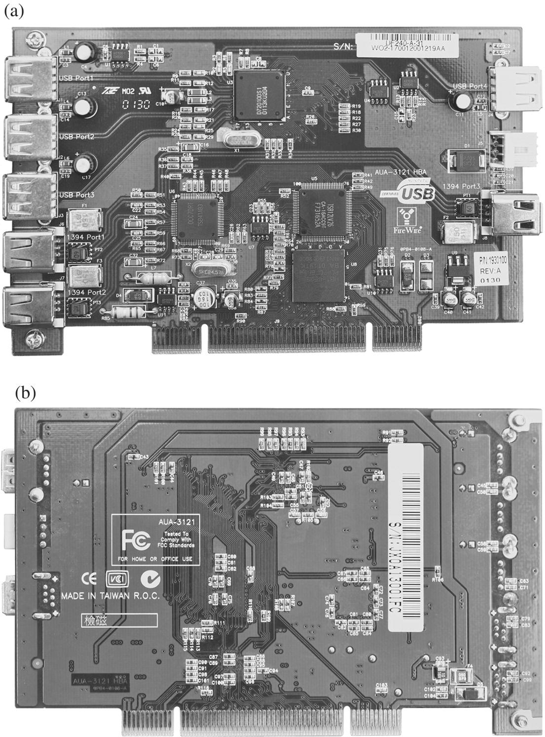
Figure 6.2 Example of a printed wiring board (a) top view (b) bottom view. Photo courtesy of A. G. Blum.
For PWB design for reliability, the key considerations are the stress–strength relationships germane to each of
- the board material,
- the electronic and mechanical components themselves, and
- the solder attachments.
There may also be mechanical attachments, like fasteners, especially for large components (transformers, backplane connectors, etc.). If these are torqued to proper values4 during assembly, they will not be a cause of failure later on. The design for reliability implication is that these torque values need to be known to the assembly designer, which again points to the need for adequate information supporting DFR.
6.5.1.1 PWB design for reliability: board material
Torsional and bending stresses are placed on the PWB substrate in normal operation. The relevant strength is the PWB substrate material and thickness. These should be chosen so that cracks, breakage, trace delamination, or other related failures do not occur over the intended service life of the equipment [24]. PWB substrate material should be covered by the same component sourcing management program that is used for other components. See Section “Early life failures”.
6.5.1.2 PWB design for reliability: assemblies of electronic and mechanical components
Following the model for component reliability discussed in Section 3.3.4.4, we may approach design for reliability in assemblies using electronic and mechanical components by addressing each of the three lifetime phases individually. To recall, these three phases are
- early life failures caused primarily by failure of components having defects introduced during their manufacture,
- mid-life failures caused primarily by overstresses applied to otherwise “normal” components (i.e., ones manufactured according to their design intent and containing no manufacturing-introduced defects), and
- end-of-life failures caused primarily by wearout failure modes.
Early life failures
In the “standard model” of component failure (Section 3.3.4.4), the so-called early life or “infant mortality” failures are caused by defects introduced into components during their manufacture. Components having these defects cause their strength to be less than the majority of the population of components not having manufacturing defects. If we were to draw the strength density for this population at time 0, it would be bimodal: most of the components in the population have strength clustering around the larger mode, and some of the population (those with manufacturing defects) clustering around the smaller mode. For example, a metal oxide semiconductor (MOS) requires an oxide of a specified thickness. If the oxide in a particular device is thinner than specified, that device may fail when subjected to “normal” voltage stresses that an oxide of the specified thickness may easily be able to withstand. If some devices with this defect escape the manufacturer’s process controls and make their way into the population of devices sold to users, the users will suffer these “premature” failures.
This model postulates that most of the components in the population that have manufacturing defects eventually will have failed and are no longer in use. When the mechanism is as described in the model, these failures should happen relatively rapidly and the time by which all (or most) of the defective devices have failed should be relatively short. The key to managing the number of early life failures, given this understanding, is to ensure that components are sourced from reputable suppliers who practice systematic quality engineering with effective process controls. Economics usually dictates that reliability testing and “burn-in” of sourced components before assembly is impractical except in some high-consequence systems like nuclear weapons, nuclear power plants, satellites, undersea cable telecom systems, etc.5 The details of supplier management programs for component reliability are beyond the scope of this book. A good place to start exploring these programs is the American Society for Quality publications [7, 30].
Overstress failures
For components in the “normal” part of the strength distribution, most failures are caused by occasional imposition of stresses beyond their strength. Consequently, the key design for reliability principle applicable to prevent component failures in this phase is to ensure that stresses in excess of the components’ strengths are not applied in routine operation.6 For instance, the voltage rating of a capacitor selected for a particular circuit application should always exceed (usually by a factor of at least 2) the voltage that exists in the circuit at that point. To apply similar reasoning to all the components on the PWB would require that the relevant stresses impinging on each of the components be discernible. Table 6.1 lists some important electrical and mechanical components included on many PWBs and the primary stresses that cause failure for each.
Table 6.1 Components and Stresses
| Component | Primary Failure-Causing Stresses |
| Capacitor | Voltage |
| Resistor | Dissipated power |
| Inductor | Current |
| Electromechanical relay | Contact current |
| Semiconductor | Reverse voltage, forward current |
It is still possible that extraordinary overstresses may reach circuits because of exogenous shocks like lightning strikes, power surges, cosmic rays, etc.; and depending on the economics, systems engineers may choose to adopt requirements that force designs to be more resistant to these known stressors. It is rare that a stress that cannot be shielded against; the determination of how much preventive action should be taken to protect against known stresses is a matter for reliability economics and risk management [3, 11, 34]. There is also a significant issue with unanticipated stresses. Design for reliability is necessarily an attempt to forecast the future and, therefore, has better or worse outcomes depending on the tools and information available (see Section 6.4.1) and the abilities of the people who use them, so beyond the standard catalog of known stresses there may be stresses that simply were not anticipated, perhaps because of a not-yet-fully understood new technology application or an unanticipated customer environment. The conventional advice for dealing with unknowns of this kind is to allow more margin in the stress–strength analysis where it is possible to do so reasonably. Implementing this advice requires knowledge of stresses and strengths: what is the current state of the design with respect to known stresses, and how much risk are suppliers and customers willing to assume regarding unknown stresses.
The catalog of stresses affecting electronic components on PWBs includes, but is not necessarily limited to,
- heat, including thermal cycling,
- power dissipation,
- voltage,
- electrostatic discharge,
- current,
- humidity,
- shock, and
- vibration.
Quantitative models for the effect on reliability of at least some of these are found in Section 3.3.5. The design for reliability idea here is to enable designers to use these models in a convenient way during schematic capture (PWB electrical design) and PWB layout (PWB physical design) to ensure that the circuit and physical designs do not present overstresses to components. In particular, a design for reliability procedure for PWBs must identify the stresses on the components in the current iteration of the PWB design, identify those that are overstresses, and offer the designer options by which those overstresses can be reduced or removed. In this section, we describe the basic outline of a procedure of this kind that covers thermal and electrical stresses.
Requirements tip: Refer to the component reliability model discussed in Section 3.3.4.4. The idea underlying the PWB design for reliability procedure is that the components on the PWB have reached the constant hazard rate period of their lifetimes, for this is where the influence of randomly occurring overstresses on hazard rate is postulated to occur (see Exercise 1 of Chapter 3). Therefore, effective use of this tool requires that a component acquisition management program be implemented for the purpose of eliminating from the incoming population of components any that may have manufacturing defects and may be subject to early life failure. The postulate of the model that components have not yet reached their end-of-life phase is also to be respected when using this procedure. Reliability requirements should be constructed with this in mind when designing PWBs for reliability using this procedure.
Two main ideas underlie this technology:
- Include electrical and thermal stresses in the analysis.
- Integrate the procedure with the computer-aided design process.
These requirements determine what analyses and information will be needed and how they should be interconnected. Electrical stresses (voltage, current, and power dissipation) are discernible from circuit simulation. Once the power dissipated by each component is known, a thermal analysis can be run to determine the distribution of heat across the PWB and find the temperature of each component on the PWB. Once the temperature and electrical stress for a component are known, its reliability may be estimated from an accelerated life model or other appropriate stress-life model (Section 3.3.5). Figure 6.3 shows a schematic of the analyses, databases, and their interconnections (information flows) that can be used to construct a design for reliability procedure for PWBs.
Figure 6.3 Design for reliability procedure for PWBs.
The thermal impedances for each power-dissipating component needed by the thermal analysis tool can be stored in the reliability database or some other database accessible to the thermal analysis program. The schematic capture and physical layout analyses are typically part of a computer-aided design (CAD) system so the design for reliability procedure easily integrates with CAD, allowing for early insight into potential reliability problems. Based on the PWB reliability estimate output, the designer may select other components to provide greater margin between stress and strength or rearrange the board layout to minimize hot spots and decrease the temperature on sensitive components. These changes should result in improved PWB reliability. The use of this type of design for reliability procedure is consistent with the idea of incorporating reliability engineering considerations into the system design from the earliest possible moment.
A brief summary of operation of the procedure follows. Once schematic capture is complete, circuit simulation may be run with whatever inputs come from elsewhere in the system. While the primary purpose of circuit simulation is to gain greater understanding of the circuit’s performance against its functional requirements, for purposes of this procedure it is used to also develop voltages, currents, and power dissipations pertinent to each component. Voltages and currents combine with stress-life models (Section 3.3.5) to yield reliability estimates for those components. Power dissipations are combined with ambient temperature and thermal impedances to determine individual component temperatures that serve as inputs to thermal analysis of the entire PWB. Thermal analysis is typically a finite element approximate solution of the heat equation on the PWB using the component temperatures as sources; it produces a thermal profile of the entire PWB so that potential overheating of neighboring components may be detected and remedied by rearrangement of the circuit layout on the PWB. While component reliability estimates resulting from this analysis are important for a reliability model for the entire PWB, an equally important purpose of the procedure is to highlight components that may be overstressed because of circuit design, component selection, and/or physical layout. The design for reliability aspect of this work is that it enables these overstresses to be detected early in the design process when changes to remove the overstresses can be made with minimal disruption.
End-of-life failures
It is particularly important to avoid end-of-life failures because the increasing hazard rate characteristic of those failures means that a many failures may accumulate with increasing frequency over a population of installed systems. While this is a statement about a population of nonrepairable items, a system whose life distribution is increasing and which is repaired according to the revival protocol will experience an increasing failure intensity (Section 4.4.3) (Ascher and Feingold’s “sad system” [1]; see Exercises 2 and 3).
For electronic components, a strategy that is often used is to select components so that, with the stresses applied by the circuit, the end-of-life (increasing hazard rate) period does not begin until after the service life of the system is over. This strategy is one of the foundations of the life distribution model described in Ref. 21; see also Section 3.3.4.4. This strategy is effective when it is possible to use it. Sometimes, new or unproven technology must be used in a cutting-edge system, and it is still necessary to protect against the risk of premature activation of a wearout failure mode. The AT&T SL-280 undersea fiber-optic cable communication system used optical transmitters containing laser diodes that had a known wearout failure mode [32]. To meet a very demanding system reliability requirement of no more than three failures in 25 years of operation, it was necessary to provide cold standby redundancy: for each laser transmitter in the system, three cold standby spares were provided along with an innovative optical relay switching system that enabled the spares to be inserted into the optical path as needed. This example illustrates the value of an appropriate redundancy strategy as a means for dealing with known wearout failure modes. See Chapter 7.
For mechanical components, in addition to (or instead of) these two approaches, there is the possibility of preventive maintenance. A good example of this is the internal combustion engine. Auto manufacturers recommend a schedule of engine oil changes to guard against two wearout failure mechanisms: first, unlubricated or poorly lubricated sliding friction of piston rings against cylinder walls and bearings against journals produces mechanical wear; second, engine oil deteriorates in use and its lubricating properties diminish. So far, no one has invented an engine oil whose wearout mechanism (physical/chemical deterioration) does not activate until after the vehicle’s service life (potentially, many hundreds of thousands of miles) is over, so renewing the oil periodically is the only sensible preventive maintenance option. Doing so also forestalls the sliding friction wearout failure mode in the cylinders and bearings.
6.5.1.3 PWB design for reliability: solder attachments
The through-hole and surface-mount components are attached to the copper circuit traces on the PCB with solder, usually using a wave-soldering machine. Therefore, in addition to managing the reliability of components on the PWB, it is also necessary to manage the reliability of the solder connections. The major factors contributing to solder connection failure are
- defective solder joints (e.g., “cold” solder joints),
- thermal cycling, and
- shock and vibration.
The incidence of defective solder joints introduced during manufacturing is minimized through use of appropriate process controls. The degree of susceptibility of solder joints to thermal cycling, shock, and vibration depends on the solder material (usually an alloy of tin, lead, bismuth, antimony, etc.) and the shape and size of the solder joint. Solder attachment reliability has been widely studied [15, 16], but new materials are constantly being developed, especially in response to recent reduction of hazardous substances (RoHS) regulations. A thorough design for reliability process for PWBs should incorporate the latest understanding of the solder attachment system used.
6.5.2 Design for Reliability in Complex Systems
At higher levels of assembly, other factors besides component failures contribute to system failures and outages. These may include unanticipated interactions (i.e., timing mismatches in digital circuits) between or among subassemblies, connector and cable failures, operator errors, software faults, etc. Good design for reliability endeavors to anticipate as many of these factors as possible and to design the system so that consequent failures are minimized, and properly managed when they do occur. Quantitative system reliability modeling is useful in this task, and should be undertaken with the motivation of using it to discover weak spots in the design which then can be strengthened (within the economic constraints that prevail) so that reliability requirements will be met.
It is possible to use mathematical optimization techniques to help design for reliability in complex systems, either by minimizing cost subject to a reliability requirement (used as a constraint), or by maximizing reliability within a given cost constraint. The literature on these techniques is found under the topic of “reliability optimization” and is extensive. Important studies that may be used as a starting-off point in this literature include but are not necessarily limited to Refs. 10, 27. In practical reliability engineering applications, these methods can often provide qualitative insight, especially with regard to architecture selection (redundancy), but rarely can they provide specific design solutions. The methods require information about the cost and reliability of all design alternatives, such as LRU architecture and design. There is not usually a continuum of reliability versus cost in components or entire LRUs. Most often, there may be only a few components that may be suitable for a particular application, which implies that the reliability/cost function for those components is discrete. For example, in decades past, integrated circuits (ICs) were manufactured in plastic cases for commercial applications and in ceramic, hermetic cases for military applications. The ceramic-packaged ICs were considerably more expensive than the corresponding commercial versions, and while their reliability was commonly assumed to be better than the plastic-packaged versions, later understanding determined this not to be so, and the manufacture of ceramic-packaged ICs was discontinued. Nonetheless, the point of the example is that, for these ICs, there were only two choices available to the designer: two reliabilities and two corresponding costs. A continuum of reliabilities and costs did not exist for these parts, and reliability optimization studies became straightforward (choice between two alternatives) or impossible (for the lack of a continuum of costs and reliabilities).
All is not lost, however. Design for reliability for complex systems is facilitated by two qualitative techniques that have found wide applicability and good success over many kinds of systems, including high-consequence systems like nuclear power plants (Chapter 7). The next section discusses FTA and failure modes, effects, and criticality analysis (FMECA) techniques that can be applied at any stage in design but, as always, are recommended for use as soon as possible after the design concept has been established.
6.6 QUALITATIVE DESIGN FOR RELIABILITY TECHNIQUES
In this section, we introduce two techniques for anticipating and managing failures. FTA and FMECA help the systems engineer catalog the possible failure modes in a system or service, understand how the user may use or misuse the system and how such use or misuse can contribute to system failures, and assess whether proposed countermeasures will be cost-effective as well as effective in preventing failures.
6.6.1 Fault Tree Analysis
6.6.1.1 Introduction
FTA is a disciplined approach to discovering the failure mechanisms and failure causes associated with a failure mode. It is a form of the root cause analysis practiced in quality engineering. It is often referred to as a “top-down” approach because the starting point of an FTA is a system failure, a negative result we wish to avoid to the extent possible within the economics of the system or service. This requirements violation is pictured as the root event of a tree diagram and is referred to as the “top event” in the tree. The analysis proceeds by diagramming as branches emanating from an event the causes of each event in the tree, starting at the top event and working down the tree. The Boolean operators “and,” “or,” and “not” are used when there are multiple causes for an event. Page connectors are used when it is desirable to divide the diagram into smaller pieces for clarity or to fit to available space. The root cause analysis continues until it reaches a stage where it is possible to identify a reasonable countermeasure for the event at that stage. The reasoning is then that preventing the events at the “bottom” of the tree prevents the occurrence of all the undesirable events above it in the tree, including the final “top event” that represents system failure. Usually, some code or abbreviation is employed in the diagram to identify the events without having to take up space by writing out their entire description in the limited space available in the diagram. FTA, therefore, is a deductive approach to root cause analysis, supported by a simple graphical representation of a hierarchy of causes. Its aim is to find, for each system failure mode studied, a primitive cause or causes that can be prevented through identifiable actions.
A fault tree as we have described it is oriented toward negative outcomes, or failures, and the causal relationships between them. The top event is a violation of some system requirement. A thorough design for reliability analysis can be conducted systematically by cycling through all the system requirements and starting a fault tree for each identifiable violation. This is likely to result in an enormous amount of work and only rarely is so comprehensive a fault tree study conducted. The exceptions are cases where the consequences of failure are catastrophic, such as in a nuclear power plant, or where repair is not possible while a long useful life is desired, such as for a satellite. One can also conduct a similar analysis using successes instead of failures. In this analysis, the tree is oriented toward positive outcomes and the causal relationships between them. For each requirement, a top event can be formed as a successful operation according to the requirement, and the contributing events are events that cause proper operation rather than failure. Such an analysis might more properly be called a “success tree analysis.” The success tree is less adapted for design for reliability because the very events that you need to uncover—namely, those involving failures and their causes—are left implicit in the success tree. So the choice between an FTA and a success tree analysis is not only a question of volume (if there are many ways in which a requirement can be violated but only a few in which it is fulfilled, a success tree analysis might be less time-consuming, and conversely). Most reliability engineering specialists use FTA, but you should be aware that alternatives exist.
FTA also may be used quantitatively to find the probability of occurrence of the top event if reasonable probabilities can be assigned to each of the primitive, or root, causes. The explicit use of Boolean operators in the tree allows direct application of the calculus of probabilities to “roll up” the probabilities from the lowest level of the tree to the top event. Usually, all the required independence and disjointness properties of the events in the tree are assumed, but this should always be examined. Sometimes, a fault tree will contain multiple connections between branches or the same event may appear in more than one place in the tree. In these cases, simple calculus of probabilities is not adequate to obtain the probability of the top event. A cut-set analysis (Section 6.6.1.3) is used instead.
Before we undertake a more detailed description of FTA, let’s consider a small example.
6.6.1.2 Example: passenger elevator fault tree
For a passenger elevator, the occurrence of a free fall of the elevator car is a serious event with the potential for serious injuries or loss of life. Presumably, there is a safety requirement stating that the elevator car is not to fall freely at any time under any conditions. To illustrate how FTA works, we build a fault tree for the top event “Elevator car falls freely.” To construct a fault tree for this event, we need to know something about how an elevator operates, so the next few paragraphs provide a brief description of passenger elevator operation. This description is sketchy and incomplete but provides enough information so that the principles involved in construction of a fault tree can be discerned. A realistic fault tree for a real passenger elevator installation will necessarily be more detailed and comprehensive. Do not mistake this simple illustration for a fault tree that is thorough enough to be used for a real elevator installation.
The three primary assemblies that affect the elevator operation are the control unit, the drive and suspension unit, and the brake unit. The control unit contains a microprocessor that responds to users’ signals to move to a desired floor. The control unit starts the drive unit that moves the car to the desired floor and opens the entry doors when the car has come to a stop. The control unit also receives signals from switches in the elevator shaft so that it knows where the car is at all times. The drive and suspension unit holds the car suspended in the shaft and moves the car in response to signals from the control unit. The drive and suspension unit is supposed to be inactive (i.e., the car should not move) unless a signal is received from the control unit. The brake unit operates on the motor in the drive and suspension unit to hold the car motionless when power is removed from the motor and to allow the motor to turn when power is applied to it.
We recognize that there are three possible causes for the car to fall freely: the system does not hold the car, the suspension cable breaks, or the suspension cable slips off its pulley. Label the top event “1” and the causing events as “2,” “3,” and “4,” respectively. Then Figure 6.4 is the start of the fault tree.

Figure 6.4 Beginning a fault tree for passenger elevator example.
In Figure 6.4, the top event “1” and event “2” are drawn as rectangles, indicating that they will be further analyzed to discover their more basic causes. The diamond-shaped boxes indicate events that will not be further analyzed. These are considered to be root causes for which effective countermeasures can be applied. An “or” connector is used to indicate that if any of events “2,” “3,” or “4” occurs then the top event occurs. It may be possible to further decompose events 2 and 3 into root causes, but we shall not do so in this simple example. Again, the decision to seek deeper root causes rests on whether effective countermeasures can be devised for the event(s) at the bottom of the diagram. In this example, for instance, determining how to prevent the suspension cable from breaking may require additional information about the causes of a cable break.
We may now look for causes of event “2,” the system does not hold the car. Two things have to take place for the system to not hold the car when the suspension cable is not broken or off the pulley: the brake fails (“5”) and the motor turns freely (“6”). We identify three causes for “brake fails”: loss of friction material (“7”), the brake solenoid sticks in the “brake off” position (“8”), or the control unit erroneously disengages the brake (“9”). There are two causes for the motor to turn freely: either there is no power to the motor (“10”), or the motor has failed (“11”). These events and their causes are diagrammed in Figure 6.5.
Figure 6.5 Sub fault tree for “system does not hold car” event.
Note that each of the three causes of lack of braking is considered sufficiently analyzed (at least for purposes of this simple example) that countermeasures may reasonably be applied to them. In a real FTA for this system, it would be necessary to identify further root causes for event 7, such as improper preventive maintenance allowing the brake linings to wear beyond a safe point.
Loss of power to the motor may be caused by either the controller erroneously turning off power to the motor (“12”) or by a total loss of system power (“13”). The erroneous behavior of the controller may be caused by a hardware failure (“14”) or a software failure (“15”). These events and their causes are shown in Figure 6.6. Again, in a realistic FTA, the events 14 and 15 would most likely be analyzed further because “hardware failure” and “software failure” are not specific enough to be able to apply reasonable countermeasures.
Figure 6.6 Sub fault tree for “no power to motor” event.
We may include estimates of the probabilities for each of the elementary events (those in the diamond-shaped boxes) and use the calculus of probabilities to obtain an estimate of the probability of the top event. The elementary events are 3, 4, 7, 8, 9, 11, 13, 14, and 15. Let pi denote the probabilities of the events in the tree, i = 1, . . ., 15. Then the probabilities of the events in the tree are as follows:
- p12 = p14p15
- p10 = p12 + p13
- p6 = p10 + p11
- p5 = p7 + p8 + p9
- p2 = p5p6
- p1 = p2 + p3 + p4.
The probability of the top event, written in terms only of the probabilities of the elementary events, is, finally, p1 = (p7 + p8 + p9)(p14 p15 + p13 + p11) + p3 + p4. Of course, to write the probability of the top event (and the intermediate events) in this way, we need to assume that all events entering an “and” gate are stochastically independent, and all events entering an “or” gate are disjoint. In general, this will not be true and evaluation of the probability of the top event cannot be done with the ordinary calculus of probabilities. A useful alternative is provided by the method of cuts.
6.6.1.3 Cuts and minimal cuts in fault trees
Calculating the probability of the top event in a fault tree is often more complicated than shown in the earlier example because the same event may appear in different branches of the tree. This is a reflection of the fact that the same event may be the cause of several different effects. For example, consider the following modification of the fault tree in Figure 6.6.
Here, the top event can be caused by either event A or event B. C and D act together to cause event A, and C and E act together to cause event B. Let the probabilities of these events be pA, . . ., pE. Then the probability of the top event is

Notice how the repeated appearance of event C requires reduction of the intersection in the second line. This phenomenon appears frequently in realistic fault trees. Most realistic fault trees are more complicated than this example, so a simpler means of computation is desirable.
The use of paths, minimal paths, cuts, and minimal cuts to model system reliability was introduced in Section 3.4.7. The key idea was that for reliability block diagrams, especially those not having a series-parallel structure, another approach to developing an expression for the system reliability is offered by the method of paths and cuts. The cut technique is well adapted to the computation of the top event probability in a fault tree. To illustrate the use of cut-set methods in fault trees, we will list the cuts and minimal cuts in the passenger elevator fault tree example in Section 6.6.1.2.
Recall that a cut in a graph is a set of nodes and links whose removal from the graph causes the graph to become disconnected. In the fault tree case, the links serve only as connectors and may be disregarded. Two useful rules for cuts in fault trees are
- if some events are connected to a higher event by an AND gate, only one of those events need be part of a cut containing the higher level event and
- if some events are connected to a higher event by an OR gate, all those events need to be part of a cut containing the higher level event.
For example, in Figure 6.7, the cuts are {A, C, B, C}, {A, C, B, E}, {A, D, B, C}, {A, D, B, E}, {A, C, E}, {A, D, E}, {B, C, D}, {B, D, E}, {C, D}, {C, E}, {D, E}, and {C}. The minimal cuts are {C} and {D, E}, so the minimal cut set is {{C}, {D, E}}. Following the reasoning of Section 3.4.7, the probability that the fault tree fails to function (i.e., the top event does NOT occur) is given by the probability of the tree’s minimal cut set. Repeating: in the case of a fault tree, “the system (the fault tree) fails” means “the top event does not occur” because the “system” in this case is “successful occurrence of the top event.” As in Chapter 3, we (ab)use the same letter for the event and for the indicator that the event occurs, so the probability that the top event does not occur is P({C = 0} or {D = 0 and E = 0}). Using pC = 1 – P{C = 0} = 1 – P(~C), etc., we obtain


Figure 6.7 Fault tree illustration with a repeated event.
which is the same as the expression following Figure 6.7. Note the confusion that can easily occur here. The top event is one of the failure modes of the original system, that is, a system failure. Using the cut-set reasoning, our target is the top event NOT occurring, that is, the “system” represented by the fault tree fails. In other words, “failure of the fault tree ‘system’ ” means “the top event does not occur,” which is equivalent to saying “the (original) system7 does not fail.” Fortunately, these difficulties occur mainly when constructing a fault tree by hand and are obviated by the availability of many software packages for fault tree construction and analysis (one of the earliest of these is [40]; since then, many professional fault tree packages have appeared in the commercial marketplace).
We close with the observation that the minimal cut set is the catalog of actions that can be taken to forestall or prevent the top event (system failure when so defined) from occurring. For example, in Figure 6.7, if you can prevent C from happening, or if you can prevent both D and E from happening, then the top event does not occur. In this way, a useful by-product of fault tree construction is a simple procedure for cataloguing countermeasures.
6.6.1.4 Application: system reliability budget
We began a discussion of reliability budgeting in Section 4.7.3 in which a solution based on mathematical optimization was proposed. Sometimes, it may not be possible or desirable to develop a formal reliability budget using the optimization ideas shown there. But it is still a best practice to create a reliability budget so that all development teams know what reliability targets they need to reach. For a more informal approach to reliability budgeting, consider that an FTA can be a viable approach. To do this, the elements of the fault tree need to correspond to the items that will appear in the reliability budget. A fault tree approach provides additional flexibility in that the elements of the fault tree need not be subassemblies or subsystems only, but may also be events of significance to system reliability. To use this approach, assign probabilities (or life distributions, availabilities, etc., as appropriate) to each element of the tree and use the standard fault tree computation to determine the appropriate reliability effectiveness criterion or figure of merit for the system. If the tree is small enough, trial and error may work well. For larger trees, one would need to link the output of the fault tree construction software to the input of a budgeting optimization routine.
6.6.2 Failure Modes, Effects, and Criticality Analysis
FTA provides a systematic way of discovering the causes of system failures. Its premise is that, starting with a list of system failure modes, which comes from reviewing the system’s attribute requirements and cataloguing the different ways they can be violated, reasoning can be applied to discern the intermediate and root causes of these system failures. The results are displayed in a tree diagram with the system failure as the top (root) node and the intermediate and root causes branching from that, with the links indicating causality relationships. FMEA, by contrast, provides a systematic way of discovering the consequences of failures of parts of the system. It begins by postulating failures of parts of the system and determines the consequences of those failures in a sequence whose terminus is a system failure. So in a sense, FMEA is an opposite, or complementary, reasoning process to that of FTA. The most common graphical display of FMEA results is as a table or spreadsheet as illustrated in the next section.
Language tip: Note that the use of “failure” in FMEA is different from that in FTA. In FTA, “failure” refers to system failure, violation of a system requirement. FMEA, by contrast, concerns failures of components of a system and how the effects of these failures propagate throughout the system to cause (one or more) system failure(s).
Language tip: In this book, we will use the acronym FMECA to mean FMEA with the criticality component, FMEA to mean failure modes and effects analysis specifically excluding the criticality component, and FME(C)A to indicate either FMEA or FMECA generically.
Requirements tip: To know what “failure” means for system components, we need to know the requirements for those components. For simple components like resistors, bearings, and the like, these requirements are usually limited to operation of the component within its specified parameters. For example, a resistor may be required to have a resistance value of between 950 and 1050 Ω and to be able to dissipate 0.25 W of power. A resistor with these parameter values is selected for use in a system if these values allow it to perform its circuit function(s) in the system. Usually, no additional requirements for isolated, single components like these are imposed. FME(C)A asks what are the consequences for circuit operation if the resistor no longer meets these specifications. More complex subassemblies may have additional or more functional requirements; in the FME(C)A context, failure of a subassembly means violation of one or more of these.
6.6.2.1 Failure modes and effects analysis
We begin by examining FMEA, a purely qualitative technique. We discuss two types of FMEA: concept FMEA which is suitable for use early in the design of a system, before any specific hardware or software have been specified, and design FMEA which captures the additional detail that is beneficial when the design is more complete. Section 6.6.2.2 adds a quantitative dimension to FMEA by incorporating the notion of criticality as a way of ranking the importance of the failures studied.
Concept FMEA
Concept FMEA is useful first at the stage of a design where it is possible to identify a system functional decomposition and the major design elements that will fulfill the identified functions. The system functional decomposition is a good place to begin a concept FMEA because constituent elements of the system are identified in the functional decomposition and the FMEA reasoning process can begin with these elements. The FMEA reasoning is a process of inquiring for the consequences of failures, and the consequences of those consequences, etc., continuing until a system failure is identified as a final consequence of a chain of failures beginning with the system’s components or subassemblies. Concept FMEA begins by postulating failure of one of the system’s functional elements and listing the consequences of that failure. Each of those consequences, in turn is subjected to the same reasoning. The effect of a failure of an element of the system could be the cause of failure of another element of the system, etc. The process stops when a chain of consequences, or failures, ends at a system failure. The design for reliability aspect is that preventing the first element failure in the chain prevents the others, and the consequent system failure.
Example: Concept FMEA for a home alarm system. A home alarm system typically includes these features:
- Intrusion detection,
- Carbon monoxide,
- Smoke detection,
- Alerting of a central monitoring facility when an alarm event (unauthorized access, excess CO, smoke/fire, etc.) takes place,
- Battery backup during periods of AC power failure, and
- Facility for user-initiated testing.
It contains a sensor for each location where access is possible (usually doors and first-floor windows), carbon monoxide and smoke detectors, connection to a telephone line, a local CPU, and a control panel. A functional decomposition for a (generic) home alarm system could be developed (see Figure 6.8).
Figure 6.8 Home alarm system functional decomposition.
AD-1 through AD-n are the access detection switches. The system can be in any of three states at any time: armed, ready-to-arm, and failed. Concept FMEA can begin with the blocks in the functional decomposition. Table 6.2 aids in completing a concept FMEA for this example.
Table 6.2 Concept FMEA Table
| Item | Function | Failure Mode | Failure Cause(s) | Effect of Failure |
| 1 | CPU | PWB failure | Component failure | System totally inoperative |
| Solder attachment failure | ||||
| Power surge | ||||
| 2 | Telephone dialer | Does not detect dial tone | Loose or broken telephone line connection | Cannot dial out to alarm HQ |
| Does not generate DTMF tone(s) | Solder attachment failure | |||
| Component failure | ||||
| 3 | Access detector | False positive | Defective switch (short) | False intrusion alarm |
| False negative | Defective or dirty switch (open) | Alarm event missed | ||
| 4 | CO detector | False positive | Defective component, CO sensor element, or solder attachment, or other circuit failure | False CO alarm |
| False negative | Missed CO event, possible loss of life | |||
| 5 | Smoke detector | False positive | Defective component, smoke sensor element, or solder attachment, or other circuit failure | False fire alarm |
| False negative | Missed fire event, possible property damage or loss of life | |||
| 6 | Control panel | Does not respond to inputs | Defective keypad | Alarm system inoperative |
| Illumination failure | LED failure | Difficult to use in the dark | ||
| 7 | Power | No power to system | AC power and backup battery failures | System totally inoperative |
Obviously, this example is far from complete. Other failure modes are not included; some failure causes are not specific, etc. The purpose of this example is not to provide a complete or generic concept FMEA for a home alarm system. Rather, it is to illustrate the reasoning process that is used to complete the table. The completeness of the system functional decomposition determines to a great extent the quality of a concept FMEA. It is good practice to include each block in the system functional decomposition in a concept FMEA.
Design FMEA
The distinction between concept FMEA and design FMEA is that design FMEA can be more detailed, and therefore more specifically helpful for design for reliability, because more of the design is committed. Specific hardware and software have been identified that will perform the functions in the system. In other words, the functional blocks in the system functional decomposition are fleshed out with specific hardware and software to perform the functions. Design FMEA can begin with more specific system component information and so promotes more effective design for reliability. Specific design for reliability decisions can be taken on the basis of design FMEA. For instance, the functional decomposition for a domestic forced-air heating system will contain a block for “air impeller.” A concept FMEA explores the consequences of air impeller failure. Design FMEA can be undertaken when a specific blower motor and fan model is chosen; the failure characteristics of that motor and fan model add understanding to the concept FMEA and allow the system designer to decide whether this specific blower motor model is appropriate for use in the system.
Table 6.3 illustrates a design FMEA for the CO detector in the home alarm system discussed in Section “Concept FMEA”.
Table 6.3 Design FMEA Example
| Item | Function | Failure Mode | Failure Cause(s) | Effect of Failure |
| 1 | Connector | Open | Corrosion, improper assembly, not correctly seated | Excess CO may not be alarmed, possible loss of life |
| Short | Improper assembly | CPU sees CO detector as defective | ||
| 2 | CO sensor element | Open | Broken lead due to improper assembly | Cannot detect excess CO, possible loss of life |
| Short | Manufacturing defect | False CO alarm | ||
| Oversensitive | ||||
| Undersensitive | Accumulation of dirt, corrosion, manufacturing defect | Cannot detect excess CO, possible loss of life | ||
| 3 | CO detector circuit | False positive | Component or solder attachment failure | False CO alarm |
| False negative | Excess CO may not be alarmed, possible loss of life | |||
| 4 | Wiring to CPU | Open | Improper initial assembly, damage from vermin | Missed CO event, possible loss of life |
| Short | Defective insulation | CPU sees CO detector as defective |
Again, this design FMEA is incomplete. It would normally be executed for a specific CO detector circuit and failure causes could therefore be more specifically identified. Circuit simulation would provide an indication of how the distribution of sourced component values and drift of component values over time may affect operation of the detector when new and as it ages. Specific countermeasures could then be devised and their economics evaluated. This is the value of design FMEA in design for reliability.
Design FMEA is related to robust design (Section 6.8). Some of the same tools are used. For example, circuit simulation is used not only to determine requirements for individual circuit elements but also to help understand how operation of the circuit outside its specification limits may contribute to failures further up the design hierarchy.
6.6.2.2 Failure modes, effects, and criticality analysis
FMECA adds a quantitative component, criticality, to FMEA. Criticality is a number attached to each outcome of the chain of causality. Criticality, also called risk priority number (RPN), is arrived at by multiplying three numbers:
- Probability of occurrence of the failure,
- Severity of the failure, and
- Probability that the failure will affect the customer/user.
Unless a detailed reliability model for the system exists, the probability of occurrence of the failure is subjectively assessed. A 1–10 scale is commonly used in accordance with the Table 6.4.
Table 6.4 Example of a FME(C)A Probability Scale
| Scale Quantity (Rank) | Qualitative Criteria | Failure Occurrence | |
| per 100,000 Units | per Year | ||
| 1 | Remote possibility of occurrence | Negligible | |
| Unreasonable to expect that failure would occur | |||
| 2 | Relatively low likelihood of occurrence. Failure would be surprising | 5 | 1/3 |
| 3 | 10 | 1 (annually) | |
| 4 | Moderate likelihood of failure; occasional failure but not in major numbers | 50 | 2 (biannually) |
| 5 | 100 | 4 (quarterly) | |
| 6 | 500 | 12 (monthly) | |
| 7 | High likelihood of failure; comparable to products/processes that have caused problems before | 1,000 | 52 (weekly) |
| 8 | 5,000 | 365 (daily) | |
| 9 | Very high likelihood of failure, almost certain that many failures will occur | 10,000 | 10,000 (hourly) |
| 10 | 50,000 | 40,000 | |
Table 6.4 provides an illustration of a possible FMECA probability scale. The values and criteria shown are not universal; other probability scales are sometimes used. The scale is somewhat arbitrary and other choices also make sense because FMECA aims to provide a relative ranking of failures rather than an absolute measurement of failure impact. At the stage of development at which FMECA is normally used, it is usually not possible to be very precise about these probabilities. A good deal of subjective judgment, based on experience, is used. The absolute values of the criticalities or risk priority numbers are not, and are not intended to be, reliable. The relative ranking of these is used to help assess which failures should receive attention first. The output of an FMECA is displayed as a Pareto chart (ordered bar chart) with the risk priority numbers in descending order from left to right. It is possible to tell at a glance the priority in which potential failures should be addressed.
The second component of the risk priority number is the severity of the failure. A scale is imposed on a set of qualitative criteria so that a risk priority number can be developed. Table 6.5 gives an example of a possible severity scale.
Table 6.5 Example of a Severity Scale
| Rank | Qualitative Description |
| 1 | Minor—A failure not serious enough to cause injury, property damage, or system damage, but which will result in unscheduled maintenance or repair |
| 2 | |
| 3 | |
| 4 | Marginal—A failure may cause minor injury, minor property damage, or minor system damage which will result in delay or loss of availability or mission degradation |
| 5 | |
| 6 | |
| 7 | Critical—A failure can cause severe injury, major property damage, or major system damage which will result in mission loss |
| 8 | |
| 9 | Catastrophic—A failure can cause death or complete system loss |
| 10 |
Again, the scale shown is arbitrary, and other similarly useful scales are in common use.
Finally, the third component of the risk priority number is the probability that the failure will be detected before it affects the system user or customer. The reasoning here is that a defect can be detected and prevented from affecting system users should rate lower on a risk priority scale than one that is not prevented and does affect system users. Accordingly, Table 6.6 illustrates a sample user impact scale.
Table 6.6 Sample Scale for Probability of Affecting Users
| Rank | Qualitative Description | Probability of Affecting Users |
| 1 | Remote likelihood that the defect will not be detected before occurrence—it will not affect the user. | 0–0.05 |
| 2 | Low likelihood that the defect will not be detected before occurrence—it will probably not affect the user. | 0.06–0.15 |
| 3 | 0.16–0.25 | |
| 4 | Moderate likelihood that the defect will not be detected before occurrence—it may affect the user. | 0.26–0.35 |
| 5 | 0.36–0.45 | |
| 6 | 0.46–0.55 | |
| 7 | High likelihood that the defect will not be detected before occurrence–it probably will affect the user. | 0.56–0.65 |
| 8 | 0.66–0.75 | |
| 9 | Very high likelihood that the defect will not be detected before occurrence—it will affect the user. | 0.76–0.85 |
| 10 | 0.86–1 |
Sometimes, it is helpful to think of this scale in reverse terms, that is, as a scale measuring how readily the effect may be prevented. Effects for which there is a readily available preventive measure receive lower ranks. Effects for which preventive measures are not available or difficult or expensive to implement receive higher ranks.
The risk priority number resulting from use of these scales is a number from 1 to 1000, the product of the three rank numbers from each of the three factors. The RPN has no absolute meaning, but RPNs provide a relative ranking of the importance of each of the defects considered in the FMECA. The Pareto chart is an effective way to display RPN information, allowing users to discern at a glance the most critical defects.
The fundamental structure of FMECA lends itself readily to incorporation in spreadsheet software. FMEA tables are augmented with four additional columns in which the criticality information is displayed. The first three columns contain the rank information from Tables 6.4 to 6.6, and the fourth column contains the RPN, the product of these three numbers.
Other FME(C)A applications
FME(C)A is also effective as a design for reliability tool for less-tangible objects like processes, services, and software. For processes, replace the system functional decomposition with a process flow diagram so that the downstream effects of improper operation of any process step can be determined. For services, the service functional decomposition (Section 3.4.2.3 gives an example; see also Section 8.3) serves the same purpose. An FME(C)A for software is facilitated by data flow and control flow diagrams [13].
6.6.2.3 Summary
FME(C)A and FTA are complementary design for reliability tools. At any block in the system functional decomposition, it is possible to start an FME(C)A or an FTA as long as requirements for that functional block exist. FTA will look from a particular functional block down the design hierarchy, into the supporting blocks, inquiring how failures in those supporting blocks may cause failure in the study block. FME(C)A will look from a particular functional block up the design hierarchy, into the blocks it supports, inquiring how failures in the study block may cause failures in functional blocks it supports. Both points of view are useful. Limited resources may force a choice because of lack of staff or time to carry out both procedures. One important factor influencing the choice is that FTA requires more detailed information about the design than does FME(C)A. A concept FME(C)A can begin earlier in the design process because only the system functional decomposition is needed. To be useful, FTA needs more-detailed information about components and subassemblies of the system and how they operate so that cause and effect may be determined in specific, rather than general, terms.
Many resources are available to help reliability engineers and associated staff carry out FME(C)A studies. Standards include MIL-STD-1629A for the defense industry, SAE J-1739 for the automotive industry, IEC 60812 for the electronics industry, and others. Even though FME(C)A is easily enough automated with simple spreadsheet software, many dedicated software resources for FME(C)A are available in the commercial marketplace.
6.7 DESIGN FOR RELIABILITY FOR SOFTWARE PRODUCTS
Almost every contemporary technological system contains software—lots of software. Many notable failures are caused by software problems. In the past, the primary means for assuring reliability of software-intensive products was through a test, analyze, and fix (TAAF) cycle based on a sequence of development releases that underwent testing and removal of any errors found in that testing. This procedure is depicted schematically in section 6 of Ref. 18 and is the basis for many of the software failure intensity models reviewed in Chapter 9. More recently, it has been recognized that design for reliability can be a more effective means of assuring reliability even in software-intensive products [4, 18]. So the usual procedures we use to design for reliability need to be adapted to the characteristics of software products. In particular, this requires understanding of the failure modes and failure mechanisms peculiar to software products. Section 9.5 discusses failure modes and failure mechanisms for software.
Most system reliability requirements are written in terms of behaviors that are discernible to the user (see Section 9.5.1). As such, it would be unusual for there to be reliability requirements at this level specifically for software. What usually happens is that software contributes one or more causative events at the second level or below of a fault tree. When these cause-and-effect relationships are discerned, system reliability requirements can be allocated to its software component(s). See Section 9.3.1.
Finally, it is important to note that safety and security often come to the fore in discussions of software products. These do not look overtly like reliability issues, but the point of view we adopt in this book is that if a requirement exists for a system, a violation of that requirement is a failure. Even if safety and security requirements are not explicit (and it is a bad idea to leave them as tacit requirements only), most users and customers would regard a system operation that causes injury or loss of life to be a failure. The key idea is that issues like safety and security, even if they do not have explicit requirements, can be treated using the reliability engineering and design for reliability technologies: identify the safety or security failure modes and subject them to the design for reliability process (Section 6.4), use FTA and FME(C)A (Section 6.6) to discover the relevant failure mechanisms, and devise countermeasures tailored to these failure mechanisms. We repeat a point we made in Chapter 1, which is that while the consequences of safety (or security) failures may be more serious than those of other system failures, they may be treated by the same DFR and reliability engineering techniques that we would apply to any other system requirement. In software-intensive products, the constituent materials may be different, but the basic reliability ideas are the same.
6.8 ROBUST DESIGN
The design process yields an “ideal” design in the sense that all design elements (architecture, components, etc.) are abstract until realized in physical space. Any such realization differs from the “ideal” design because of random factors such as component values differing from those specified, drift of component values over time, operating environments differing from those anticipated, and the like. When these random factors are at play, properties of the realized design (and there may be various copies, at least in the case of hardware) differ to some extent from corresponding properties of the “ideal” design. One would like to know in advance whether these potential differences could be significant. The discipline of robust design has grown up to, among other benefits, provide a means for the development team to anticipate the variation in realized versions of the ideal design and adopt corrective measures if necessary. The robust design technology was introduced by Taguchi [37] as a means of improving quality while reducing cost. In this section we will discuss the robust design technology as a reliability-improving activity that prevents failures while avoiding overdesign and decreasing cost.
One of the hallmarks of robust design is the categorization of the factors affecting the operation of the system as control factors and noise factors. Control factors are those that the system development team and system users are able to manipulate to achieve desired effects in a deterministic (or, at least, statistically predictable) fashion. These include design parameter nominal values, material composition, etc. Noise factors are those over which the development team and users have little or no control. They are usually represented as random influences that come from the environment, from the manufacturing process, from variation in design parameters in realization, or from other sources. For instance, while the designer may specify a range of values for a certain component, a physically realized component may still take a random value within (or outside of) that range. Robust design aims to adjust the control factors so that the response of the design to noise factors is minimal, or damped. For instance, a circuit may be designed to have a certain performance. When the circuit is physically realized as a chip or as a PWB with components, the random variation of the chip manufacturing process or of the values of the components on the PWB may cause the performance of the realized circuit to vary from its nominal target.
Robust design is specifically a quality improvement technique. It is not the purpose of this book to conduct a thorough review of the robust design technology. However, it is reasonable to ask whether a design that is robust (little or no response to noise factors) is also reliable, or, to put it another way, can robust design be used as a reliability improvement technique also? The purpose of this section is to show how the notion of drift of design attributes over time unifies robust design and reliability engineering. Paying appropriate attention to these drifts is an important aspect of design for reliability. In brief, the aim of robust design as a design for reliability technique is to maintain a suitably small number of component failures stemming from drift outside specification limits by anticipating the total amount of that drift at the end of the system’s service life and ensuring that this amount of drift can be tolerated by the system [9, 19, 20, 39].
We postulate that certain system attributes drift from their nominal values as time passes. To fix ideas, consider a simple electronic component like a 1000- Ω resistor. Two important ideas are at play here:
- Not every resistor in the population of (nominally) 1000-Ω resistors is exactly 1000 Ω. Rather, the value of a resistor drawn at random from that population has a distribution, usually taken to be approximately normal, with mean 1000 Ω and some standard deviation σ Ω [12].
- As time passes, the values of the resistors in the population change gradually, or drift, so that after the passage of some time the population distribution may retain its original form (i.e., may still be approximately normal) but with a different mean and standard deviation—indeed, in this formalism these are functions of time.
Electronic components, like these resistors, also usually specify a tolerance (1%, 5%, etc.). These tolerance values usually indicate that at least six standard deviations of the component’s value fit within the tolerance percentage. For instance, for a 1000-Ω, 5%-tolerance resistor, this would indicate that 6σ ≤ 100 (=1050 − 950), so we may infer that σ ≤ 16.6 Ω for this population. For higher tolerance components, such as 0.1%, components are sometimes specially selected to fit within the tolerance interval (for 0.1%, this is 999–1001 Ω) and the resulting population is no longer normally distributed. See Exercise 1.
In light of these ideas, the design for reliability actions using robust design are twofold:
- The response (performance) of the circuit at time of manufacture should be evaluated using the distributions of the values of all the circuit elements. This will help determine whether the response of the circuit to this noise factor (e. g., the varying resistance value across the population of resistors) can be satisfactorily damped when the circuit is new. For electronic circuits, this evaluation can be accomplished with a circuit simulation program like SPICE.
- The response of the circuit at future times should be evaluated using knowledge about the drift of the resistance value with time. This will give an idea of how many circuits will have failed by the end of the system’s service life.
For example, consider that a circuit using this resistor will perform satisfactorily if the value of the resistor is between 950 and 1050 Ω. If the population of new resistors is normally distributed with a mean of 1000 Ω and a standard deviation of 30 Ω, then approximately 9.5% of the circuits built will not perform satisfactorily (clearly this is not a realistic example). This situation is illustrated in Figure 6.9.
Figure 6.9 Normal density of resistor values in new population.
To illustrate the notion of drift, suppose that the mean resistor value increases (linearly) at a rate of 10 Ω per year and the standard deviation increases (linearly) at 2 Ω per year. Then after t years, the resistor population has a mean of 1000 + 10t and standard deviation 30 + 2t. After 10 years, the population mean is 1100 Ω and standard deviation is 50 Ω. At that time, 16% of the circuits do not operate satisfactorily. The drift of the resistor values has caused additional circuits to fail.
We turn to a general framework for solving design for reliability problems using the robust design method. The key point is that this technology is appropriate for dealing with failures due to design characteristics drifting over time outside of an acceptable range. To promote consistent use of terminology, we will call the objects in the population “items.” These may be electronic or mechanical components, or subassemblies or entire systems. An item may have one or more failure modes, but at least one of these is of the nature of a drift of a characteristic that, when the characteristic changes enough, causes a failure of the system of which the item is a part. An item is described by one or more characteristics. For example, a resistor is described by its resistance, power dissipation rating, material content, physical size, mounting (leaded or surface-mount), etc. Let X(t, ω) denote for item ω at time t the vector of characteristics whose drift we want to focus on. The notation explicitly allows for this vector to depend on time. Denote by F(x, t) the cumulative distribution function (cdf) of X(t), that is, F(x, t) = P{X(t) ≤ x}, and by f(x, t) the corresponding density function. Suppose that the dimension of X is d and that there is a region A ⊂ Rd that represents the region of acceptable operation for these items. The region A is usually determined by external criteria. For example, a pump may be considered failed when it can no longer pump as much as 60 gph, where the 60 gph requirement comes from the application of the pump in some larger context. Then the proportion of the population that is in the working state (not failed) at time t is
In particular, if we let L(ω) denote the lifetime of item ω, that is, the time it takes for item ω’s characteristics to drift outside of the region of acceptable operation, then
where η represents the lower envelope function
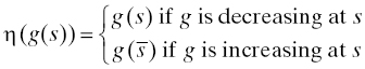
where ![]() is the nearest point to the left of s at which g is decreasing,8 or
is the nearest point to the left of s at which g is decreasing,8 or
Alternatively, η(g) = max{h : h is increasing and h ≤ g}. The use of the lower envelope function means that we do not allow an item whose characteristics have drifted into A to “recover,” or once an item has failed in this fashion, it remains failed. This is consistent with the way a system failure is treated: if drift of an item’s characteristics causes a system failure, remediation of the failure usually begins immediately without waiting to see whether the system heals itself by virtue of the item’s characteristics drifting back into the acceptable region.
Example: Suppose a population of items has a (one-dimensional) characteristic R(t) that has, for each t, a normal distribution with mean 0.2 + 0.002t and standard deviation 0.03 + 0.001t, where t is measured in years. Then we can write R(t) = 0.2 + 0.002t + (0.03 + 0.001t)Z where Z is a random variable having a standard normal distribution. For definiteness, it may help to think of R(t) as the rise times, measured in nanoseconds, of a population of digital integrated circuits. Suppose the failure criterion is that an item is failed if its rise time exceeds 4 ns. Then the lifetime L(ω) of item ω is

The survivor function of L is
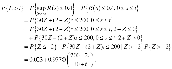
This expression allows us to obtain the value of the life distribution for this population of items at any time t (measured in years). For instance, the probability that the lifetime of an item from this population exceeds 20 years is 0.023 + 0.977Φ(3.2) = 0.023 + 0.997(0.9993) = 0.99932.
Although this example is contrived, it does help point out some useful ideas in the application of the robust design technology to design for reliability. First, distributions of population characteristics can spread (or shrink), as well as shift, as time passes. Second, life distributions derived from this formalism can be defective. For instance, in the example, as t → ∞, 4.5% of the population is still alive. Also, P{L = 0} = 0.977[1 − Φ(20/3)] which is slightly positive.
The robust design technology may be applied more widely in design for reliability than in only the parameter drift scenario. Operational requirements for engineering systems are often written in terms of certain performance parameters such as, for example, the power output of an RF amplifier or the propagation delay across a digital circuit. The value of the performance parameter in any physical realization of the design is influenced by many noise factors. Those that are important for purposes of this engineering technique are
- unit-to-unit variation in system construction,
- unit-to-unit variation in performance of a system’s components and subassemblies,
- drift of physical, electrical, or chemical characteristics of items with time, and
- variation in the environmental conditions in which the systems operate.
In this technology, we postulate that satisfactory system operation requires that the system’s performance parameters remain within some acceptable set of values that we will continue to call A. We consider those failure modes in which performance parameters falling outside this set means that the system has failed. The time of first occurrence of this event is the failure time and the period of satisfactory operation between commencement of system operation and the failure time is the lifetime. We now introduce a formalism that may be used to solve design for reliability and robust design problems of this nature that may incorporate any or all of the four factors listed earlier.
Let X(t, u(t)) denote the vector of system performance parameter values at time t when the environment (the collection of all extrinsic noise factors that influence system performance) is described by a function u(t) of time. u may be modeled as a deterministic function or as a stochastic process. For simplicity, we will assume that there is only one parameter of interest (d = 1) so A ⊂ R, and is usually an interval [a, b]. The case d > 1 develops similarly. The failure time is given by L = inf{t : X(t, u(t)) < a or X(t, u(t)) > b}. The environment could be a vector function. For example, the power output of an RF amplifier is affected by its ambient temperature and supply voltage. In this example, u(t) = (u1(t), u2(t)) where u1(t) is a temperature and u2(t) is a voltage. This formalism assumes there is no “environmental memory” in the sense that the value of the performance parameter at any particular time depends only on the value of the environment at that time and not on any previous values of the environment or on what path the environment variable may have taken to reach its value at that time. Further development of this model rests on assumptions about the distribution(s) of the noise factors included in the model. For instance, the earlier development in this section covered the third item in the earlier list, the drift of physical, electrical, or chemical characteristics of items with time. In many realistic studies, the distribution of the failure time L may be difficult to obtain analytically. In this case, simulation can be an effective approach.
6.9 DESIGN FOR RELIABILITY BEST PRACTICES FOR SYSTEMS ENGINEERS
Rarely will the systems engineer also be the engineer charged with carrying out design for reliability activities herself. However, the systems engineer is vitally concerned with the likelihood that the product’s reliability requirements will be met when its development is complete. Consequently, he should put in place a program that will
- allow estimation of this likelihood throughout the design and development process so that appropriate feedback can be provided to design and development staff to guide improvements where necessary,
- conduct reliability testing where necessary and justifiable, and
- engage appropriate design for reliability practices (FTA, FMECA, etc.) at the right time in the development cycle.
6.9.1 Reliability Requirements
Good design for reliability cannot proceed without correct reliability requirements. Systems engineers should review all reliability requirements to ensure that they meet the criteria established in Chapter 2. All relevant reliability requirements should be explicitly stated. It is especially important to include reliability requirements for safety and security so that failures in these key areas are addressed and not overlooked.
6.9.2 Reliability Assessment
Make a quantitative reliability model as soon as a system functional description can be defined. Continually update the model as the design develops. Use the results of the modeling to improve the design.
6.9.3 Reliability Testing
Reserve reliability testing for those systems that use a lot of new or unproven technology and for which the cost of reliability testing can be justified by either the criticality of the system or the possibility of highly profitable sales (through volume or margin or both). Reliability testing for software-intensive products will be discussed in Chapter 9.
6.9.4 DFR Practices
Use FTA to systematically walk through all system requirements, extract the relevant failure modes, and look for root causes for which countermeasures can be deployed. Use FME(C)A to develop the consequences of user actions, environmental interactions, and potential system misuses so that a good understanding of the full range of system operation is obtained. Use the PWB DFR procedure whenever circuits are built up from discrete or integrated components. Note that this process also can be used for other types of circuits, such as those that are point-to-point wired, as long as the stress-reliability relationships are available.
Systems engineers always balance the cost of undertaking a design action with the benefits presumed to flow from that action. In many cases, cost precludes full implementation of FTA or FME(C)A techniques for all possible failure modes. However, even for consumer products that have a short service life before obsolescence, it is important to be able to establish that the product cannot be used in an unsafe manner or a manner that may cause property damage, injury, or loss of life. Auto manufacturers know well the costs of a vehicle recall to repair a design defect that may cause a fire, an accident, or other unsafe condition. FTA and FME(C)A focused on safety should always be part of a product development.
6.10 SOFTWARE RESOURCES
Time was when fault tree analyses and FME(C)A would have to be documented by hand on large sheets of paper. This is no longer necessary because many commercial and open-source software packages for carrying out these tasks are available. Most office suites contain a facility for drawing cause-and-effect (Ishikawa) diagrams.
6.11 CHAPTER SUMMARY
Design for reliability is the process of anticipating and managing failures by application of preventive measures within the economic constraints of the system development. The design for reliability process described in Section 6.4 is based on the stress–strength model. It takes the user through a systematic consideration of the stresses created by the electrical and mechanical designs and recommends actions to take that prevent those stresses from activating the susceptible failure mechanisms. In cases in which certain preventive actions are deliberately not taken, systems engineers are urged to quantitatively understand the consequences of this omission in terms of an increased number of system failures over what would have been had the preventive action been taken. The raw material supporting the design for reliability process is information, so it is vitally important to maintain a robust information repository comprising not only knowledge acquired from external sources such as supplier-provided material and the research literature but also from internally produced information such as lessons learned from prior experience with similar systems.
Two specific designs for reliability techniques are introduced in Section 6.6: FTA and FME(C)A. FTA is a deductive, top-down approach to determining the root cause(s) of system failures. It is supported by a simple graphical aid called the fault tree which depicts the causal relationships that allow us to connect simple events, for which countermeasures may be readily devised, to the complex event of system failure. FTA can be used quantitatively by attaching estimated probabilities to each of the elementary events in the tree and using the calculus of probabilities or cut set analysis to derive an estimate of the probability of system failure. FME(C)A is an inductive, bottom-up approach to determining the consequences of certain design choices. When the criticality analysis is omitted, the technique is called FMEA. FMEA is a purely qualitative tool that still has value in promoting a disciplined approach to uncovering failure modes and their effects, and helping organize countermeasures.
6.12 EXERCISES
- Suppose that 1000-Ω resistors from a population having 10% tolerance are selected for 0.1% tolerance. What is the distribution of the values of the survivors of this selection? How much of the original population is discarded?
- Show that a system whose life distribution has an increasing hazard rate and which is repaired according to the revival model has an increasing failure rate.
- What can be said about the system in Exercise 2 if it is repaired according to the renewal model?
- Consider the fault tree example for the passenger elevator in Section 6.6.1.2.
- List the cuts in the fault tree.
- What is the minimal cut set?
- Write the probability of the top event in terms of the minimal cut set.
REFERENCES
- 1. Ascher H, Feingold H. Repairable Systems Reliability: Modeling, Inference, Misconceptions, and Their Causes. New York: Marcel Dekker; 1984.
- 2. L. J. Bain and M. Engelhardt (1991), Statistical Analysis of Reliability and Life-Testing Models: Theory and Methods (Vol. 115). Boca Raton, FL: CRC Press.
- 3. Barlow RE, Clarotti CE, Spizzichino F. Reliability and Decision Making. New York: Chapman and Hall; 1993.
- 4. Bauer E. Design for Reliability: Information- and Computer-Based Systems. New York: John Wiley & Sons, Inc./IEEE Press; 2011.
- 5. Baxter LA. Estimation subject to block censoring. IEEE Trans Reliab 1995;44 (3):489–495.
- 6. Baxter LA, Tortorella M. Dealing with real field reliability data: circumventing incompleteness by modeling and iteration. Proceedings of the Annual Reliability and Maintainability Symposium; January 24–27; Anaheim, CA; 1994. p 255–262.
- 7. Bossert JL, editor. The Supplier Management Handbook. 6th ed. Milwaukee: American Society for Quality; 2004.
- 8. Chan CK, Tortorella M. Design for reliability: processes, techniques, information systems. 2000 Annual Reliability and Maintainability Symposium, Tutorial Volume, 1–13; January 24–27; Los Angeles, CA; 2000.
- 9. Chan CK, Mezhoudi M, Tortorella M. A theory unifying robust design and reliability engineering. Presented at Joint Research Conference on Statistics in Industry and Technology; New Brunswick, NJ; 1997.
- 10. Coit DW, Smith AE. Reliability optimization of series-parallel systems using a genetic algorithm. IEEE Trans Reliab 1996;45 (2):254–260.
- 11. Cui L, Li H, Xu SH. Reliability and risk management. Ann Oper Res 2014;212 (1):1–2.
- 12. Davis PJ. Fidelity in mathematical discourse: is one and one really two? Am Math Mon 1972;79 (3):252–263.
- 13. DeMarco T. Concise Notes on Software Engineering. New York: Yourdon Press; 1979.
- 14. Elsayed EA. Reliability Engineering. 2nd ed. Hoboken: John Wiley & Sons, Inc; 2012.
- 15. Engelmaier W. Surface mount solder joint long-term reliability: design, testing, prediction. Soldering Surf Mt Technol 1989;1 (1):14–22.
- 16. Engelmaier W. solder attachment reliability, accelerated testing, and result evaluation. In Solder Joint Reliability—Theory and Applications (J. H. Lau, ed.). New York: Van Nostrand Reinhold; 1991. p 545–587.
- 17. Escobar LA, Meeker WQ. A review of accelerated test models. Statist Sci 2006;21 (4):552–577.
- 18. Everett WW, Tortorella M. stretching the paradigm for software reliability assurance. Softw Qual J 1994;3 (1):1–26.
- 19. Field D, Meeker WQ. An analysis of failure-time distributions for product design optimization. Qual Reliab Eng Int 1996;12:429–438.
- 20. Hamada M. Reliability improvement via taguchi’s robust design. Qual Reliab Eng Int 1993;9:7–13.
- 21. Holcomb D, North JR. An infant mortality and long-term failure rate model for electronic equipment. AT&T Tech J 1985;64 (1):15–38.
- 22. http://www.autosafety.org/node/32435
- 23. http://www.elna-america.com/tech_al_reliability.php
- 24. Jawitz MW, Jawitz MJ. Materials for Rigid and Flexible Printed Wiring Boards. Boca Raton: CRC Press; 2006.
- 25. D. Kececioglu (2002), Reliability and Life Testing Handbook (Vol. 2). Lancaster: DEStech Publications, Inc.
- 26. Kemet Corporation Application Notes for Tantalum Capacitors. http://www.kemet.com/kemet/web/homepage/kechome.nsf/weben/08114D8D1402B2D6CA2570A500160901/$file/F3100_TaLdPerChar.pdf
- 27. Kuo W, Prasad VR. An annotated overview of system-reliability optimization. IEEE Trans Reliab 2000;49 (2):176–187.
- 28. Lawless JF. Statistical Models and Methods for Lifetime Data Analysis. Hoboken: John Wiley & Sons, Inc; 2011.
- 29. LuValle MJ, LeFevre BJ, Kannan S. Design and Analysis of Accelerated Tests for Mission Critical Reliability. Boca Raton: CRC Press; 2004.
- 30. Lynch GS. Single Point of Failure: The Ten Essential Laws of Supply Chain Risk Management. Milwaukee: American Society for Quality; 2009.
- 31. Meeker WQ, Escobar LA. Statistical Methods for Reliability Data. New York: John Wiley & Sons, Inc; 1998.
- 32. Nash FR, Joyce WB, Hartman RL, Gordon EI, Dixon RW. Selection of a laser reliability assurance strategy for a long-life application. AT&T Tech J 1985;64 (3):671–716.
- 33. Nelson WB. Applied Life Data Analysis. Hoboken: John Wiley & Sons, Inc; 2005.
- 34. Samaniego F, Cohen M, editors. Reliability Issues for DoD Systems: Report of a Workshop. Washington: National Academies Press; 2002.
- 35. Sinha SK. Reliability and Life Testing. New York: John Wiley & Sons, Inc; 1986.
- 36. Smidts C, McGill J, Rodriguez M, Lakey P. Operational profile testing. In: Marciniak JJ, editor. Encyclopedia of Software Engineering. Abingdon: Taylor and Francis; 2010.
- 37. Taguchi G. Introduction to Quality Engineering. Tokyo: Asian Productivity Organization; 1986.
- 38. Viertl R. Statistical Methods in Accelerated Life Testing. Göttingen: Vandenhoeck and Rupprecht; 1988.
- 39. Wasserman GS. A modeling framework for relating robustness measures with reliability. Qual Eng 1996;8 (4):681–692.
- 40. R. R. Willie (1978), Computer-aided fault tree analysis. Defense Technical Information Center AD-A066567.