17
System Reliability Modeling
To design, analyze, and evaluate the reliability and maintainability characteristics of a system, there must be an understanding of the system's relationships to all the subsystems, assemblies, and components. Many times, this can be accomplished through logical and mathematical models of the system that show the functional relationships among all the components, the subsystems, and the overall system. The reliability of the system is a function of the reliabilities of its components and building blocks.
17.1 Reliability Block Diagram
Engineering analysis of the system has to be conducted in order to develop a reliability model. The engineering analysis consists of the following steps:
- Develop a functional block diagram of the system based on physical principles governing the operations of the system.
- Develop the logical and topological relationships between functional elements of the system.
- Determine the extent to which a system can operate in a degraded state, based on performance evaluation studies.
- Define the spare and repair strategies (for maintenance systems).
Based on the preceding analysis, a reliability block diagram is developed, which can be used to calculate various measures of reliability and maintainability. The reliability block diagram (RBD) is a pictorial way of showing the success or failure combinations for a system. A system reliability block diagram presents a logical relationship of the system, subsystems, and components. Some of the guidelines for drawing these diagrams are as follows:
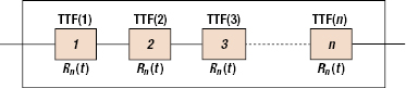
- A group of components that are essential for the performance of the system and/or its mission are drawn in series (Figure 17.1).
- Components that can substitute for other components are drawn in parallel (Figure 17.3).
- Each block in the diagram is like a switch: it is closed when the component it represents is working and is opened when the component has failed. Any closed path through the diagram is a success path.
The failure behavior of all the redundant components must be specified. Some of the common types of redundancies are:
- Active Redundancy or Hot Standby. The component has the same failure rate as if it was operating in the system.
- Passive Redundancy, Spare, or Cold Standby. The standby component cannot fail. This is generally assumed for spare or shelf items.
- Warm Standby. The standby component has a lower hazard rate than the operating component. This is usually a realistic assumption.
This chapter describes how to design, analyze, and evaluate the reliability of a system based on the parts, assemblies, and subsystems that compose a system. Most of the concepts in this chapter are explained using one level of the system hierarchical process. For example, we will illustrate how to compute system reliability if we know the reliabilities of the subsystems. Then the same methods and logic can be used to combine assemblies of the subsystem, and so on.
17.2 Series System
In a series system, all subsystems must operate successfully if the system is to function or operate successfully. This implies that the failure of any subsystem will cause the entire system to fail.
The reliability block diagram of a series system is shown in Figure 17.1. The reliability of each block is represented by Ri(t) and the times to failure are represented by TTF(i). The units need not be physically connected in series for the system to be called a series system.
System reliability can be determined using the basic principles of probability theory. We make the assumption that all the subsystems are probabilistically independent. This means that whether or not one subsystem works does not depend on the success or failure of other subsystems.
Let us first consider the static case. Let Ri be the reliability of the ith subsystem, i = 1, 2, … , n. Let Es be the event that the system functions successfully and Ei be the event that each subsystem i functions successfully (i = 1, 2, …, n). Then
because the system will function if and only if all the subsystems function. If all the events Ei, i = 1, 2, … , n, are probabilistically independent, then

Equation 17.2 can be generalized for time-dependent or dynamic reliability models. If we denote the time to failure random variable for the ith subsystem by Ti, i = 1, 2, … , n. Then for the series system, the system reliability is given by
If we assume that all the random variables, Ti, i = 1, 2, … , n, are independent, then
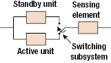
Hence, we can state the following equation:

From Equation 17.2, it is clear that the reliability of the system reduces with an increase in the number of subsystems or components in the series system (see Figure 17.2).

Assume that the time-to-failure distribution for each subsystem/component of a system is exponential and has a constant failure rate, λi. For the exponential distribution, the component reliability is
Hence, the system reliability is given by:

The system also has an exponential time-to-failure distribution, and the constant system failure rate is given by:

and the mean time between failures for the system is

The system hazard rate is constant if all the components of the system are in series and have constant hazard rates. The assumptions of a constant hazard rate and a series system make the mathematics simple, but this is rarely the case in practice.
For the general case, taking the log of both sides of Equation 17.5, we have

Also recall that

which means that
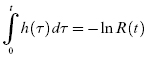
or
Applying this to Equation 17.10, we have
Thus, the hazard rate for the system is the sum of the hazard rates of the subsystems under the assumption that the time-to-failure random variables for all the subsystems are independent, regardless of the form of the pdf's for the time-to-failure random variables for all the subsystems.
17.3 Products with Redundancy
Redundancy exists when one or more of the parts of a system can fail and the system will still be able to function with the parts that remain operational. Two common types of redundancy are active and standby. In active redundancy, all the parts are energized and operational during the operation of a system. In active redundancy, the parts will consume life at the same rate as the individual components.
In standby redundancy, some parts do not contribute to the operation of the system, and they get switched on only when there are failures in the active parts. In standby redundancy, the parts in standby ideally should last longer than the parts in active redundancy.
There are three conceptual types of standby redundancy: cold, warm, and hot. In cold standby, the secondary parts are shut down until needed. This lowers the number of hours that the part is active and typically assumes negligible consumption of useful life, but the transient stresses on the parts during switching may be high. This transient stress can cause faster consumption of life during switching. In warm standby, the secondary parts are usually active, but are idling or unloaded. In hot standby, the secondary parts form an active parallel system. The life of the hot standby parts are assumed to be consumed at the same rate as active parts.
17.3.1 Active Redundancy
An active redundant system is a standard “parallel” system. That fails only when all components have failed. Sometimes, the parallel system is called a 1-out-of-n or (1, n) system, which implies that only one (or more) out of n subsystems has to operate for the system to be operational or functional. Thus, a series system is an n-out-of-n system. The reliability block diagram of a parallel system is given in Figure 17.3.
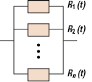
The units need not be physically connected in parallel for the system to be called a parallel system. The system will fail if all of the subsystems or all of the components fail by time t, or the system will survive the mission time, t, if at least one of the units survives by time t. Then, the system reliability can be expressed as
where Qs(t) is the probability of system failure, or

under the assumption that the time to failure random variables for all the subsystems are probabilistically independent.
The system reliability for a mission time, t, is
For the static situation or for an implied fixed value of t, we have an equation similar to Equation 17.2, which is given by

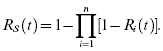
Figure 17.4 shows the effect of component reliability on system reliability for an active parallel system for a static situation.
We can use Equation 17.2 and Equation 17.18 to calculate the reliability of systems that have subsystems in series and in parallel. This is illustrated in Example 17.3.
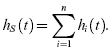
After we know the system reliability function from Equation 17.17, the system hazard rate is given by:
where fS(t) is the system time-to-failure probability density function (pdf). The mean life, or the expected life, of the system is determined by:

where TS is the time to failure for the system.
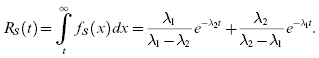
For example, if the system consists of two units (n = 2) with an exponential failure distribution with constant failure rates λ1 and λ2, then the system mean life is given by Equation 17.21. Note that the system mean life is not equal to the reciprocal of the sum of the component's constant failure rates, and we can prove that the hazard rate is not constant over time, although the individual unit failure rates are constant.
If the time to failure for all n components is exponentially distributed with MTBF θ, then the MTBF for the system is given by

Here, θ = MTBF for every component or subsystem. Thus, each additional component increases the expected life of the system but at a slower and slower rate. This motivates us to consider standby redundant systems in the next section.
17.3.2 Standby Systems
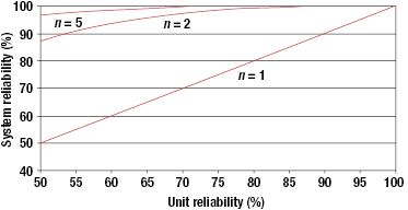
A standby system consists of an active unit or subsystem and one or more inactive (standby) units that become active in the event of the failure of the functioning unit. The failures of active units are signaled by a sensing subsystem, and the standby unit is brought to action by a switching subsystem. The simplest standby configuration is a two-unit system, as shown in Figure 17.6. In general, there will be n number of units with (n − 1) of them in standby.
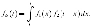
Let us now develop the system reliability models for the standby situation with two subsystems. Let fi(t) be the pdf for the time to failure random variable, Ti, for the ith unit, i = 1, 2, and fS(t) be the pdf for the time to failure random variable, TS, for the system. Let us first consider a situation with only two units under the assumption that the sensing and the switching mechanisms are perfect. Thus, the second unit is switched on when the first component fails. Thus, TS = T1 + T2, and TS is nothing but a convolution of two random variables. Hence,
Similarly, if we have a primary active component and two standby components, we have

We can evaluate Equation 17.23 when both T1 and T2 have the exponential distribution as below:

From Equation 17.25, we have
The MTBFS, θS, for the system is given by
as is expected since TS = T1 + T2 and E[TS] = E[T1] + E[T2].
When the active and the standby units have equal constant failure rates, λ, and the switching and sensing units are perfect, the reliability function for such a system is given by
We can rewrite Equation 17.26 in the form
or as shown in Equation 17.30, where AR(2) is the contribution to the reliability value of the system by the second component
This can easily be generalized to a situation where we have one primary component and two or more standby components. For example, if we have one primary component and (n − 1) standby components, and all have exponential time to failure with a constant failure rate of λ, then the system reliability function is given by

17.3.3 Standby Systems with Imperfect Switching
Switching and sensing systems are not perfect. There are many ways these systems can fail. Let us look at a situation where the switching and sensing unit simply fails to operate when called upon to do its job. Let the probability that the switch works when required be pSW. Then, the system reliability for one primary component and one standby is given by

When the main and the standby units have exponential time-to-failure distributions, we can use Equation 17.30 to develop the following equation:
Now, let us generalize Equation 17.32, where the switching and sensing unit is dynamic and the switching and sensing unit starts its life at the same time the active or the main unit starts its life. Let TSW denote the time to failure for the switching and sensing unit, where its pdf and reliability functions are denoted by fSW(t) and RSW(t), respectively. Then the reliability of the system is given by

If the time to failure of the switching and sensing unit follows an exponential distribution with a failure rate of λSW, then Equation 17.34 reduces to

If we consider a special case where both the main unit and the standby units have exponential time-to-failure distributions with parameter λ, then Equation 17.35 reduces to
17.3.4 Shared Load Parallel Models
A situation that is common in engineering systems and their design is called a shared load parallel model. In this case, the two parallel components/units share a load together. Thus, the load on each unit is half of the total load. When one of the units fails, the other unit must take the full load. An example of a shared load parallel configuration is one in which two bolts are used to hold a machine element, and if one of the bolts fails, the other bolt must take the full load. The stresses on the bolt now will be doubled, and this will result in an increased hazard rate for the surviving bolt.
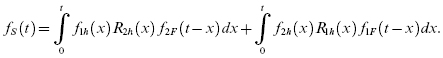
Let f1h(t) and f2h(t) be pdfs for the time to failure for the two units under half or shared load, and f1F(t) and f2F(t) be the pdfs under the full load for each unit, respectively. In this case, we can prove that the pdf for the time to failure of the system is
The reliability function for the system if both units are identical (such as identical bolts), where we have f1h(t) = f2h(t) = fh(t) and f1F(t) = f2F(t) = fF(t), can be shown as

If both fh(t) and fF(t) follow exponential distributions with parameters λh and λF, respectively, then it can be shown that the reliability function for the system is
17.3.5 (k, n) Systems
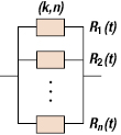
A system consisting of n components is called a k-out-of-n or (k, n) system if the system only operates when at least k or more components are in an operating state. The reliability block diagram (Figure 17.8) for the k-out-of-n system is drawn similar to the parallel system, but in this case at least k items need to be operating for the system to be functional.
In this configuration, the system works if and only if at least k components out of the n components work, 1 ≤ k ≤ n. When Ri = R(t) for all i, with the assumption that the time to failure random variables are independent, we have
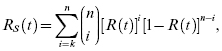
and the probability of system failure, where Q(t) = 1 − R(t), is

The probability density function can be determined by
and the system hazard rate is given by
If R(t) = e−t/θ, for an exponential case, the MTBF for the system is given by
The reliability function for the system is mathematically complex to compute in a closed form when the components have different failure distributions. We will present the methodology later on in this chapter to solve this problem.
17.3.6 Limits of Redundancy
It is often difficult to realize the benefits of redundancy if there are common mode failures, load sharing, and switching and standby failures. Common mode failures are caused by phenomena that create dependencies between two or more redundant parts and which then cause them to fail “simultaneously.” Common mode failures can be caused by many things, such as common electric connections, shared environmental stresses, and common maintenance problems.
Load sharing failures occur when the failure of one part increases the stress level of other parts. This increased stress level can affect the life of the active parts. For redundant engines, motors, pumps, structures, and many other systems and devices in active parallel setup, the failure of one part may increase the load on the other parts and decrease their times to failure (or increase their hazard rates).
Several common assumptions are made regarding the switching and sensing of a standby system. Regarding switching, it is often assumed that switching is in one direction only, that switching devices respond only when directed to switch by the monitor, and that switching devices do not fail if not energized. Regarding standby, the general assumption is that standby nonoperating units cannot fail if not energized. When any of these idealizations are not met, switching and standby failures occur. Monitor or sensing failures include both dynamic (failure to switch when active path fails) and static (switching when not required) failures.
17.4 Complex System Reliability
If the system architecture cannot be decomposed into some combination of series-parallel structures, it is deemed a complex system. There are three methods for reliability analysis of a complex system using Figure 17.9 as an example.

17.4.1 Complete Enumeration Method
The complete enumeration method is based on a list of all possible combinations of states of the subsystems. Table 17.1 lists 25 = 32 system states, which are all the possible states of the system given in Figure 17.9 based on the states of the subsystems. The symbol O stands for “system in operating state,” and F stands for “system in failed state.” Letters in uppercase denote a unit in an operating state, and lowercase letters denote a unit in a failed state.
Table 17.1 Complete enumeration example
| System description | System condition | System status |
|---|---|---|
| All components operable | ABCDE | O |
| One unit in failed state | aBCDE | O |
| AbCDE | O | |
| ABcDE | O | |
| ABCdE | O | |
| ABCDe | O | |
| Two units in failed state | abCDE | F |
| aBcDE | O | |
| aBCdE | O | |
| aBCDe | O | |
| AbcDE | F | |
| AbCdE | O | |
| AbCDe | O | |
| ABcdE | O | |
| ABcDe | O | |
| ABCde | O | |
| Three units in failed state | ABcde | F |
| AbCde | O | |
| AbcDe | F | |
| AbcdE | F | |
| aBCde | O | |
| aBcDe | O | |
| aBcdE | O | |
| abCDe | F | |
| abCdE | F | |
| abcDE | F | |
| Four units in failed state | Abcde | F |
| aBcde | F | |
| abCde | F | |
| abcDe | F | |
| abcdE | F | |
| All five units in failed state | abcde | F |
Each combination representing the system status can be written as a product of the probabilities of units being in a given state; for example, the second combination in Table 17.1 can be written as (1 − RA)RBRCRDRE, where (1 − RA) denotes the probability of failure of unit A by time t. The system reliability can be written as the sum of all the combinations for which the system is in operating state, O, that is,
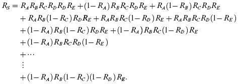
After simplification, the system reliability can be represented as
17.4.2 Conditional Probability Method
The conditional probability method is based on the law of total probability, which allows system decomposition by a selected unit and its state at time t. For example, system reliability is equal to the reliability of the system given that unit A is in its operating state at time t, denoted by RS|AS, times the reliability of unit A, plus the reliability of the system, given that unit A is in a failed state at time t, RS|AF, times the unreliability of unit A, or
This decomposition process continues until each term is written in terms of the reliability and unreliability of each of the units.
As an example, consider the system given in Figure 17.9 and decompose the system using unit C. Then, the system reliability can be written as
If the unit C is in the operating state at time t, the system reduces to the configuration shown in Figure 17.10. Therefore, the system reliability, given that unit C is in its operating state at time t, is equal to the series-parallel combination as shown above, or


If unit C is in a failed state at time t, the system reduces to the configuration given in Figure 17.11. Then the system reliability, given that unit C is in a failed state, is given by
The system reliability is obtained by substituting Equation 17.49 and Equation 17.50 into Equation 17.48:
The system reliability is expressed in terms of the reliabilities of its components. Simplification of Equation 17.51 gives the same expression as Equation 17.46.
17.4.3 Concept of Coherent Structures
In general, the concept of coherent systems can be used to determine the reliability of any system (Barlow and Proschan 1975; Leemis 1995; Rausand and Hoyland 2003). The performance of each of the n components in the system is represented by a binary indicator variable, xi, which takes the value 1 if the ith component functions and 0 if the ith component fails. Similarly, the binary variable ϕ indicates the state of the system, and ϕ is a function of x = (x1, … , xn).
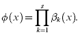
The function ϕ(x) is called the structure function of the system. The structure function is represented by using the concept of minimal paths and minimal cuts. A minimal path is the minimal set of components whose functioning ensures the functioning of the system. A minimal cut is the minimal set of components whose failures would cause the system to fail. Let αj(x) be the jth minimal path series structure for path Aj, j = 1, … , p, and βk(x) be the kth minimal parallel cut structure for cut Bk, k = 1, … , s. Then we have
and
The structure function of the system using minimum cuts is given by Equation 17.54, and the structure function using minimum cuts is given by Equation 17.55, as follows:

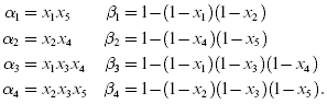
Let us consider the following bridge structure given in Figure 17.12. For the bridge structure (Figure 17.12), we have four minimal paths and four minimal cuts, and their structure functions are given below:

Then the reliability of the system is given by
where X is the random vector of the states of the components (X1, … , Xn).
We can develop the structure function by putting structure functions of minimum paths and minimum cuts in Equation 17.54 and Equation 17.55, respectively. When we do the expansion, we should remember that each xi is a binary variable that takes values of 0 or 1, and hence, ![]() for any positive integer n is also a binary variable and takes the value of 0 or 1. If we do the expansion using Equation 17.54 or Equation 17.55, we can prove that the structure function for the system in Figure 17.12 is
for any positive integer n is also a binary variable and takes the value of 0 or 1. If we do the expansion using Equation 17.54 or Equation 17.55, we can prove that the structure function for the system in Figure 17.12 is
If Ri is the reliability of the ith component, then we know that
and the system reliability for the bridge structure is given by
If all Ri = R = 0.9, we have
The exact calculations for RS are generally very tedious because the paths and the cuts are dependent, since they may contain the same component. Bounds on system reliability are given by

Using these bounds for the bridge structure, we have, when Ri = R = 0.9, the upper bound, RU, on system reliability, RS, is

and the lower bound, RL, is
The bounds on system reliability using the concepts of minimum paths and cuts can be improved.
17.5 Summary
The reliability of the system is a function of the reliabilities of its components and building blocks. To design, analyze, and evaluate the reliability and maintainability characteristics of a system, there must be an understanding of the system's relationships to all the subsystems, assemblies, and components. Many times this can be accomplished through logical and mathematical models. Engineering analysis of a system has to be conducted in order to develop a reliability model. Based on this analysis, a reliability block diagram is developed, which can be used to calculate various measures of reliability and maintainability. A reliability block diagram is a pictorial way of showing the success or failure combinations for a system. A system reliability block diagram presents a logical relationship of the system, subsystems, and components.
In a series system, all subsystems must operate successfully if the system is to function or operate successfully. This implies that the failure of any subsystem will cause the entire system to fail. Redundancy is a strategy to resolve this problem. Redundancy exists when one or more of the parts of a system can fail and the system will still be able to function with the parts that remain operational. Two common types of redundancy are active and standby. In active redundancy, all the parts are energized and operational during the operation of a system. In standby redundancy, some parts do not contribute to the operation of the system, and they get switched on only when there are failures in the active parts. In standby redundancy, the parts in standby ideally should last longer than the parts in active redundancy. It is often difficult to realize the benefits of redundancy if there are common mode failures, load sharing, and switching and standby failures. In addition to series systems, there are complex systems. If the system architecture cannot be decomposed into some combination of series-parallel structures, it is deemed a complex system. These two types of systems, series-parallel and complex, require different strategies for monitoring and evaluating system reliability.
Problems
17.1 The reliability block diagram of a system is given below. The number in each box is the reliability of the component. Find the reliability of the system.
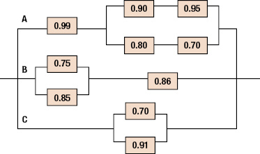
Thus, A, B, and C are three subsystems that are in parallel.
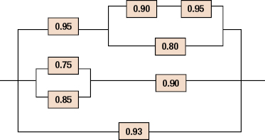
17.2 The reliability block diagram of a system is given below. The number in each box is the reliability of the component. Find the reliability of the system.
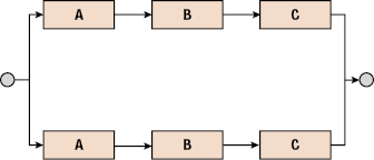
17.3 There are three components, A, B, and C, and they are represented by different blocks in the following two reliability block diagrams. Both reliability block diagrams use the same component twice. Let the reliabilities of the components be denoted by RA, RB, and RC.

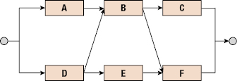
17.4 The reliability block diagram shown below is a complex system that cannot be decomposed into a “series-parallel” configuration. We want to determine the reliability equation for the system using the conditional probability method. We have decided to use the component B for the decomposition. Draw the two reliability block diagrams that result from “B operating” and “B failed” conditions.
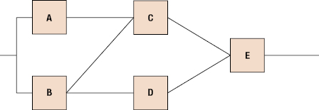
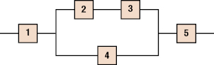
17.5 Consider the system shown in the block diagram and derive an equation for the reliability of the system. RX denotes the reliability of each component in the system, where X is the name of the component. For stage 3 (four C components in parallel), and it is a two-out-of-four system, that is, two components need to operate for the system to operate.

17.6 Derive (manually) the reliability equation of the system shown below. This is a complex dynamic system and the failure distribution for each component is shown in the table.
| Component | Failure Distribution | Parameter (in Hour or Equivalent) |
|---|---|---|
| A | Weibull 3 parameter | β = 3, η = 1000, γ = 100 |
| B | Exponential | MTBF = 1000 |
| C | Lognormal | Mean = 6, standard deviation = 0.5 |
| D | Weibull 3 parameter | β = 0.7, η = 150, γ = −100 |
| E | Normal | Mean = 250, standard deviation = 15 |
Find the following for this complex system:
What happens to the results if you switch the properties of component C and D?
17.7 Consider a series system composed of two subsystems where the first subsystem has a Weibull time to failure distribution with parameters η = 2 and θ = 200 hours. The second subsystem has an exponential time to failure distribution with θ = 300 hours. Develop the following functions for the system:
17.8 Consider a parallel system composed of two identical subsystems where the subsystem failure rate is λ, a constant.
17.9 A system consists of a basic unit and two standby units. All units (basic and the two standby) have an exponential distribution for time to failure with a failure rate of λ = 0.02 failures per hour. The probability that the switch will perform when required is 0.98.
17.10 Consider a two-unit pure parallel arrangement where each subsystem has a constant failure rate of λ, and compare this to a standby redundant arrangement that has a constant switch failure rate of λSW. Specifically, what is the maximum permissible value of λSW such that the pure parallel arrangement is superior to the standby arrangement?
17.11 Consider a system that has seven components and the system will work if any five of the seven components work (5-out-of-7 system). Each component has a reliability of 0.92 for a given period. Find the reliability of the system.
17.12 Consider the following system, which consists of five components. The reliabilities of the components are as follows:
17.13 A system has four components with the following reliability block diagram:

The reliability of the four components is as follows: