
3
Probability and Life Distributions for Reliability Analysis
In reliability engineering, data are often collected from analysis of incoming parts and materials, tests during and after manufacturing, fielded products, and warranty returns. If the collected data can be modeled, then properties of the model can be used to make decisions for product design, manufacture, reliability assessment, and logistics support (e.g., maintainability and operational availability).
In this chapter, discrete and continuous probability models (distributions) are introduced, along with their key properties. Two discrete distributions (binomial and Poisson) and five continuous distributions (exponential, normal, lognormal, Weibull, and gamma) that are commonly used in reliability modeling and hazard rate assessments are presented.
3.1 Discrete Distributions
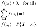
A discrete random variable is a random variable with a finite (or countably infinite) set of values. If a discrete random variable (X) has a set of discrete possible values (x1, x2, … xn), a probability mass function (pmf), f(xi) , is a function such that
The cumulative distribution function (cdf) is written as:
The mean, μ, and variance, σ2, of a discrete random variable are defined using the pmf as (see also Chapter 2):
3.1.1 Binomial Distribution
The binomial distribution is a discrete probability distribution applicable in situations where there are only two mutually exclusive outcomes for each trial or test. For example, for a roll of a die, the probability is one to six that a specified number will occur (success) and five to six that it will not occur (failure). This example, known as a “Bernoulli trial,” is a random experiment with only two possible outcomes, denoted as “success” or “failure.” Of course, success or failure is defined by the experiment. In some experiments, the probability of the result not being a certain number may be defined as a success.
The pmf, f(x), for the binomial distribution gives the probability of exactly k successes in m attempts:
where p is the probability of the defined success, q (or 1 – p) is the probability of failure, m is the number of independent trials, k is the number of successes in m trials, and the combinational formula is defined by
where ! is the symbol for factorial. Since (p + q) equals 1, raising both sides to a power j gives
The general equation is

The binomial expansion of the term on the left in Equation 3.7 gives the probabilities of j or less number of successes in j trials, as represented by the binomial distribution. For example, for three components or trials each with equal probability of success (p) or failure (q), Equation 3.7 becomes:
The four terms in the expansion of (p + q)3 give the values of the probabilities for getting 3, 2, 1, and no successes, respectively. That is, for m = 3 and the probability of success = p, f(3) = p3, f(2) = 3p2q, f(1) = 3pq2, and f(0) = q3.
The binomial expansion is also useful when there are products with different success and failure probabilities. The formula for the binomial expansion in this case is
where i pertains to the ith component in a system consisting of m components. For example, for a system of three different components, the expansion takes the form
where the first term on the right side of the equation gives the probability of success of all three components, the second term (in parentheses) gives the probability of success of any two components, the third term (in parentheses) gives the probability of success of any one component, and the last term gives the probability of failure for all components.
The cdf for the binomial distribution, F(k), gives the probability of k or fewer successes in m trials. It is defined by using the pmf for the binomial distribution,

For a binomial distribution, the mean, μ is given by
and the variance is given by
3.1.2 Poisson Distribution
In situations where the probability of success (p) is very low and the number (m) of samples tested (i.e., the number of Bernoulli trials conducted) is large, it is cumbersome to evaluate the binomial coefficients. A Poisson distribution is useful in such cases.
The pmf of the Poisson distribution is given as:
where μ is the mean and also the variance of the Poisson random variable.
For a Poisson distribution for m Bernoulli trials, with the probability of success in each trial equal to p, the mean and the variance are given by:
The Poisson distribution is widely used in industrial and quality engineering applications. It is also the foundation of some of the attribute control charts. For example, it is used in applications such as determination of particles of contamination in a manufacturing environment, number of power outages, and flaws in rolls of polymers.
3.1.3 Other Discrete Distributions
Other discrete distributions that are used in reliability analysis include the geometric distribution, the negative binomial distribution, and the hypergeometric distribution.
With the geometric distribution, the Bernoulli trials are conducted until the first success is obtained. The geometric distribution has the “lack of memory” property, implying that the count of the number of trials can be started at any trial without affecting the underlying distribution. In this regard, this distribution is similar to the continuous exponential distribution, which will be described later.
With the negative binomial distribution (a generalization of the geometric distribution), the Bernoulli trials are conducted until a certain number of successes are obtained. Negative binomial distribution is, however, conceptually different from the binomial distribution, since the number of successes is predetermined, and the number of trials is a random variable.
With the hypergeometric distribution, testing or sampling is conducted without replacement from a population that has a certain number of defective products. The hypergeometric distribution differs from the binomial distribution in that the population is finite and the sampling from the population is made without replacement.
3.2 Continuous Distributions
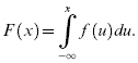
If the range of a random variable, X, extends over an interval (either finite or infinite) of real numbers, then X is a continuous random variable. The cdf is given by:
The probability density function (pdf) is analogous to pmf for discrete variables, and is denoted by f(x) , where f(x) is given by (if F(x) is differentiable):
which yields
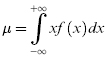
The mean, μ, and variance, σ2, of a continuous random variable are defined over the interval from –∞ to +∞ in terms of the probability density function as (see Chapter 2):

Reliability is concerned with the time to failure random variable T and thus X is replaced by T. Thus, Equation 3.19 corresponds to Equation 2.5 and Equation 3.20 corresponds to Equation 2.46.
3.2.1 Weibull Distribution
The Weibull distribution is a continuous distribution developed in 1939 by Waloddi Weibull (1939), and who presented it in detail in 1951 (Weibull 1951). The Weibull distribution is widely used for reliability analyses because a wide diversity of hazard rate curves can be modeled with it. The distribution can also be approximated to other distributions under special or limiting conditions. The Weibull distribution has been applied to life distributions for many engineered products, and has also been used for reliability testing, material strength, and warranty analysis.
The probability density function for a three-parameter Weibull probability distribution function is
where β > 0 is the shape parameter, η > 0 is the scale parameter, which is also denoted by θ in many references and books, and γ is the location or time delay parameter. The reliability function is given by

It can be shown that Equation 3.23 gives, for a duration t = γ + η, starting at time t = 0, a reliability value of R(t) = 36.8%, regardless of the value of β. Thus, for any Weibull failure probability density function, 36.8% of the products survive for t = γ + η.
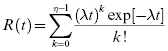
The time to failure of a product with a specified reliability, R, is given by
The hazard rate function for the Weibull distribution is given by

The conditional reliability function is (see Eq. 2.39):

Equation 3.26 gives the reliability for a new mission of duration t for which t1 hours of operation were previously accumulated up to the beginning of this new mission. It is seen that the Weibull distribution is generally dependent on both the age at the beginning of the mission and the mission duration (unless β = 1). In fact, this is true for most distributions, except for the exponential distribution (discussed later).
Table 3.1 lists the key parameters for a Weibull distribution and values for mean, median, mode, and standard deviation. The function Γ is the gamma function, for which the values are available from statistical tables and also are provided in Appendix B.
Table 3.1 Weibull distribution parameters
| Location | γ | |
| Shape parameter | β | |
| Scale parameter | η | |
| Mean (arithmetic average) | γ + η + Γ(1/β + 1) | |
| Median (B50, or time at 50% failure) | γ + η(ln2)1/β | |
| Mode (highest value of f(t)) | for β > 1 | γ + η(l − 1/β)1/β |
| for β = 1 | γ | |
| Standard deviation | ||
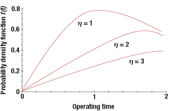
The shape parameter of a Weibull distribution determines the shape of the hazard rate function. With 0 < β < 1, the hazard rate decreases as a function of time, and can represent early life failures (i.e., infant mortality). A β = 1 indicates that the hazard rate is constant and is representative of the “useful life” period in the “idealized” bathtub curve (see Figure 2.6). A β > 1 indicates that the hazard rate is increasing and can represent wearout. Figure 3.2 shows the effects of β on the probability density function curve with η = 1 and γ = 0. Figure 3.3 shows the effect of β on the hazard rate curve with η = 1 and γ = 0.
The scale parameter η has the effect of scaling the time axis. Thus, for a fixed γ and β, an increase in η will stretch the distribution to the right while maintaining its starting location and shape (although there will be a decrease in the amplitude, since the total area under the probability density function curve must be equal to unity). Figure 3.4 shows the effect of η on the probability density function for β = 2 and γ = 0.


The location parameter locates the distribution along the time axis and thus estimates the earliest time to failure. For γ = 0, the distribution starts at t = 0. With γ > 0, this implies that the product has a failure-free operating period equal to γ. Figure 3.5 shows the effects of γ on the probability density function curve for β = 2 and η = 1. Note that if γ is positive, the distribution starts to the right of the t = 0 line, or the origin. If γ is negative, the distribution starts to the left of the origin, and could imply that failures had occurred prior to the time t = 0, such as during transportation or storage. Thus, there is a probability mass F(0) at t = 0, and the rest of the distribution for t > 0 is given in Figure 3.5. The Weibull distribution can also be formulated as a two-parameter distribution with γ = 0.
The reliability function for the two-parameter Weibull distribution is

and the hazard rate function is

The two-parameter Weibull distribution can be used to model skewed data. When β < 1, the failure rate for the Weibull distribution is decreasing and hence can be used to model infant mortality or a debugging period, situations when the reliability in terms of failure rate is improving, or reliability growth. When β = 1, the Weibull distribution is the same as the exponential distribution. When β > 1, the failure rate is increasing, and hence can model wearout and the end of useful life. Some examples of this are corrosion life, fatigue life, or the life of antifriction bearings, transmission gears, and electronic tubes.
The three-parameter Weibull distribution is a model when there is a minimum life or when the odds of the component failing before the minimum life are close to zero. Many strength characteristics of systems do have a minimum value significantly greater than zero. Some examples are electrical resistance, capacitance, and fatigue strength.

3.2.2 Exponential Distribution
The exponential distribution is a single-parameter distribution that can be viewed as a special case of a Weibull distribution, where β = 1. The probability density function has the form
where λ0 is a positive real number, often called the constant failure rate. The parameter λ0 is typically an unknown that must be calculated or estimated based on statistical methods discussed later in this section. Figure 3.6 gives a graph for an exponential distribution, with λ0 = 0.10. Table 3.2 summarizes the key parameters for the exponential distribution.

Once λ0 is known, the reliability can be determined from the probability density function as
The cdf or unreliability is given by
As mentioned, the hazard rate for the exponential distribution is constant:
The conditional reliability is
Equation 3.33 shows that previous usage (e.g., tests or missions) do not affect future reliability. This “as good as new” result stems from the fact that the hazard rate is a constant and the probability of a product failing is independent of the past history or use of the product.
The mean time to failure (MTTF) for an exponential distribution, also denoted by θ, is determined from the general equation for the mean of a continuous distribution:

Table 3.2 Exponential distribution parameter
| Scale parameter | 1/λ0 |
| Median (B50) | 0.693/λ0 |
| Mode (highest value of f(t)) | 0 |
| Standard deviation | 1/λ0 |
| Mean | 1/λ0 |
Thus, the MTTF or the MTBF is inversely proportional to the constant failure rate, and thus the reliability can be expressed as
The MTBF is sometimes misunderstood to be the life of the product or the time by which 50% of products will fail. For a mission time of t = MTBF, the reliability calculated from Equation 3.30 gives R(MTBF) = 0.368. Thus, only 36.8% of the products survive a mission time equal to the MTBF.
3.2.3 Estimation of Reliability for Exponential Distribution
For reliability tests in which the hazard rate is assumed to be constant, and the time to failure can be assumed to follow an exponential distribution, the constant failure rate can be estimated by life testing. There are various ways to test the items. Figure 3.7 gives an example of a failure-truncated test, in which n items on individual test stands are monitored to failure. The test ends as soon as there are r failures (without replacement r ≤ n), as shown in Figure 3.7.

 .
.The total time on test, TT, considering both failed and unfailed (or suspended) units, is calculated by the following equation:

Another test situation is called time-truncated testing. In Figure 3.8, there are n test stands (or n items on test in a test chamber). The units are monitored and replaced as soon as they fail. Testing for these units continues until some predetermined time, t0. In this case, the total time on test is

 , Failures.
Then the point estimator (minimum variance unbiased estimator) for θ, the MTBF, is
Further details are given in Chapter 13. Also, the point estimator for λ is
Chapter 13 will present the methodology for the point estimation and confidence interval for several test situations and underlying life distributions.
3.2.4 The Normal (Gaussian) Distribution
The normal distribution occurs whenever a random variable is affected by a sum of random effects, such that no single factor dominates. This motivation is based on central limit theorem, which states that under mild conditions, the sum of a large number of random variables is approximately normally distributed. It has been used to represent dimensional variability in manufactured goods, material properties, and measurement errors. It has also been used to assess product reliability.
The normal distribution has been used to model various physical, mechanical, electrical, or chemical properties of systems. Some examples are gas molecule velocity, wear, noise, the chamber pressure from firing ammunition, the tensile strength of aluminum alloy steel, the capacity variation of electrical condensers, electrical power consumption in a given area, generator output voltage, and electrical resistance.
The probability density function for the normal distribution is based on the following Gaussian function:
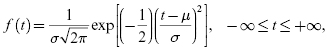
where the parameter μ is the mean or the MTTF, and σ is the standard deviation of the distribution. The parameters for a normal distribution are listed in Table 3.3. Figure 3.9 shows the shape of the probability density function for the normal distribution.
Table 3.3 Normal distribution parameters
| Mean (arithmetic average) | μ |
| Median (B50 or 50th percentile) | μ |
| Mode (highest value of f(t)) | μ |
| Location parameter | μ |
| Shape parameter/standard deviation | σ |
| s (an estimate of σ) | B50 − B16 |

The cdf, or unreliability, for the normal distribution is:

A normal random variable with mean equal to zero and variance of 1 is called a standard normal variable (Z), and its pdf is given by
where z ≡ (t – μ)/σ.
The properties of the standard normal variable, in particular the cumulative probability distribution function, are tabulated in statistical tables (provided in Appendix C). Table 3.4 provides the percentage values of the areas under the normal curve at different distances from the mean in terms of multiples of σ. For example,
and
Table 3.4 Areas under the normal curve
| μ – 1σ = 15.87% | μ + 1σ = 84.130% |
| μ – 2σ = 2.28% | μ + 2σ = 97.720% |
| μ – 3σ = 0.135% | μ + 3σ = 99.865% |
| μ – 4σ = 0.003% | μ + 4σ = 99.997% |
There is no closed-form solution to the integral of Equation 3.41, and, therefore, the values for the area under the normal distribution curve are obtained from the standard normal tables by converting the random variable, t, to a random variable, z, using the transformation:
given by Equation 3.42. We have
or
and
where ϕ(.) is the pdf for the standard normal distribution and Φ(z) is the cdf for the standard normal random variable Z.
From Equation 3.48, we can prove that the normal distribution has an increasing hazard rate (IHR). The normal distribution has been used to describe the failure distribution for products that show wearout and that degrade with time. The life of tire tread and the cutting edges of machine tools fit this description. In these situations, life is given by a mean value of μ, and the variability about the mean value is defined through standard deviation. When the normal distribution is used, the probabilities of a failure occurring before or after this mean time are equal because the mean is the same as the median.
3.2.5 The Lognormal Distribution
For a continuous random variable, there may be a situation in which the random variable is a product of a series of random variables. The lognormal distribution is a positively skewed distribution and has been used to model situations where large occurrences are concentrated at the tail (left) end of the range. Some examples are the amount of electricity used by different customers, the downtime of systems, the time to repair, the light intensities of light bulbs, the concentration of chemical process residues, and automotive mileage accumulation by different customers. For example, the wear on a system may be proportional to the product of the magnitudes of the loads acting on it. Thus, a random variable may be modeled as a lognormal random variable if it can be thought of as the multiplicative product of many independent random variables each of which is positive. If a random variable has lognormal distribution, then the logarithm of the random variable is normally distributed. If X is a random variable with a normal distribution, then Y = eX has a lognormal distribution; or if Y has lognormal distribution, then X = log Y has normal distribution.
Suppose Y is the product of n independent random variables given by
Taking the natural logarithm of Equation 3.49 gives
Then ln Y may have approximately normal distribution based on the central limit theorem.
The lognormal distribution has been shown to apply to many engineering situations, such as the strengths of metals and the dimensions of structural elements, and to biological parameters, such as loads on bone joints. Lognormal distributions have been applied in reliability engineering to describe failures caused by fatigue and to model time to repair for maintainability analysis. The probability density function for the lognormal distribution is:

where σ is the standard deviation of the logarithms of all times to failure, and μ is the mean of the logarithms of all times to failure. If random variable T follows a lognormal distribution with parameters μ and σ, then ln T follows a normal distribution so that
The cdf (unreliability) for the lognormal distribution is:
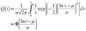
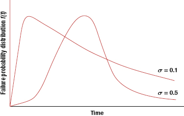
The probability density function for two values of σ are as shown in Figure 3.10. The key parameters for the lognormal distribution are provided in Table 3.5.
The MTTF for a population for which the time to failure follows a lognormal distribution is given by
and the failure rate is given by
The hazard rate for the lognormal distribution is neither always increasing nor always decreasing. It takes different shapes, depending on the parameters μ and σ. We can prove that the hazard rate of a lognormal distribution is increasing on average (called IHRA).
From the basic properties of the logarithm operator, it can be shown that if variables X and Y are distributed lognormally, then the product random variable Z = XY is also lognormally distributed.
Table 3.5 Lognormal distribution parameters
| Mean | exp[μ + 0.5σ2] |
| Variance | |
| Median (B50 or time at 50% failures) | B50 = eμ |
| Mode (highest value of f(t)) | t = exp[μ – σ2] |
| Location parameter | eμ |
| Shape parameter | σ |
| s (estimate of σ) | ln(B50/B16) |
3.2.6 Gamma Distribution
The probability density function for the gamma distribution is given by
where Γ(η) is the gamma function (values for this function are given in Appendix B). The gamma distribution has two parameters, η and λ, where η is called the shape parameter and λ is called the scale parameter. The gamma distribution reduces to the exponential distribution if η = 1. Adding η exponential distributions, η ≥ 1, with the same parameter λ, provides the gamma distribution. Thus, the gamma distribution can be used to model time to the ηth failure of a system if the underlying system/component failure distribution is exponential with parameter λ. We can also state that if Ti is exponentially distributed with parameter λ, i = 1, 2, … , η, then T = T1 + T2 + … + Tη has a gamma distribution with parameters λ and η. This distribution could be used if we wanted to determine the system reliability for redundancy with identical components all having a constant failure rate.
From Equation 3.56, the cumulative distribution or the unreliability function is

If η is an integer, then the gamma distribution is also called the Erlang distribution, and it can be shown by successive integration by parts that

Then,
and
Also,
and
The failure rate for the gamma distribution is decreasing when η < 1, is constant when η = 1(because it is an exponential distribution), and is increasing when η > 1.
3.3 Probability Plots
Probability plotting is a method for determining whether data (observations) conform to a hypothesized distribution. Typically, computer software is used to assess the hypothesized distribution and determine the parameters of the underlying distribution. The method used by the software tools is analogous to using constructed probability plotting paper to plot data. The time-to-failure data is ordered from the smallest to the largest in value in an appropriate metric (e.g., time to failure and cycles to failure). An estimate of the percent of unreliability is selected. The data are plotted against a theoretical distribution in such a way that the points should form a straight line if the data come from the hypothesized distribution. The data are plotted on probability plotting papers (these are distribution specific), with ordered times to failure in the x-axis and the estimate of percent unreliability as the y-axis. A best-fit straight line is drawn through the plotted data points.
The time to failure data used for the x-axis is obtained from the field or testing. The estimate of unreliability against which to plot this time-to-failure data is not that obvious. Several different techniques, such as “midpoint plotting position,” “expected plotting position,” “median plotting position,” “median rank,” and Kaplan–Meier ranks (in software) are used for this estimate. Table 3.6 provides estimates for unreliability based on different estimation schemes for a sample size of 20.
The median rank value for the ith failure, Qi, is given by the solution to the following equation:
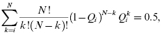
where N is the sample size, i is the failure number, and Qi is the median rank (or estimate of unreliability at the failure time of the ith failure). Equation 3.64, which estimates the median plotting positions, can be used in place of the median rank as an approximation:
Table 3.6 Examples of cdf estimates for N = 20

The axes used for the plots are not linear. The axes are different for each probability distribution and are created by linearizing the cmf or unreliability function, typically by taking the logarithm of both sides repeatedly. For example, mathematical manipulation based on Equation 3.27 for a two-parameter Weibull distribution will result in an ordinate (y-axis) as log log reciprocal of R(t) = 1 – Q(t) scale and the abscissa as a log scale of time to failure, and is derived below:
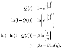
where x = ln(t) and y = ln(−ln(1 − Q(t))).
Once the probability plots are prepared for different distributions, the goodness of fit of the plots is one factor in determining which distribution is the right fit for the data. Probability distributions for data analysis should be selected based on their ability to fit the data and for physics-based reasons. There should be a physics-based argument for selection of a distribution that draws from the failure model for the mechanism(s) that caused the failures. These decisions are not always clear-cut. For example, the lognormal and the Weibull distribution both model fatigue failure data well, and hence it is often possible for both to fit the failure data; thus, experience-based engineering judgments need to be made.
There is no reason to assume that all the time-to-failure data taken together need to fit only one failure distribution. Since the failures in a product can be caused by more than one mechanism, it is possible that some of the failures are caused by one mechanism and the others by a different mechanism. In that case, no single probability distribution will fit the data well. Even if it appears that one distribution fits all the data, that distribution may not have good predictive ability. That is why it may be necessary to separate the failures by mechanisms into sets and then fit separate distributions for each set.
Table 3.7 shows times to failure separated into two groups by failure mechanism. Figure 3.11 shows the Weibull probability plots for the competing failure mechanism data. Note that the shape and scale factors for the two sets are distinct, with one set having a decreasing hazard rate (β = 0.67) and the other set having an increasing hazard rate (β = 4.33). If the data are plotted together, the result shows an almost constant hazard rate. However, spare part and support decisions made based on results from a combined data analysis can be misleading and counterproductive.
Table 3.7 Time to failure data separated by failure mechanism

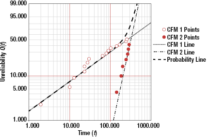
When the life data contains two or more life segments—such as infant mortality, useful life, and wearout—a mixed Weibull distribution can be used to fit parts of the data with different distribution parameters. A curved or S-shaped Weibull probability plot (in either two or three parameters) is an indication that a mixed Weibull distribution may be present.
Statistical analysis provides no magical way of projecting into the future. The results from an analysis are only as good as the assumed model and assumptions, including how failure is defined, the validity of the data, how the model is used, and taking into consideration the tail of the distribution and the limits of extrapolations and interpolations. The following example demonstrates the absurdity of extrapolating times to failure beyond their reasonable limits.
3.4 Summary
The reliability function is used to describe the probability of successful system operation during a system's life. A natural question is then, “What is the shape of a reliability function for a particular system?” There are basically three ways in which this can be determined:
- Test many systems to failure using a mission profile identical to use conditions. This would provide an empirical curve based on the histogram that can give some idea about the nature of the underlying life distribution.
- Test many subsystems and components to failure under use conditions recreated in the test environment. This empirically provides the component reliability functions. Then derive analytically or numerically or through simulation the system reliability function. (Chapter 17 covers topics related to system reliability.)
- Based on past experience with similar systems, hypothesize the underlying failure distribution. Fewer systems can be tested to determine the parameters needed to adapt the failure distribution to a particular situation. However, this will not account for new failure mechanisms or new use conditions.
In some cases, the failure physics involved in a particular situation may lead to the hypothesis of a particular distribution. For example, fatigue of certain metals tends to follow either a lognormal or Weibull distribution. Once a distribution is selected, the parameters for a particular application can be ascertained using statistical or graphical procedures.
In this chapter, various distributions were presented. However, the most appropriate distribution(s) for a particular failure mechanism or product that exhibits certain failure mechanisms must be determined by the actual data, and not guessed. The distribution(s) that best fit the data and that also make sense in terms of the failure processes should be used.
Problems
3.1 Prove that for a binomial distribution in which the number of trials is m and the probability of success in each trial is p, the mean and the variance are equal to mp and mp(1 – p), respectively.
3.2 Prove that for a Poisson distribution, the mean and the variance are equal to the Poisson parameter μ.
3.3 Compare the results of Examples 3.2 and 3.5. What is the reason for the differences?
3.4 Consider a system that has seven components; the system will work if any five of the seven components work. Each component has a reliability of 0.930 for a given period. Find the reliability of the system.
3.5 For an exponential distribution, show that the time to 50% failure is given by 0.693/λ0.
3.6 For an exponential distribution, show that the standard deviation is equal to 1/λ0.
3.7 Show that for a two-parameter Weibull distribution, for t = η, the reliability R(t) = 0.368, irrespective of β.
3.8 The front wheel roller bearing life for a car is modeled by a two-parameter Weibull distribution with the following two parameters: β = 3.7, θ = 145,000 mi. What is the 100,000-mi reliability for a bearing?
3.9 The life distribution (life in years of continuous use) of hard disk drives for a computer system follows the Weibull distribution with the following parameters:
3.10 The life distribution for miles to failure for the engine of a Lexus car follows the Weibull distribution with
If a certain model has 200,000 engines in the field with a life of 100,000 mi, how many engines on average will fail in the next 100 mi of use out of the 200,000 engines?
3.11 A component has the normal distribution for time to failure, with μ = 26,000 hours and σ = 3500 hours.
3.12 The time to failure random variable for a battery follows a normal distribution, with μ = 800 hours and σ = 65 hours.
- 700 hours
- 710 hours.
3.13 The time to failure for the hard disk drives for a computer system follows a normal distribution with
3.14 The time to repair a communication network system follows a lognormal distribution with μ = 3.50 and σ = 0.75. The time is in minutes.
3.15 The time to repair a copy machine follows the lognormal distribution with μ = 2.70 and σ = 0.65. Time is in minutes.
3.16 The time to failure for a copy machine follows a gamma distribution with parameters η = 2 and λ = 0.004.
3.17 Describe two examples of systems that require a failure-free operating period, without any maintenance. What are the timeframes involved?
3.18 Describe two examples of systems that require a failure-free operating period, but may allow a maintenance period. Discuss the timeframes.
3.19 Show that the mode of the three parameter Weibull distribution is for
for β > 1.
3.20 A company knows that approximately 3 out of every 1000 processors that it manufactures are defective. What is the probability that out of the next 20 processors selected (at random):