Chapter 3. Routing Dynamically
Objectives
Upon completion of this chapter, you will be able to answer the following questions:
![]() What is the purpose of dynamic routing protocols?
What is the purpose of dynamic routing protocols?
![]() How does dynamic routing compare with static routing?
How does dynamic routing compare with static routing?
![]() How do dynamic routing protocols share route information and achieve convergence?
How do dynamic routing protocols share route information and achieve convergence?
![]() What are the differences between the categories of dynamic routing protocols?
What are the differences between the categories of dynamic routing protocols?
![]() How does the algorithm used by distance vector routing protocols determine the best path?
How does the algorithm used by distance vector routing protocols determine the best path?
![]() What are the different types of distance vector routing protocols?
What are the different types of distance vector routing protocols?
![]() How do you configure the RIP routing protocol?
How do you configure the RIP routing protocol?
![]() How do you configure the RIPng routing protocol?
How do you configure the RIPng routing protocol?
![]() How does the algorithm used by link-state routing protocols determine the best path?
How does the algorithm used by link-state routing protocols determine the best path?
![]() How do link-state routing protocols use information sent in link-state updates?
How do link-state routing protocols use information sent in link-state updates?
![]() What are the advantages and disadvantages of using link-state routing protocols?
What are the advantages and disadvantages of using link-state routing protocols?
![]() How do you determine the source route, administrative distance, and metric for a given route?
How do you determine the source route, administrative distance, and metric for a given route?
![]() How do you explain the concept of a parent/child relationship in a dynamically built routing table?
How do you explain the concept of a parent/child relationship in a dynamically built routing table?
![]() How do you describe the differences between the IPv4 route lookup process and the IPv6 route lookup process?
How do you describe the differences between the IPv4 route lookup process and the IPv6 route lookup process?
![]() Can you determine which route will be used to forward a packet upon analyzing a routing table?
Can you determine which route will be used to forward a packet upon analyzing a routing table?
Key Terms
This chapter uses the following key terms. You can find the definitions in the Glossary.
Routing Information Protocol (RIP)
Advanced Research Projects Agency Network (ARPANET)
Open Shortest Path First (OSPF)
Intermediate System-to-Intermediate System (IS-IS)
Interior Gateway Routing Protocol (IGRP)
Interior Gateway Protocols (IGP)
Exterior Gateway Protocols (EGP)
distance vector routing protocols
variable-length subnet mask (VLSM)
Introduction (3.0.1.1)
The data networks that we use in our everyday lives to learn, play, and work range from small, local networks to large, global internetworks. At home, a user may have a router and two or more computers. At work, an organization may have multiple routers and switches servicing the data communication needs of hundreds or even thousands of PCs.
Routers forward packets by using information in the routing table. Routes to remote networks can be learned by the router in two ways: static routes and dynamic routes.
In a large network with numerous networks and subnets, configuring and maintaining static routes between these networks requires a great deal of administrative and operational overhead. This operational overhead is especially cumbersome when changes to the network occur, such as a down link or implementing a new subnet. Implementing dynamic routing protocols can ease the burden of configuration and maintenance tasks and give the network scalability.
This chapter introduces dynamic routing protocols. It explores the benefits of using dynamic routing protocols, how different routing protocols are classified, and the metrics routing protocols use to determine the best path for network traffic. Other topics covered in this chapter include the characteristics of dynamic routing protocols and how the various routing protocols differ. Network professionals must understand the different routing protocols available in order to make informed decisions about when to use static or dynamic routing. They also need to know which dynamic routing protocol is most appropriate in a particular network environment.
![]() Class Activity 3.0.1.2: How Much Does This Cost?
Class Activity 3.0.1.2: How Much Does This Cost?
This modeling activity illustrates the network concept of routing cost.
You will be a member of a team of five students who travel routes to complete the activity scenarios. One digital camera or bring your own device (BYOD) with camera, a stopwatch, and the student file for this activity will be required per group. One person will function as the photographer and event recorder, as selected by each group. The remaining four team members will actively participate in the following scenarios.
A school or university classroom, hallway, outdoor track area, school parking lot, or any other location can serve as the venue for these activities.
Activity 1
The tallest person in the group establishes a start and finish line by marking 15 steps from start to finish, indicating the distance of the team route. Each student will take 15 steps from the start line toward the finish line and then stop on the 15th step—no further steps are allowed.
Note
Not all of the students may reach the same distance from the start line due to their height and stride differences. The photographer will take a group picture of the entire team’s final location after taking the 15 steps required.
Activity 2
A new start and finish line will be established; however, this time, a longer distance for the route will be established than the distance specified in Activity 1. No maximum steps are to be used as a basis for creating this particular route. One at a time, students will walk the new route from beginning to end twice.
Each team member will count the steps taken to complete the route. The recorder will time each student and, at the end of each team member’s route, record the time that it took to complete the full route and how many steps were taken, as recounted by each team member and recorded on the team’s student file.
After both activities have been completed, teams will use the digital picture taken for Activity 1 and their recorded data from Activity 2 file to answer the reflection questions.
Group answers can be discussed as a class, time permitting.
Dynamic Routing Protocols (3.1)
Dynamic routing protocols play an important role in today’s networks. The following sections describe several important benefits that dynamic routing protocols provide. In many networks, dynamic routing protocols are typically used with static routes.
The Evolution of Dynamic Routing Protocols (3.1.1.1)
Dynamic routing protocols have been used in networks since the late 1980s. One of the first routing protocols was Routing Information Protocol (RIP). RIP version 1 (RIPv1) was released in 1988, but some of the basic algorithms within the protocol were used on the Advanced Research Projects Agency Network (ARPANET) as early as 1969.
As networks evolved and became more complex, new routing protocols emerged. The RIP routing protocol was updated to accommodate growth in the network environment, into RIPv2. However, the newer version of RIP still does not scale to the larger network implementations of today. To address the needs of larger networks, two advanced routing protocols were developed: Open Shortest Path First (OSPF) and Intermediate System-to-Intermediate System (IS-IS). Cisco developed the Interior Gateway Routing Protocol (IGRP) and Enhanced IGRP (EIGRP), which also scales well in larger network implementations.
Additionally, there was the need to connect different internetworks and provide routing between them. The Border Gateway Protocol (BGP) is now used between Internet service providers (ISPs). BGP is also used between ISPs and their larger private clients to exchange routing information.
Table 3-1 classifies the protocols.

With the advent of numerous consumer devices using IP, the IPv4 addressing space is nearly exhausted; thus, IPv6 has emerged. To support the communication based on IPv6, newer versions of the IP routing protocols have been developed, as shown by the IPv6 row in Table 3-1.
RIP is the simplest of dynamic routing protocols and is used in this section to provide a basic level of routing protocol understanding.
Purpose of Dynamic Routing Protocols (3.1.1.2)
Routing protocols are used to facilitate the exchange of routing information between routers. A routing protocol is a set of processes, algorithms, and messages that are used to exchange routing information and populate the routing table with the routing protocol’s choice of best paths. The purpose of dynamic routing protocols includes:
![]() Discovery of remote networks
Discovery of remote networks
![]() Maintaining up-to-date routing information
Maintaining up-to-date routing information
![]() Choosing the best path to destination networks
Choosing the best path to destination networks
![]() Ability to find a new best path if the current path is no longer available
Ability to find a new best path if the current path is no longer available
The main components of dynamic routing protocols include:
![]() Data structures: Routing protocols typically use tables or databases for their operations. This information is kept in RAM.
Data structures: Routing protocols typically use tables or databases for their operations. This information is kept in RAM.
![]() Routing protocol messages: Routing protocols use various types of messages to discover neighboring routers, exchange routing information, and perform other tasks to learn and maintain accurate information about the network.
Routing protocol messages: Routing protocols use various types of messages to discover neighboring routers, exchange routing information, and perform other tasks to learn and maintain accurate information about the network.
![]() Algorithm: An algorithm is a finite list of steps used to accomplish a task. Routing protocols use algorithms for facilitating routing information and for best path determination.
Algorithm: An algorithm is a finite list of steps used to accomplish a task. Routing protocols use algorithms for facilitating routing information and for best path determination.
Figure 3-1 highlights the data structures, routing protocol messages, and routing algorithm used by EIGRP.

The Role of Dynamic Routing Protocols (3.1.1.3)
Routing protocols allow routers to dynamically share information about remote networks and automatically add this information to their own routing tables.
![]() Video 3.1.1.3: Routers Dynamically Share Updates
Video 3.1.1.3: Routers Dynamically Share Updates
Go to the online course and play the animation of three routers sharing updates dynamically.
Routing protocols determine the best path, or route, to each network. That route is then added to the routing table. A primary benefit of dynamic routing protocols is that routers exchange routing information when there is a topology change. This exchange allows routers to automatically learn about new networks and also to find alternate paths when there is a link failure to a current network.
Compared to static routing, dynamic routing protocols require less administrative overhead. However, the expense of using dynamic routing protocols is dedicating part of a router’s resources for protocol operation, including CPU time and network link bandwidth. Despite the benefits of dynamic routing, static routing still has its place. There are times when static routing is more appropriate and other times when dynamic routing is the better choice. Networks with moderate levels of complexity may have both static and dynamic routing configured.
![]() Activity 3.1.1.4: Identify Components of a Routing Protocol (EIGRP)
Activity 3.1.1.4: Identify Components of a Routing Protocol (EIGRP)
Go to the online course to perform these three practice activities.
Dynamic versus Static Routing (3.1.2)
Routing tables can contain directly connected, manually configured static routes and routes learned dynamically using a routing protocol. Network professionals must understand when to use static or dynamic routing. This section compares static routing and dynamic routing.
Using Static Routing (3.1.2.1)
Before identifying the benefits of dynamic routing protocols, consider the reasons why network professionals use static routing. Dynamic routing certainly has several advantages over static routing; however, static routing is still used in networks today. In fact, networks typically use a combination of both static and dynamic routing.
Static routing has several primary uses, including:
![]() Providing ease of routing table maintenance in smaller networks that are not expected to grow significantly.
Providing ease of routing table maintenance in smaller networks that are not expected to grow significantly.
![]() Routing to and from a stub network, which is a network with only one default route out and no knowledge of any remote networks.
Routing to and from a stub network, which is a network with only one default route out and no knowledge of any remote networks.
![]() Accessing a single default route (which is used to represent a path to any network that does not have a more specific match with another route in the routing table).
Accessing a single default route (which is used to represent a path to any network that does not have a more specific match with another route in the routing table).
Figure 3-2 provides a sample static routing scenario.

Static Routing Scorecard (3.1.2.2)
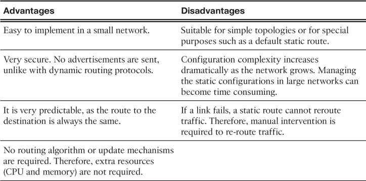
Static routing is easy to implement in a small network. Static routes stay the same, which makes them fairly easy to troubleshoot. Static routes do not send update messages and, therefore, require very little overhead.
The disadvantages of static routing include:
![]() They are not easy to implement in a large network.
They are not easy to implement in a large network.
![]() Managing the static configurations can become time consuming.
Managing the static configurations can become time consuming.
![]() If a link fails, a static route cannot reroute traffic.
If a link fails, a static route cannot reroute traffic.
Table 3-2 highlights the advantages and disadvantages of static routing.
Using Dynamic Routing Protocols (3.1.2.3)
Dynamic routing protocols help the network administrator manage the time-consuming and exacting process of configuring and maintaining static routes.
Imagine maintaining the static routing configurations for the seven routers in Figure 3-3.

What if the company grew and now has four regions and 28 routers to manage, as shown in Figure 3-4? What happens when a link goes down? How do you ensure that redundant paths are available?

Dynamic routing is the best choice for large networks like the one shown in Figure 3-4.
Dynamic Routing Scorecard (3.1.2.4)
Dynamic routing protocols work well in any type of network consisting of several routers. They are scalable and automatically determine better routes if there is a change in the topology. Although there is more to the configuration of dynamic routing protocols, they are simpler to configure in a large network.
There are disadvantages to dynamic routing. Dynamic routing requires knowledge of additional commands. It is also less secure than static routing because the interfaces identified by the routing protocol send routing updates out. Routes taken may differ between packets. The routing algorithm uses additional CPU, RAM, and link bandwidth.
Table 3-3 highlights the advantages and disadvantages of dynamic routing.

Notice how dynamic routing addresses the disadvantages of static routing.
![]() Activity 3.1.2.5: Compare Static and Dynamic Routing
Activity 3.1.2.5: Compare Static and Dynamic Routing
Go to the online course to perform this practice activity.
Routing Protocol Operating Fundamentals (3.1.3)
All routing protocols basically perform the same tasks. They all exchange routing updates and converge to build routing tables that are used by the router to make packet forwarding decisions. This section provides an overview of routing protocol fundamentals.
Dynamic Routing Protocol Operation (3.1.3.1)
All routing protocols are designed to learn about remote networks and to quickly adapt whenever there is a change in the topology. The method that a routing protocol uses to accomplish this depends upon the algorithm it uses and the operational characteristics of that protocol.
In general, the operations of a dynamic routing protocol can be described as follows:
1. The router sends and receives routing messages on its interfaces.
2. The router shares routing messages and routing information with other routers that are using the same routing protocol.
3. Routers exchange routing information to learn about remote networks.
4. When a router detects a topology change, the routing protocol can advertise this change to other routers.
![]() Video 3.1.3.1: Routing Protocol Operation
Video 3.1.3.1: Routing Protocol Operation
Go to the online course and play the animation of two routers sharing routing updates.
Cold Start (3.1.3.2)
All routing protocols follow the same patterns of operation. When a router powers up, it knows nothing about the network topology. It does not even know that there are devices on the other end of its links. The only information that a router has is from its own saved configuration file stored in NVRAM.
After a router boots successfully, it applies the saved configuration. If the IP addressing is configured correctly, then the router initially discovers its own directly connected networks.
![]() Video 3.1.3.2: Directly Connected Networks Detected
Video 3.1.3.2: Directly Connected Networks Detected
Go to the online course to view an animation of the initial discovery of connected networks for each router.
Notice how the routers proceed through the boot process and then discover any directly connected networks and subnet masks. This information is added to their routing tables as follows:
![]() R1 adds the 10.1.0.0 network available through interface FastEthernet 0/0 and adds 10.2.0.0 available through interface Serial 0/0/0.
R1 adds the 10.1.0.0 network available through interface FastEthernet 0/0 and adds 10.2.0.0 available through interface Serial 0/0/0.
![]() R2 adds the 10.2.0.0 network available through interface Serial 0/0/0 and adds 10.3.0.0 available through interface Serial 0/0/1.
R2 adds the 10.2.0.0 network available through interface Serial 0/0/0 and adds 10.3.0.0 available through interface Serial 0/0/1.
![]() R3 adds the 10.3.0.0 network available through interface Serial 0/0/1 and adds 10.4.0.0 available through interface FastEthernet 0/0.
R3 adds the 10.3.0.0 network available through interface Serial 0/0/1 and adds 10.4.0.0 available through interface FastEthernet 0/0.
With this initial information, the routers then proceed to find additional route sources for their routing tables.
Network Discovery (3.1.3.3)
After initial boot up and discovery, the routing table is updated with all directly connected networks and the interfaces those networks reside on.
If a routing protocol is configured, the next step is for the router to begin exchanging routing updates to learn about any remote routes.
The router sends an update packet out all interfaces that are enabled on the router. The update contains the information in the routing table, which currently comprises all directly connected networks.
At the same time, the router also receives and processes similar updates from other connected routers. Upon receiving an update, the router checks it for new network information. Any networks that are not currently listed in the routing table are added.
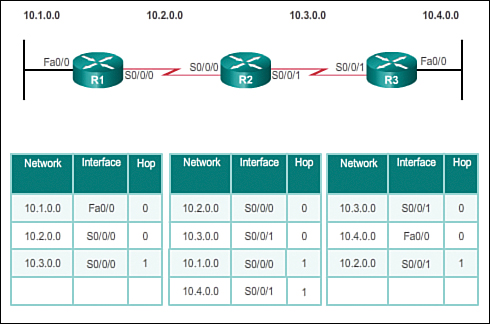
Figure 3-5 depicts an example topology setup between three routers, R1, R2, and R3. Notice that only the directly connected networks are listed in each router’s respective routing table.

Based on this topology, a listing of the different updates that R1, R2, and R3 send and receive during initial convergence is provided:
![]() Sends an update about network 10.1.0.0 out the Serial 0/0/0 interface
Sends an update about network 10.1.0.0 out the Serial 0/0/0 interface
![]() Sends an update about network 10.2.0.0 out the FastEthernet 0/0 interface
Sends an update about network 10.2.0.0 out the FastEthernet 0/0 interface
![]() Receives update from R2 about network 10.3.0.0 and increments the hop count by 1
Receives update from R2 about network 10.3.0.0 and increments the hop count by 1
![]() Stores network 10.3.0.0 in the routing table via Serial 0/0/0 with a metric of 1
Stores network 10.3.0.0 in the routing table via Serial 0/0/0 with a metric of 1
R2:
![]() Sends an update about network 10.3.0.0 out the Serial 0/0/0 interface
Sends an update about network 10.3.0.0 out the Serial 0/0/0 interface
![]() Sends an update about network 10.2.0.0 out the Serial 0/0/1 interface
Sends an update about network 10.2.0.0 out the Serial 0/0/1 interface
![]() Receives an update from R1 about network 10.1.0.0 and increments the hop count by 1
Receives an update from R1 about network 10.1.0.0 and increments the hop count by 1
![]() Stores network 10.1.0.0 in the routing table via Serial 0/0/0 with a metric of 1
Stores network 10.1.0.0 in the routing table via Serial 0/0/0 with a metric of 1
![]() Receives an update from R3 about network 10.4.0.0 and increments the hop count by 1
Receives an update from R3 about network 10.4.0.0 and increments the hop count by 1
![]() Stores network 10.4.0.0 in the routing table via Serial 0/0/1 with a metric of 1
Stores network 10.4.0.0 in the routing table via Serial 0/0/1 with a metric of 1
R3:
![]() Sends an update about network 10.4.0.0 out the Serial 0/0/1 interface
Sends an update about network 10.4.0.0 out the Serial 0/0/1 interface
![]() Sends an update about network 10.3.0.0 out the FastEthernet 0/0 interface
Sends an update about network 10.3.0.0 out the FastEthernet 0/0 interface
![]() Receives an update from R2 about network 10.2.0.0 and increments the hop count by 1
Receives an update from R2 about network 10.2.0.0 and increments the hop count by 1
![]() Stores network 10.2.0.0 in the routing table via Serial 0/0/1 with a metric of 1
Stores network 10.2.0.0 in the routing table via Serial 0/0/1 with a metric of 1
Figure 3-6 displays the routing tables after the initial exchange.
![]() Video 3.1.3.3: Initial Exchange
Video 3.1.3.3: Initial Exchange
Go to the online course and play the animation of R1, R2, and R3 starting the initial exchange.
After this first round of update exchanges, each router knows about the connected networks of its directly connected neighbors. However, did you notice that R1 does not yet know about 10.4.0.0 and that R3 does not yet know about 10.1.0.0? Full knowledge and a converged network do not take place until there is another exchange of routing information.
Exchanging the Routing Information (3.1.3.4)
At this point the routers have knowledge about their own directly connected networks and about the connected networks of their immediate neighbors. Continuing the journey toward convergence, the routers exchange the next round of periodic updates. Each router again checks the updates for new information.
After initial discovery is complete, each router continues the convergence process by sending and receiving the following updates.
R1:
![]() Sends an update about network 10.1.0.0 out the Serial 0/0/0 interface
Sends an update about network 10.1.0.0 out the Serial 0/0/0 interface
![]() Sends an update about networks 10.2.0.0 and 10.3.0.0 out the FastEthernet 0/0 interface
Sends an update about networks 10.2.0.0 and 10.3.0.0 out the FastEthernet 0/0 interface
![]() Receives an update from R2 about network 10.4.0.0 and increments the hop count by 1
Receives an update from R2 about network 10.4.0.0 and increments the hop count by 1
![]() Stores network 10.4.0.0 in the routing table via Serial 0/0/0 with a metric of 2
Stores network 10.4.0.0 in the routing table via Serial 0/0/0 with a metric of 2
![]() Same update from R2 contains information about network 10.3.0.0 with a metric of 1. There is no change; therefore, the routing information remains the same.
Same update from R2 contains information about network 10.3.0.0 with a metric of 1. There is no change; therefore, the routing information remains the same.
R2:
![]() Sends an update about networks 10.3.0.0 and 10.4.0.0 out of Serial 0/0/0 interface
Sends an update about networks 10.3.0.0 and 10.4.0.0 out of Serial 0/0/0 interface
![]() Sends an update about networks 10.1.0.0 and 10.2.0.0 out of Serial 0/0/1 interface
Sends an update about networks 10.1.0.0 and 10.2.0.0 out of Serial 0/0/1 interface
![]() Receives an update from R1 about network 10.1.0.0. There is no change; therefore, the routing information remains the same.
Receives an update from R1 about network 10.1.0.0. There is no change; therefore, the routing information remains the same.
![]() Receives an update from R3 about network 10.4.0.0. There is no change; therefore, the routing information remains the same.
Receives an update from R3 about network 10.4.0.0. There is no change; therefore, the routing information remains the same.
![]() Sends an update about network 10.4.0.0 out the Serial 0/0/1 interface
Sends an update about network 10.4.0.0 out the Serial 0/0/1 interface
![]() Sends an update about networks 10.2.0.0 and 10.3.0.0 out the FastEthernet 0/0 interface
Sends an update about networks 10.2.0.0 and 10.3.0.0 out the FastEthernet 0/0 interface
![]() Receives an update from R2 about network 10.1.0.0 and increments the hop count by 1
Receives an update from R2 about network 10.1.0.0 and increments the hop count by 1
![]() Stores network 10.1.0.0 in the routing table via Serial 0/0/1 with a metric of 2
Stores network 10.1.0.0 in the routing table via Serial 0/0/1 with a metric of 2
![]() Same update from R2 contains information about network 10.2.0.0 with a metric of 1. There is no change; therefore, the routing information remains the same.
Same update from R2 contains information about network 10.2.0.0 with a metric of 1. There is no change; therefore, the routing information remains the same.
Figure 3-7 displays the routing tables after the routers have converged.

Go to the online course and play an animation of R1, R2, and R3 sending the latest routing table to their neighbors.
Distance vector routing protocols typically implement a routing loop prevention technique known as split horizon. Split horizon prevents information from being sent out the same interface from which it was received. For example, R2 does not send an update containing the network 10.1.0.0 out of Serial 0/0/0, because R2 learned about network 10.1.0.0 through Serial 0/0/0.
After routers within a network have converged, the router can then use the information within the route table to determine the best path to reach a destination. Different routing protocols have different ways of calculating the best path.
Achieving Convergence (3.1.3.5)
The network has converged when all routers have complete and accurate information about the entire network, as shown in Figure 3-7. Convergence is the time it takes routers to share information, calculate best paths, and update their routing tables. A network is not completely operable until the network has converged; therefore, most networks require short convergence times.
Convergence is both collaborative and independent. The routers share information with each other, but must independently calculate the impacts of the topology change on their own routes. Because they develop an agreement with the new topology independently, they are said to converge on this consensus.
Convergence properties include the speed of propagation of routing information and the calculation of optimal paths. The speed of propagation refers to the amount of time it takes for routers within the network to forward routing information.
As shown in Figure 3-8, routing protocols can be rated based on the speed to convergence; the faster the convergence, the better the routing protocol. Generally, older protocols, such as RIP, are slow to converge, whereas modern protocols, such as EIGRP and OSPF, converge more quickly.

![]() Packet Tracer Activity 3.1.3.6: Investigating Convergence
Packet Tracer Activity 3.1.3.6: Investigating Convergence
This activity will help you identify important information in routing tables and witness the process of network convergence.
Types of Routing Protocols (3.1.4)
Table 3-1 showed how routing protocols can be classified according to various characteristics. This section gives an overview of the most common IP routing protocols. Most of these routing protocols will be examined in detail in other chapters. For now, this section gives a very brief overview of each protocol.
Classifying Routing Protocols (3.1.4.1)
Routing protocols can be classified into different groups according to their characteristics. Specifically, routing protocols can be classified by their:
![]() Purpose: Interior Gateway Protocol (IGP) or Exterior Gateway Protocol (EGP)
Purpose: Interior Gateway Protocol (IGP) or Exterior Gateway Protocol (EGP)
![]() Operation: Distance vector protocol, link-state protocol, or path-vector protocol
Operation: Distance vector protocol, link-state protocol, or path-vector protocol
![]() Behavior: Classful (legacy) or classless protocol
Behavior: Classful (legacy) or classless protocol
For example, IPv4 routing protocols are classified as follows:
![]() RIPv1 (legacy): IGP, distance vector, classful protocol
RIPv1 (legacy): IGP, distance vector, classful protocol
![]() IGRP (legacy): IGP, distance vector, classful protocol developed by Cisco (deprecated from 12.2 IOS and later)
IGRP (legacy): IGP, distance vector, classful protocol developed by Cisco (deprecated from 12.2 IOS and later)
![]() RIPv2: IGP, distance vector, classless protocol
RIPv2: IGP, distance vector, classless protocol
![]() EIGRP: IGP, distance vector, classless protocol developed by Cisco
EIGRP: IGP, distance vector, classless protocol developed by Cisco
![]() OSPF: IGP, link-state, classless protocol
OSPF: IGP, link-state, classless protocol
![]() IS-IS: IGP, link-state, classless protocol
IS-IS: IGP, link-state, classless protocol
![]() BGP: EGP, path-vector, classless protocol
BGP: EGP, path-vector, classless protocol
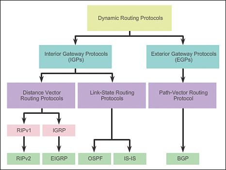
The classful routing protocols, RIPv1 and IGRP, are legacy protocols and are only used in older networks. These routing protocols have evolved into the classless routing protocols, RIPv2 and EIGRP, respectively. Link-state routing protocols are classless by nature.
Figure 3-9 displays a hierarchical view of dynamic routing protocol classification.
IGP and EGP Routing Protocols (3.1.4.2)
An autonomous system (AS) is a collection of routers under a common administration such as a company or an organization. An AS is also known as a routing domain. Typical examples of an AS are a company’s internal network and an ISP’s network.
The Internet is based on the AS concept; therefore, two types of routing protocols are required:
![]() Interior Gateway Protocols (IGP): Used for routing within an AS. It is also referred to as intra-AS routing. Companies, organizations, and even service providers use an IGP on their internal networks. IGPs include RIP, EIGRP, OSPF, and IS-IS.
Interior Gateway Protocols (IGP): Used for routing within an AS. It is also referred to as intra-AS routing. Companies, organizations, and even service providers use an IGP on their internal networks. IGPs include RIP, EIGRP, OSPF, and IS-IS.
![]() Exterior Gateway Protocols (EGP): Used for routing between autonomous systems. It is also referred to as inter-AS routing. Service providers and large companies may interconnect using an EGP. The Border Gateway Protocol (BGP) is the only currently viable EGP and is the official routing protocol used by the Internet.
Exterior Gateway Protocols (EGP): Used for routing between autonomous systems. It is also referred to as inter-AS routing. Service providers and large companies may interconnect using an EGP. The Border Gateway Protocol (BGP) is the only currently viable EGP and is the official routing protocol used by the Internet.
Note
Because BGP is the only EGP available, the term EGP is rarely used; instead, most engineers simply refer to BGP.
The example in Figure 3-10 provides simple scenarios highlighting the deployment of IGPs, BGP, and static routing.

There are five individual autonomous systems in the scenario:
![]() ISP-1: This is an AS and it uses IS-IS as the IGP. It interconnects with other autonomous systems and service providers using BGP to explicitly control how traffic is routed.
ISP-1: This is an AS and it uses IS-IS as the IGP. It interconnects with other autonomous systems and service providers using BGP to explicitly control how traffic is routed.
![]() ISP-2: This is an AS and it uses OSPF as the IGP. It interconnects with other autonomous systems and service providers using BGP to explicitly control how traffic is routed.
ISP-2: This is an AS and it uses OSPF as the IGP. It interconnects with other autonomous systems and service providers using BGP to explicitly control how traffic is routed.
![]() AS-1: This is a large organization and it uses EIGRP as the IGP. Because it is multihomed (i.e., connects to two different service providers), it uses BGP to explicitly control how traffic enters and leaves the AS.
AS-1: This is a large organization and it uses EIGRP as the IGP. Because it is multihomed (i.e., connects to two different service providers), it uses BGP to explicitly control how traffic enters and leaves the AS.
![]() AS-2: This is a medium-sized organization and it uses OSPF as the IGP. It is also multihomed; therefore, it uses BGP to explicitly control how traffic enters and leaves the AS.
AS-2: This is a medium-sized organization and it uses OSPF as the IGP. It is also multihomed; therefore, it uses BGP to explicitly control how traffic enters and leaves the AS.
![]() AS-3: This is a small organization with older routers within the AS; it uses RIP as the IGP. BGP is not required because it is single-homed (i.e., connects to one service provider). Instead, static routing is implemented between the AS and the service provider.
AS-3: This is a small organization with older routers within the AS; it uses RIP as the IGP. BGP is not required because it is single-homed (i.e., connects to one service provider). Instead, static routing is implemented between the AS and the service provider.
Note
BGP is beyond the scope of this course and is not discussed in detail.
Distance Vector Routing Protocols (3.1.4.3)
![]()
Distance Vector Routing Protocols
Distance vector means that routes are advertised by providing two characteristics:
![]() Distance: Identifies how far it is to the destination network and is based on a metric such as the hop count, cost, bandwidth, delay, and more
Distance: Identifies how far it is to the destination network and is based on a metric such as the hop count, cost, bandwidth, delay, and more
![]() Vector: Specifies the direction of the next-hop router or exit interface to reach the destination
Vector: Specifies the direction of the next-hop router or exit interface to reach the destination
For example, in Figure 3-11, R1 knows that the distance to reach network 172.16.3.0/24 is one hop and that the direction is out of the interface Serial 0/0/0 toward R2.

A router using a distance vector routing protocol does not have the knowledge of the entire path to a destination network. Distance vector protocols use routers as sign posts along the path to the final destination. The only information a router knows about a remote network is the distance or metric to reach that network and which path or interface to use to get there. Distance vector routing protocols do not have an actual map of the network topology.
There are four distance vector IPv4 IGPs:
![]() RIPv1: First generation legacy protocol
RIPv1: First generation legacy protocol
![]() RIPv2: Simple distance vector routing protocol
RIPv2: Simple distance vector routing protocol
![]() IGRP: First generation Cisco proprietary protocol (obsolete and replaced by EIGRP)
IGRP: First generation Cisco proprietary protocol (obsolete and replaced by EIGRP)
![]() EIGRP: Advanced version of distance vector routing
EIGRP: Advanced version of distance vector routing
Link-State Routing Protocols (3.1.4.4)
![]()
Link State Routing Protocols
In contrast to distance vector routing protocol operation, a router configured with a link-state routing protocol can create a complete view or topology of the network by gathering information from all of the other routers.
To continue our analogy of sign posts, using a link-state routing protocol is like having a complete map of the network topology. The sign posts along the way from source to destination are not necessary, because all link-state routers are using an identical map of the network. A link-state router uses the link-state information to create a topology map and to select the best path to all destination networks in the topology.
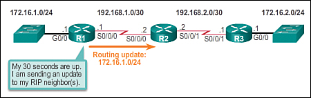
RIP-enabled routers send periodic updates of their routing information to their neighbors. Link-state routing protocols do not use periodic updates. After the network has converged, a link-state update is only sent when there is a change in the topology. For example, in Figure 3-12, the link-state update is sent when the 172.16.3.0 network goes down.

![]() Video 3.1.4.4: Link-State Protocol Operation
Video 3.1.4.4: Link-State Protocol Operation
Go to the online course and play the animation to see how a link-state update is only sent when the 172.16.3.0 network goes down.
Link-state protocols work best in situations where:
![]() The network design is hierarchical, usually occurring in large networks
The network design is hierarchical, usually occurring in large networks
![]() Fast convergence of the network is crucial
Fast convergence of the network is crucial
![]() The administrators have good knowledge of the implemented link-state routing protocol
The administrators have good knowledge of the implemented link-state routing protocol
There are two link-state IPv4 IGPs:
![]() OSPF: Popular standards-based routing protocol
OSPF: Popular standards-based routing protocol
![]() IS-IS: Popular in provider networks
IS-IS: Popular in provider networks
Classful Routing Protocols (3.1.4.5)
The biggest distinction between classful and classless routing protocols is that classful routing protocols do not send subnet mask information in their routing updates. Classless routing protocols include subnet mask information in the routing updates.
The two original IPv4 routing protocols developed were RIPv1 and IGRP. They were created when network addresses were allocated based on classes (i.e., class A, B, or C). At that time, a routing protocol did not need to include the subnet mask in the routing update, because the network mask could be determined based on the first octet of the network address.
Note
Only RIPv1 and IGRP are classful. All other IPv4 and IPv6 routing protocols are classless. Classful addressing has never been a part of IPv6.
The fact that RIPv1 and IGRP do not include subnet mask information in their updates means that they cannot provide variable-length subnet masks (VLSMs) and Classless Inter-Domain Routing (CIDR).
Classful routing protocols also create problems in discontiguous networks. A discontiguous network is when subnets from the same classful major network address are separated by a different classful network address.
To illustrate the shortcoming of classful routing, refer to the topology in Figure 3-13.

Notice that the LANs of R1 (172.16.1.0/24) and R3 (172.16.2.0/24) are both subnets of the same class B network (172.16.0.0/16). They are separated by different classful network addresses (192.168.1.0/30 and 192.168.2.0/30).
When R1 forwards an update to R2, RIPv1 does not include the subnet mask information with the update; it only forwards the class B network address 172.16.0.0.
R2 receives and processes the update. It then creates and adds an entry for the class B 172.16.0.0/16 network in the routing table, as shown in Figure 3-14.

When R3 forwards an update to R2, it also does not include the subnet mask information and therefore only forwards the classful network address 172.16.0.0.
R2 receives and processes the update and adds another entry for the classful network address 172.16.0.0/16 to its routing table, as shown in Figure 3-15. When there are two entries with identical metrics in the routing table, the router shares the load of the traffic equally among the two links. This is known as load balancing.
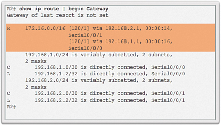
Discontiguous networks have a negative impact on a network. For example, a ping to 172.16.1.1 would return “U.U.U” because R2 would forward the first ping out its Serial 0/0/1 interface toward R3, and R3 would return a Destination Unreachable (U) error code to R2. The second ping would exit out of R2’s Serial 0/0/0 interface toward R1, and R1 would return a successful code (.). This pattern would continue until the ping command is done.
Classless Routing Protocols (3.1.4.6)
Modern networks no longer use classful IP addressing and the subnet mask cannot be determined by the value of the first octet. The classless IPv4 routing protocols (RIPv2, EIGRP, OSPF, and IS-IS) all include the subnet mask information with the network address in routing updates. Classless routing protocols support VLSM and CIDR.
IPv6 routing protocols are classless. The distinction whether a routing protocol is classful or classless typically only applies to IPv4 routing protocols. All IPv6 routing protocols are considered classless because they include the prefix-length with the IPv6 address.
Figures 3-16 through 3-18 illustrate how classless routing solves the issues created with classful routing.


In the discontiguous network design of Figure 3-16, the classless protocol RIPv2 has been implemented on all three routers. When R1 forwards an update to R2, RIPv2 includes the subnet mask information with the update 172.16.1.0/24.
In Figure 3-17, R2 receives, processes, and adds two entries in the routing table. The first line displays the classful network address 172.16.0.0 with the /24 subnet mask of the update. This is known as the parent route. The second entry displays the VLSM network address 172.16.1.0 with the exit and next-hop address. This is referred to as the child route. Parent routes never include an exit interface or next-hop IP address.
When R3 forwards an update to R2, RIPv2 includes the subnet mask information with the update 172.16.2.0/24.
R2 receives, processes, and adds another child route entry 172.16.2.0/24 under the parent route entry 172.16.0.0, as shown in Figure 3-18.
A ping from R2 to 172.16.1.1 would now be successful.
Routing Protocol Characteristics (3.1.4.7)
Routing protocols can be compared based on the following characteristics:
![]() Speed of convergence: Speed of convergence defines how quickly the routers in the network topology share routing information and reach a state of consistent knowledge. The faster the convergence, the more preferable the protocol. Routing loops can occur when inconsistent routing tables are not updated due to slow convergence in a changing network.
Speed of convergence: Speed of convergence defines how quickly the routers in the network topology share routing information and reach a state of consistent knowledge. The faster the convergence, the more preferable the protocol. Routing loops can occur when inconsistent routing tables are not updated due to slow convergence in a changing network.
![]() Scalability: Scalability defines how large a network can become, based on the routing protocol that is deployed. The larger the network is, the more scalable the routing protocol needs to be.
Scalability: Scalability defines how large a network can become, based on the routing protocol that is deployed. The larger the network is, the more scalable the routing protocol needs to be.
![]() Classful or classless (use of VLSM): Classful routing protocols do not include the subnet mask and cannot support variable-length subnet mask (VLSM). Classless routing protocols include the subnet mask in the updates. Classless routing protocols support VLSM and better route summarization.
Classful or classless (use of VLSM): Classful routing protocols do not include the subnet mask and cannot support variable-length subnet mask (VLSM). Classless routing protocols include the subnet mask in the updates. Classless routing protocols support VLSM and better route summarization.
![]() Resource usage: Resource usage includes the requirements of a routing protocol such as memory space (RAM), CPU utilization, and link bandwidth utilization. Higher resource requirements necessitate more powerful hardware to support the routing protocol operation, in addition to the packet forwarding processes.
Resource usage: Resource usage includes the requirements of a routing protocol such as memory space (RAM), CPU utilization, and link bandwidth utilization. Higher resource requirements necessitate more powerful hardware to support the routing protocol operation, in addition to the packet forwarding processes.
![]() Implementation and maintenance: Implementation and maintenance describes the level of knowledge that is required for a network administrator to implement and maintain the network based on the routing protocol deployed.
Implementation and maintenance: Implementation and maintenance describes the level of knowledge that is required for a network administrator to implement and maintain the network based on the routing protocol deployed.
Table 3-4 summarizes the characteristics of each routing protocol.

Routing Protocol Metrics (3.1.4.8)
There are cases when a routing protocol learns of more than one route to the same destination. To select the best path, the routing protocol must be able to evaluate and differentiate between the available paths. This is accomplished through the use of routing metrics.
A metric is a measurable value that is assigned by the routing protocol to different routes based on the usefulness of that route. In situations where there are multiple paths to the same remote network, the routing metrics are used to determine the overall “cost” of a path from source to destination. Routing protocols determine the best path based on the route with the lowest cost.
Different routing protocols use different metrics. The metric used by one routing protocol is not comparable to the metric used by another routing protocol. Two different routing protocols might choose different paths to the same destination.
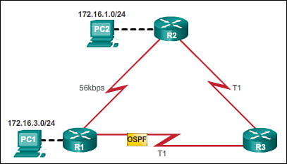
For example, assume that PC1 wants to send a packet to PC2. In Figure 3-19, the RIP routing protocol has been enabled on all routers and the network has converged. RIP makes a routing protocol decision based on the least number of hops. Therefore, when the packet arrives on R1, the best route to reach the PC2 network would be to send it directly to R2 even though the link is much slower that all other links.

In Figure 3-20, the OSPF routing protocol has been enabled on all routers and the network has converged. OSPF makes a routing protocol decision based on the best bandwidth. Therefore, when the packet arrives on R1, the best route to reach the PC2 network would be to send it to R3, which would then forward it to R2.
![]() Video 3.1.4.8: Routing Protocols and Their Metrics
Video 3.1.4.8: Routing Protocols and Their Metrics
Go to the online course and play the animation showing that RIP would choose the path with the least number of hops, whereas OSPF would choose the path with the highest bandwidth.
![]() Activity 3.1.4.9: Classify Dynamic Routing Protocols
Activity 3.1.4.9: Classify Dynamic Routing Protocols
Go to the online course to perform this practice activity.
![]() Activity 3.1.4.10: Compare Routing Protocols
Activity 3.1.4.10: Compare Routing Protocols
Go to the online course to perform this practice activity.
![]() Activity 3.1.4.11: Match the Metric to the Protocol
Activity 3.1.4.11: Match the Metric to the Protocol
Go to the online course to perform this practice activity.
Distance Vector Dynamic Routing (3.2)
This section describes the characteristics, operations, and functionality of distance vector routing protocols. Understanding the operation of distance vector routing is critical to enabling, verifying, and troubleshooting these protocols.
Distance Vector Technologies (3.2.1.1)
Distance vector routing protocols share updates between neighbors. Neighbors are routers that share a link and are configured to use the same routing protocol. The router is only aware of the network addresses of its own interfaces and the remote network addresses it can reach through its neighbors. Routers using distance vector routing are not aware of the network topology.
Some distance vector routing protocols send periodic updates. For example, RIP sends a periodic update to all of its neighbors every 30 seconds. RIP does this even if the topology has not changed; it continues to send updates. RIPv1 reaches all of its neighbors by sending updates to the all-hosts IPv4 address of 255.255.255.255, a broadcast.
The broadcasting of periodic updates is inefficient because the updates consume bandwidth and consume network device CPU resources. Every network device has to process a broadcast message. RIPv2 and EIGRP, instead, use multicast addresses so that only neighbors that need updates will receive them. EIGRP can also send a unicast message to only the affected neighbor. Additionally, EIGRP only sends an update when needed, instead of periodically.
As shown in Figure 3-21, the two modern IPv4 distance vector routing protocols are RIPv2 and EIGRP. RIPv1 and IGRP are listed only for historical accuracy.

Distance Vector Algorithm (3.2.1.2)
At the core of the distance vector protocol is the routing algorithm. The algorithm is used to calculate the best paths and then send that information to the neighbors.
The algorithm used for the routing protocols defines the following processes:
![]() Mechanism for sending and receiving routing information
Mechanism for sending and receiving routing information
![]() Mechanism for calculating the best paths and installing routes in the routing table
Mechanism for calculating the best paths and installing routes in the routing table
![]() Mechanism for detecting and reacting to topology changes
Mechanism for detecting and reacting to topology changes
![]() Video 3.2.1.2: Routers Route Packets
Video 3.2.1.2: Routers Route Packets
Go to the online course and play the animation to see how the RIP routing protocol adds and deletes routes from a routing table.
In the animation in the online course, R1 and R2 are configured with the RIP routing protocol. The algorithm sends and receives updates. Both R1 and R2 then glean new information from the update. In this case, each router learns about a new network. The algorithm on each router makes its calculations independently and updates the routing table with the new information. When the LAN on R2 goes down, the algorithm constructs a triggered update and sends it to R1. R1 then removes the network from the routing table.
Different routing protocols use different algorithms to install routes in the routing table, send updates to neighbors, and make path determination decisions. For example:
![]() RIP uses the Bellman-Ford algorithm as its routing algorithm. It is based on two algorithms developed in 1958 and 1956 by Richard Bellman and Lester Ford, Jr.
RIP uses the Bellman-Ford algorithm as its routing algorithm. It is based on two algorithms developed in 1958 and 1956 by Richard Bellman and Lester Ford, Jr.
![]() IGRP and EIGRP use the Diffusing Update Algorithm (DUAL) routing algorithm developed by Dr. J.J. Garcia-Luna-Aceves at SRI International.
IGRP and EIGRP use the Diffusing Update Algorithm (DUAL) routing algorithm developed by Dr. J.J. Garcia-Luna-Aceves at SRI International.
![]() Activity 3.2.1.3: Identify Distance Vector Terminology
Activity 3.2.1.3: Identify Distance Vector Terminology
Go to the online course to perform this practice activity.
Types of Distance Vector Routing Protocols (3.2.2)
There are two main distance vector routing protocols. This section highlights similarities and differences between RIP and EIGRP.
Routing Information Protocol (3.2.2.1)
The Routing Information Protocol (RIP) was a first generation routing protocol for IPv4 originally specified in RFC 1058. It is easy to configure, making it a good choice for small networks.
RIPv1 has the following key characteristics:
![]() Routing updates are broadcasted (255.255.255.255) every 30 seconds.
Routing updates are broadcasted (255.255.255.255) every 30 seconds.
![]() The hop count is used as the metric for path selection.
The hop count is used as the metric for path selection.
![]() A hop count greater than 15 hops is deemed infinite (too far). That 15th hop router would not propagate the routing update to the next router.
A hop count greater than 15 hops is deemed infinite (too far). That 15th hop router would not propagate the routing update to the next router.
In 1993, RIPv1 evolved to a classless routing protocol known as RIP version 2 (RIPv2). RIPv2 introduced the following improvements:
![]() Classless routing protocol: It supports VLSM and CIDR, because it includes the subnet mask in the routing updates.
Classless routing protocol: It supports VLSM and CIDR, because it includes the subnet mask in the routing updates.
![]() Increased efficiency: It forwards updates to multicast address 224.0.0.9, instead of the broadcast address 255.255.255.255.
Increased efficiency: It forwards updates to multicast address 224.0.0.9, instead of the broadcast address 255.255.255.255.
![]() Reduced routing entries: It supports manual route summarization on any interface.
Reduced routing entries: It supports manual route summarization on any interface.
![]() Secure: It supports an authentication mechanism to secure routing table updates between neighbors.
Secure: It supports an authentication mechanism to secure routing table updates between neighbors.
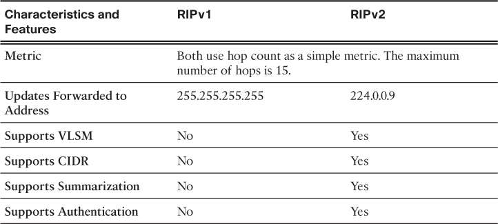
Table 3-5 summarizes the differences between RIPv1 and RIPv2.
RIP updates are encapsulated into a UDP segment, with both source and destination port numbers set to UDP port 520.
In 1997, the IPv6-enabled version of RIP was released. RIPng is based on RIPv2. It still has a 15-hop limitation and the administrative distance is 120.
Enhanced Interior Gateway Routing Protocol (3.2.2.2)
The Interior Gateway Routing Protocol (IGRP) was the first proprietary IPv4 routing protocol, developed by Cisco in 1984. It used the following design characteristics:
![]() Bandwidth, delay, load, and reliability are used to create a composite metric.
Bandwidth, delay, load, and reliability are used to create a composite metric.
![]() Routing updates are broadcast every 90 seconds, by default.
Routing updates are broadcast every 90 seconds, by default.
In 1992, IGRP was replaced by Enhanced IGRP (EIGRP). Like RIPv2, EIGRP also introduced support for VLSM and CIDR. EIGRP increases efficiency, reduces routing updates, and supports secure message exchange.
Table 3-6 summarizes the differences between IGRP and EIGRP.

EIGRP also introduced:
![]() Bounded triggered updates: It does not send periodic updates. Only routing table changes are propagated, whenever a change occurs. This reduces the amount of load the routing protocol places on the network. Bounded triggered updates means that EIGRP only sends to the neighbors that need it. It uses less bandwidth, especially in large networks with many routes.
Bounded triggered updates: It does not send periodic updates. Only routing table changes are propagated, whenever a change occurs. This reduces the amount of load the routing protocol places on the network. Bounded triggered updates means that EIGRP only sends to the neighbors that need it. It uses less bandwidth, especially in large networks with many routes.
![]() Hello keepalive mechanism: A small Hello message is periodically exchanged to maintain adjacencies with neighboring routers. This means a very low usage of network resources during normal operation, instead of the periodic updates.
Hello keepalive mechanism: A small Hello message is periodically exchanged to maintain adjacencies with neighboring routers. This means a very low usage of network resources during normal operation, instead of the periodic updates.
![]() Maintains a topology table: Maintains all the routes received from neighbors (not only the best paths) in a topology table. DUAL can insert backup routes into the EIGRP topology table.
Maintains a topology table: Maintains all the routes received from neighbors (not only the best paths) in a topology table. DUAL can insert backup routes into the EIGRP topology table.
![]() Rapid convergence: In most cases, it is the fastest IGP to converge because it maintains alternate routes, enabling almost instantaneous convergence. If a primary route fails, the router can use the alternate route identified. The switchover to the alternate route is immediate and does not involve interaction with other routers.
Rapid convergence: In most cases, it is the fastest IGP to converge because it maintains alternate routes, enabling almost instantaneous convergence. If a primary route fails, the router can use the alternate route identified. The switchover to the alternate route is immediate and does not involve interaction with other routers.
![]() Multiple network layer protocol support: EIGRP uses Protocol Dependent Modules (PDM), which means that it is the only protocol to include support for protocols other than IPv4 and IPv6, such as legacy IPX and AppleTalk.
Multiple network layer protocol support: EIGRP uses Protocol Dependent Modules (PDM), which means that it is the only protocol to include support for protocols other than IPv4 and IPv6, such as legacy IPX and AppleTalk.
![]() Packet Tracer Activity 3.2.2.4: Comparing RIP and EIGRP Path Selection
Packet Tracer Activity 3.2.2.4: Comparing RIP and EIGRP Path Selection
PCA and PCB need to communicate. The path that the data takes between these end devices can travel through R1, R2, and R3, or it can travel through R4 and R5. The process by which routers select the best path depends on the routing protocol. We will examine the behavior of two distance vector routing protocols, Enhanced Interior Gateway Routing Protocol (EIGRP) and Routing Information Protocol version 2 (RIPv2).
RIP and RIPng Routing (3.3)
Although the use of RIP has decreased in the past decade, it is still important to your networking studies because it might be encountered in a network implementation. As well, understanding how RIP operates and knowing its implementation will make learning other routing protocols easier.
Configuring the RIP Protocol (3.3.1)
In this section, you will learn how to configure, verify, and troubleshoot RIPv2.
Router RIP Configuration Mode (3.3.1.1)
Although RIP is rarely used in modern networks, it is useful as a foundation for understanding basic network routing. For this reason, this section provides a brief overview of how to configure basic RIP settings and to verify RIPv2.
Refer to the reference topology in Figure 3-22 and the addressing table in Table 3-7.


In this scenario, all routers have been configured with basic management features and all interfaces identified in the reference topology are configured and enabled. There are no static routes configured and no routing protocols enabled; therefore, remote network access is currently impossible. RIPv2 is used as the dynamic routing protocol.
To enable RIP, use the router rip command to enter router configuration mode, as shown in the following output. This command does not directly start the RIP process. Instead, it provides access to the router configuration mode where the RIP routing settings are configured.
R1# conf t
Enter configuration commands, one per line. End with CNTL/Z.
R1(config)# router rip
R1(config-router)#
To disable and eliminate RIP, use the no router rip global configuration command. This command stops the RIP process and erases all existing RIP configurations.
Figure 3-23 displays a partial list of the various RIP commands that can be configured. This section covers the two highlighted commands as well as network, passive-interface, and version.

Note
The entire output in Figure 3-23 can be viewed in the online course on page 3.3.1.1 graphic number 4.
Advertising Networks (3.3.1.2)
By entering the RIP router configuration mode, the router is instructed to run RIP. But the router still needs to know which local interfaces it should use for communication with other routers, as well as which locally connected networks it should advertise to those routers.
To enable RIP routing for a network, use the network network-address router configuration mode command. Enter the classful network address for each directly connected network. This command:
![]() Enables RIP on all interfaces that belong to a specific network. Associated interfaces now both send and receive RIP updates.
Enables RIP on all interfaces that belong to a specific network. Associated interfaces now both send and receive RIP updates.
![]() Advertises the specified network in RIP routing updates sent to other routers every 30 seconds.
Advertises the specified network in RIP routing updates sent to other routers every 30 seconds.
Note
If a subnet address is entered, the IOS automatically converts it to the classful network address. Remember RIPv1 is a classful routing protocol for IPv4. For example, entering the network 192.168.1.32 command would automatically be converted to network 192.168.1.0 in the running configuration file. The IOS does not give an error message, but instead corrects the input and enters the classful network address.
In the following command sequence, the network command is used to advertise the R1 directly connected networks.
R1(config)# router rip
R1(config-router)# network 192.168.1.0
R1(config-router)# network 192.168.2.0
R1(config-router)#
![]() Activity 3.3.1.2: Advertising the R2 and R3 Networks
Activity 3.3.1.2: Advertising the R2 and R3 Networks
Go to the online course to use the Syntax Checker in the second graphic to configure a similar configuration on R2 and R3.
Examining Default RIP Settings (3.3.1.3)
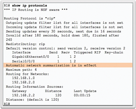
The output of the show ip protocols command in Figure 3-24 displays the IPv4 routing protocol settings currently configured on the router.

This output confirms that:
1. RIP routing is configured and running on router R1.
2. The values of various timers; for example, the next routing update is sent by R1 in 16 seconds.
3. The version of RIP configured is currently RIPv1.
4. R1 is currently summarizing at the classful network boundary.
5. The classful networks are advertised by R1. These are the networks that R1 includes in its RIP updates.
6. The RIP neighbors are listed, including their next-hop IP address, the associated AD that R2 uses for updates sent by this neighbor, and when the last update was received from this neighbor.
Note
This command is also very useful when verifying the operations of other routing protocols (i.e., EIGRP and OSPF).
The show ip route command displays the RIP routes installed in the routing table. In Figure 3-25, R1 now knows about the highlighted networks.
![]() Activity 3.3.1.3: Advertising the R2 and R3 Networks
Activity 3.3.1.3: Advertising the R2 and R3 Networks
Go to the online course to use the Syntax Checker in the third graphic to verify the R2 and R3 RIP settings and routes.
Enabling RIPv2 (3.3.1.4)
By default, when a RIP process is configured on a Cisco router, it is running RIPv1, as shown in the following output:
R1# show ip protocols
*** IP Routing is NSF aware ***
Routing Protocol is "rip"
Outgoing update filter list for all interfaces is not set
Incoming update filter list for all interfaces is not set
Sending updates every 30 seconds, next due in 16 seconds
Invalid after 180 seconds, hold down 180, flushed after 240
Redistributing: rip
Default version control: send version 1, receive any version
Interface Send Recv Triggered RIP Key-chain
GigabitEthernet0/0 1 1 2
Serial0/0/0 1 1 2
Automatic network summarization is in effect
Maximum path: 4
Routing for Networks:
192.168.1.0
192.168.2.0
Routing Information Sources:
Gateway Distance Last Update
192.168.2.2 120 00:00:15
Distance: (default is 120)
R1#
However, even though the router only sends RIPv1 messages, it can interpret both RIPv1 and RIPv2 messages. A RIPv1 router ignores the RIPv2 fields in the route entry.
Use the version 2 router configuration mode command to enable RIPv2, as shown in Figure 3-26.

Notice how the show ip protocols command verifies that R2 is now configured to send and receive version 2 messages only. The RIP process now includes the subnet mask in all updates, making RIPv2 a classless routing protocol.
Note
Configuring version 1 enables RIPv1 only, while configuring no version returns the router to the default setting of sending version 1 updates but listening for version 1 or version 2 updates.
The following output verifies that there are no RIP routes still in the routing table:
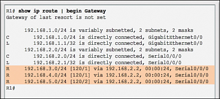
R1# show ip route | begin Gateway
Gateway of last resort is not set
192.168.1.0/24 is variably subnetted, 2 subnets, 2 masks
C 192.168.1.0/24 is directly connected, GigabitEthernet0/0
L 192.168.1.1/32 is directly connected, GigabitEthernet0/0
192.168.2.0/24 is variably subnetted, 2 subnets, 2 masks
C 192.168.2.0/24 is directly connected, Serial0/0/0
L 192.168.2.1/32 is directly connected, Serial0/0/0
R1#
There are no RIP routes because R1 is now only listening for RIPv2 updates. R2 and R3 are still sending RIPv1 updates. Therefore, the version 2 command must be configured on all routers in the routing domain.
![]() Activity 3.3.1.4: Enable and Verify RIPv2 on R2 and R3
Activity 3.3.1.4: Enable and Verify RIPv2 on R2 and R3
Go to the online course to use the Syntax Checker in the fourth graphic to enable RIPv2 on R2 and R3.
Disabling Auto Summarization (3.3.1.5)
As shown in Figure 3-27, RIPv2 automatically summarizes networks at major network boundaries by default, just like RIPv1.
To modify the default RIPv2 behavior of automatic summarization, use the no auto-summary router configuration mode command as shown in the following command sequence:
R1(config)# router rip
R1(config-router)# no auto-summary
R1(config-router)# end
R1#
*Mar 10 14:11:49.659: %SYS-5-CONFIG_I: Configured from console by console
R1# show ip protocols | section Automatic
Automatic network summarization is not in effect
R1#
This command has no effect when using RIPv1. When automatic summarization has been disabled, RIPv2 no longer summarizes networks to their classful address at boundary routers. RIPv2 now includes all subnets and their appropriate masks in its routing updates. The show ip protocols output now states that automatic network summarization is not in effect.
Note
RIPv2 must be enabled before automatic summarization is disabled.
![]() Activity 3.3.1.5: Disable Automatic Summarization on R2 and R3
Activity 3.3.1.5: Disable Automatic Summarization on R2 and R3
Go to the online course to use the Syntax Checker in the third graphic to disable automatic summarization on R2 and R3.
Configuring Passive Interfaces (3.3.1.6)
![]()
Passive Interfaces
By default, RIP updates are forwarded out all RIP-enabled interfaces. However, RIP updates really only need to be sent out interfaces connecting to other RIP-enabled routers.
For instance, refer to the topology in Figure 3-22. RIP sends updates out of its Gigabit Ethernet 0/0 interface even though no RIP device exists on that LAN. R1 has no way of knowing this and, as a result, sends an update every 30 seconds. Sending out unneeded updates on a LAN impacts the network in three ways:
![]() Wasted bandwidth: Bandwidth is used to transport unnecessary updates. Because RIP updates are either broadcasted or multicasted, switches also forward the updates out all ports.
Wasted bandwidth: Bandwidth is used to transport unnecessary updates. Because RIP updates are either broadcasted or multicasted, switches also forward the updates out all ports.
![]() Wasted resources: All devices on the LAN must process the update up to the transport layers, at which point the devices will discard the update.
Wasted resources: All devices on the LAN must process the update up to the transport layers, at which point the devices will discard the update.
![]() Security risk: Advertising updates on a broadcast network is a security risk. RIP updates can be intercepted with packet sniffing software. Routing updates can be modified and sent back to the router, corrupting the routing table with false metrics that misdirect traffic.
Security risk: Advertising updates on a broadcast network is a security risk. RIP updates can be intercepted with packet sniffing software. Routing updates can be modified and sent back to the router, corrupting the routing table with false metrics that misdirect traffic.
To address these problems, an interface can be configured to stop sending routing updates. This is referred to as configuring a passive interface. Use the passive-interface router configuration command to prevent the transmission of routing updates through a router interface but still allow that network to be advertised to other routers. The command stops routing updates out the specified interface. However, the network that the specified interface belongs to is still advertised in routing updates that are sent out other interfaces.
There is no need for R1, R2, and R3 to forward RIP updates out of their LAN interfaces. The configuration in Figure 3-28 identifies the R1 Gigabit Ethernet 0/0 interface as passive.

The show ip protocols command is then used to verify that the Gigabit Ethernet interface was passive. Notice that the Gigabit Ethernet 0/0 interface is no longer listed as sending or receiving version 2 updates, but instead is now listed under the Passive Interface(s) section. Also notice that the network 192.168.1.0 is still listed under Routing for Networks, which means that this network is still included as a route entry in RIP updates that are sent to R2.
Note
All routing protocols support the passive-interface command.
![]() Activity 3.3.1.6: Configuring and Verifying a Passive Interface on R2 and R3
Activity 3.3.1.6: Configuring and Verifying a Passive Interface on R2 and R3
Go to the online course to use the Syntax Checker in the third graphic to configure a passive interface on R2 and R3.
As an alternative, all interfaces can be made passive using the passive-interface default command. Interfaces that should not be passive can be re-enabled using the no passive-interface command.
Propagating a Default Route (3.3.1.7)
In the topology in Figure 3-29, R1 is single-homed to a service provider. Therefore, all that is required for R1 to reach the Internet is a default static route going out of the Serial 0/0/1 interface.

Similar default static routes could be configured on R2 and R3, but it is much more scalable to enter it one time on the edge router R1 and then have R1 propagate it to all other routers using RIP. To provide Internet connectivity to all other networks in the RIP routing domain, the default static route needs to be advertised to all other routers that use the dynamic routing protocol.
To propagate a default route, the edge router must be configured with:
![]() A default static route using the ip route 0.0.0.0 0.0.0.0 exit-intf next-hop-ip command.
A default static route using the ip route 0.0.0.0 0.0.0.0 exit-intf next-hop-ip command.
![]() The default-information originate router configuration command. This instructs R1 to originate default information, by propagating the static default route in RIP updates.
The default-information originate router configuration command. This instructs R1 to originate default information, by propagating the static default route in RIP updates.
The example in Figure 3-30 configures a fully specified default static route to the service provider, and then the route is propagated by RIP. Notice that R1 now has a Gateway of Last Resort and default route installed in its routing table.

![]() Activity 3.3.1.7: Verifying the Gateway of Last Resort on R2 and R3
Activity 3.3.1.7: Verifying the Gateway of Last Resort on R2 and R3
Go to the online course to use the Syntax Checker in the third graphic to verify that the default route has been propagated to R2 and R3.
![]() Packet Tracer Activity 3.3.1.8: Configuring RIPv2
Packet Tracer Activity 3.3.1.8: Configuring RIPv2
Although RIP is rarely used in modern networks, it is useful as a foundation for understanding basic network routing. In this activity, you will configure a default route, configure RIP version 2 with appropriate network statements and passive interfaces, and verify full connectivity.
Configuring the RIPng Protocol (3.3.2)
In this section, you will learn how to configure, verify, and troubleshoot RIPng.
Advertising IPv6 Networks (3.3.2.1)
As with its IPv4 counterpart, RIPng is rarely used in modern networks. It is also useful as a foundation for understanding basic network routing. For this reason, this section provides a brief overview of how to configure basic RIPng.
Refer to the reference topology in Figure 3-31.
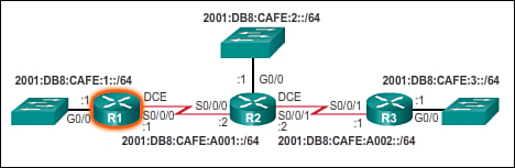
In this scenario, all routers have been configured with basic management features and all interfaces identified in the reference topology are configured and enabled. There are no static routes configured and no routing protocols enabled; therefore, remote network access is currently impossible.
To enable an IPv6 router to forward IPv6 packets, ipv6 unicast-routing must be configured.
Unlike RIPv2, RIPng is enabled on an interface and not in router configuration mode. In fact, there is no network network-address command available in RIPng. Instead, use the ipv6 rip domain-name enable interface configuration command.
In the following output, IPv6 unicast routing is enabled and the Gigabit Ethernet 0/0 and Serial 0/0/0 interfaces are enabled for RIPng using the domain name RIP-AS:
R1(config)# ipv6 unicast-routing
R1(config)#
R1(config)# interface gigabitethernet 0/0
R1(config-if)# ipv6 rip RIP-AS enable
R1(config-if)# exit
R1(config)#
R1(config)# interface serial 0/0/0
R1(config-if)# ipv6 rip RIP-AS enable
R1(config-if)# no shutdown
R1(config-if)#
![]() Activity 3.3.2.1: Enabling RIPng on the R2 and R3 Interfaces
Activity 3.3.2.1: Enabling RIPng on the R2 and R3 Interfaces
Go to the online course to use the Syntax Checker in the second graphic to enable RIPng on the R2 and R3 interfaces.
The process to propagate a default route in RIPng is identical to RIPv2 except that an IPv6 default static route must be specified. For example, assume that R1 had an Internet connection from a Serial 0/0/1 interface to IP address 2001:DB8:FEED:1::1/64. To propagate a default route, R1 would have to be configured with:
![]() A default static route using the ipv6 route 0::/0 2001:DB8:FEED:1::1 global configuration command.
A default static route using the ipv6 route 0::/0 2001:DB8:FEED:1::1 global configuration command.
![]() The ipv6 rip domain-name default-information originate interface configuration mode command. For example, the Serial 0/0/1 interface of R1 would have to be configured with the ipv6 rip RIP-AS default-information originate command. This would instruct R1 to be the source of the default route information and propagate the default static route in RIPng updates sent out of the RIPng-enabled interfaces.
The ipv6 rip domain-name default-information originate interface configuration mode command. For example, the Serial 0/0/1 interface of R1 would have to be configured with the ipv6 rip RIP-AS default-information originate command. This would instruct R1 to be the source of the default route information and propagate the default static route in RIPng updates sent out of the RIPng-enabled interfaces.
Examining the RIPng Configuration (3.3.2.2)
In Figure 3-32, the show ipv6 protocols command does not provide the same amount of information as its IPv4 counterpart.

However, the command does confirm the following parameters:
1. That RIPng routing is configured and running on router R1.
2. The interfaces configured with RIPng.
The show ipv6 route command displays the routes installed in the routing table as shown in Figure 3-33. The output confirms that R1 now knows about the highlighted RIPng networks.
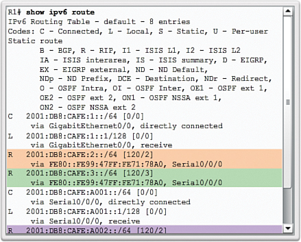
Notice that the R2 LAN is advertised as two hops away. This is because there is a difference in the way RIPv2 and RIPng calculate the hop counts. With RIPv2 (and RIPv1), the metric to the R2 LAN would be one hop. This is because the metric (hop count) that is displayed in the IPv4 routing table is the number of hops required to reach the remote network (counting the next-hop router as the first hop). In RIPng, the sending router already considers itself to be one hop away; therefore, R2 advertises its LAN with a metric of 1. When R1 receives the update, it adds another hop count of 1 to the metric. Therefore, R1 considers the R2 LAN to be two hops away. Similarly it considers the R3 LAN to be three hops away.
Appending the rip keyword to the command as shown in Figure 3-34 only lists RIPng networks.
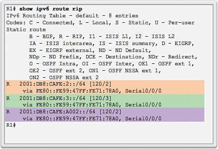
![]() Activity 3.3.2.2: Verifying RIPng Settings and Routes on R2 and R3
Activity 3.3.2.2: Verifying RIPng Settings and Routes on R2 and R3
Go to the online course to use the Syntax Checker in the fourth graphic to verify RIPng settings and routes on R2 and R3.
![]() Packet Tracer Activity 3.3.2.3: Configuring RIPng
Packet Tracer Activity 3.3.2.3: Configuring RIPng
RIPng (RIP Next Generation) is a distance vector routing protocol for routing IPv6 addresses. RIPng is based on RIPv2 and has the same administrative distance and 15-hop limitation. This activity will help you become more familiar with RIPng.
![]() Lab 3.3.2.4: Configuring RIPv2
Lab 3.3.2.4: Configuring RIPv2
In this lab, you will complete the following objectives:
![]() Part 1: Build the Network and Configure Basic Device Settings
Part 1: Build the Network and Configure Basic Device Settings
![]() Part 2: Configure and Verify RIPv2 Routing
Part 2: Configure and Verify RIPv2 Routing
![]() Part 3: Configure IPv6 on Devices
Part 3: Configure IPv6 on Devices
![]() Part 4: Configure and Verify RIPng Routing
Part 4: Configure and Verify RIPng Routing
Link-State Dynamic Routing (3.4)
Distance vector routing protocols are thought to be simple to understand, whereas link-state routing protocols have the reputation of being very complex, even intimidating. However, link-state routing protocols and concepts are not difficult to understand. In many ways, the link-state process is simpler to understand than distance vector concepts.
Link-State Routing Protocol Operation (3.4.1)
This section describes the characteristics, operations, and functionality of link-state routing protocols. Understanding the operation of link-state routing is critical to enabling, verifying, and troubleshooting these protocols.
Shortest Path First Protocols (3.4.1.1)
Link-state routing protocols are also known as shortest path first protocols and are built around Edsger Dijkstra’s shortest path first (SPF) algorithm. The SPF algorithm is discussed in more detail in a later section.
The IPv4 link-state routing protocols are shown Figure 3-35:
![]() Open Shortest Path First (OSPF)
Open Shortest Path First (OSPF)
![]() Intermediate System-to-Intermediate System (IS-IS)
Intermediate System-to-Intermediate System (IS-IS)
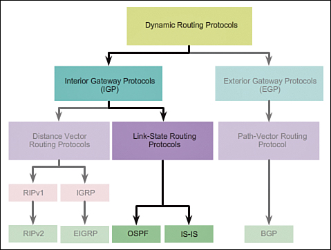
Link-state routing protocols have the reputation of being much more complex than their distance vector counterparts. However, the basic functionality and configuration of link-state routing protocols is equally straightforward.
Just like RIP and EIGRP, basic OSPF operations can be configured using the:
![]() router ospf process-id global configuration command
router ospf process-id global configuration command
![]() network command to advertise networks
network command to advertise networks
Dijkstra’s Algorithm (3.4.1.2)
![]()
Introduction to Dijkstra’s Algorithm
![]()
Dijkstra’s Algorithm Calculation
All link-state routing protocols apply Dijkstra’s algorithm to calculate the best path route. The algorithm is commonly referred to as the shortest path first (SPF) algorithm. This algorithm uses accumulated costs along each path, from source to destination, to determine the total cost of a route.
In Figure 3-36, each path is labeled with an arbitrary value for cost.

The cost of the shortest path for R2 to send packets to the LAN attached to R3 is 27. Specifically, the cost is R2 to R1 (20) plus R1 to R3 (5) plus R3 to LAN (2). Each router determines its own cost to each destination in the topology. In other words, each router calculates the SPF algorithm and determines the cost from its own perspective.
Note
The focus of this section is on cost, which is determined by the SPF tree. For this reason, the graphics throughout this section show the connections of the SPF tree, not the topology. All links are represented with a solid black line.
SPF Example (3.4.1.3)
The table in Figure 3-37 displays the shortest path and the accumulated cost to reach the identified destination networks from the perspective of R1.

The shortest path is not necessarily the path with the least number of hops. For example, look at the path to the R5 LAN. It might be assumed that R1 would send directly to R4 instead of to R3. However, the cost to reach R4 directly (22) is higher than the cost to reach R4 through R3 (17).
Observe the shortest path for each router to reach each of the LANs, as shown in Tables 3-8 through 3-11.
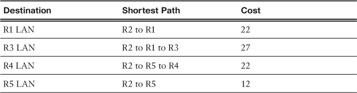
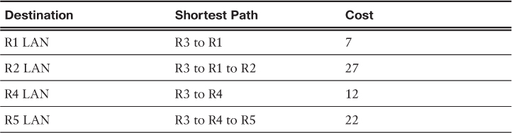
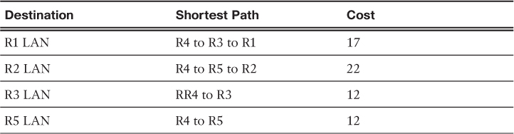

Link-State Updates (3.4.2)
Link-state updates (LSUs) are the packets used for OSPF routing updates. This section discusses how OSPF exchanges LSUs to discover the best routes.
Link-State Routing Process (3.4.2.1)
So exactly how does a link-state routing protocol work? With link-state routing protocols, a link is an interface on a router. Information about the state of those links is known as link-states.
All routers in an OSPF area will complete the following generic link-state routing process to reach a state of convergence:
1. Each router learns about its own links and its own directly connected networks. This is done by detecting that an interface is in the up state.
2. Each router is responsible for meeting its neighbors on directly connected networks. Link-state routers do this by exchanging Hello packets with other link-state routers on directly connected networks.
3. Each router builds a link-state packet (LSP)containing the state of each directly connected link. This is done by recording all the pertinent information about each neighbor, including neighbor ID, link type, and bandwidth.
4. Each router floods the LSP to all neighbors. Those neighbors store all LSPs received in a database. They then flood the LSPs to their neighbors until all routers in the area have received the LSPs. Each router stores a copy of each LSP received from its neighbors in a local database.
5. Each router uses the database to construct a complete map of the topology and computes the best path to each destination network. Like having a road map, the router now has a complete map of all destinations in the topology and the routes to reach them. The SPF algorithm is used to construct the map of the topology and to determine the best path to each network.
Note
This process is the same for both OSPF for IPv4 and OSPF for IPv6. The examples in this section refer to OSPF for IPv4.
Link and Link-State (3.4.2.2)
The first step in the link-state routing process is that each router learns about its own links, its own directly connected networks. When a router interface is configured with an IP address and subnet mask, the interface becomes part of that network.
Refer to the topology in Figure 3-38. For purposes of this discussion, assume that R1 was previously configured and had full connectivity to all neighbors. However, R1 lost power briefly and had to restart.
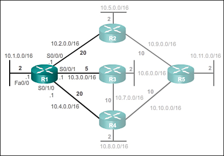
During boot up R1 loads the saved startup configuration file. As the previously configured interfaces become active, R1 learns about its own directly connected networks. Regardless of the routing protocols used, these directly connected networks are now entries in the routing table.
As with distance vector protocols and static routes, the interface must be properly configured with an IPv4 address and subnet mask, and the link must be in the up state before the link-state routing protocol can learn about a link. Also, like distance vector protocols, the interface must be included in one of the network router configuration statements before it can participate in the link-state routing process.
Figure 3-38 shows R1 linked to four directly connected networks:
![]() FastEthernet 0/0: 10.1.0.0/16
FastEthernet 0/0: 10.1.0.0/16
![]() Serial 0/0/0: 10.2.0.0/16
Serial 0/0/0: 10.2.0.0/16
![]() Serial 0/0/1: 10.3.0.0/16
Serial 0/0/1: 10.3.0.0/16
![]() Serial 0/1/0: 10.4.0.0/16
Serial 0/1/0: 10.4.0.0/16
As shown in Figures 3-39 through 3-42, the link-state information includes:
![]() The interface’s IPv4 address and subnet mask
The interface’s IPv4 address and subnet mask
![]() The type of network, such as Ethernet (broadcast) or Serial point-to-point link
The type of network, such as Ethernet (broadcast) or Serial point-to-point link
![]() The cost of that link
The cost of that link
![]() Any neighbor routers on that link
Any neighbor routers on that link


Note
Cisco’s implementation of OSPF specifies the OSPF routing metric as the cost of the link based on the bandwidth of the outgoing interface. For the purposes of this chapter, we are using arbitrary cost values to simplify the demonstration.
Say Hello (3.4.2.3)
The second step in the link-state routing process is that each router is responsible for meeting its neighbors on directly connected networks.
Routers with link-state routing protocols use a Hello protocol to discover any neighbors on their links. A neighbor is any other router that is enabled with the same link-state routing protocol.
In Figure 3-43, R1 sends Hello packets out its links (interfaces) to discover if there are any neighbors.

In Figure 3-44, R2, R3, and R4 reply to the Hello packet with their own Hello packets because these routers are configured with the same link-state routing protocol. There are no neighbors out the FastEthernet 0/0 interface. Because R1 does not receive a Hello on this interface, it does not continue with the link-state routing process steps for the FastEthernet 0/0 link.
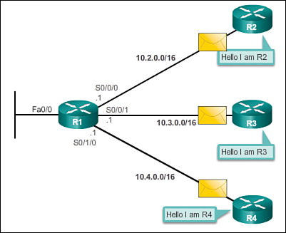
![]() Video 3.4.2.3: Neighbor Discovery—Hello Packets
Video 3.4.2.3: Neighbor Discovery—Hello Packets
Go to the online course and play the animation to view the link-state neighbor discovery process with Hello packets.
When two link-state routers learn that they are neighbors, they form an adjacency. These small Hello packets continue to be exchanged between two adjacent neighbors and serve as a keepalive function to monitor the state of the neighbor. If a router stops receiving Hello packets from a neighbor, that neighbor is considered unreachable and the adjacency is broken.
Building the Link-State Packet (3.4.2.4)
The third step in the link-state routing process is that each router builds an LSP containing the state of each directly connected link.
After a router has established its adjacencies, it can build its LSPs that contain the link-state information about its links. A simplified version of the LSP from R1 displayed in Figure 3-45 would contain the following:
1. R1; Ethernet network 10.1.0.0/16; Cost 2
2. R1 -> R2; Serial point-to-point network; 10.2.0.0/16; Cost 20
3. R1 -> R3; Serial point-to-point network; 10.3.0.0/16; Cost 5
4. R1 -> R4; Serial point-to-point network; 10.4.0.0/16; Cost 20
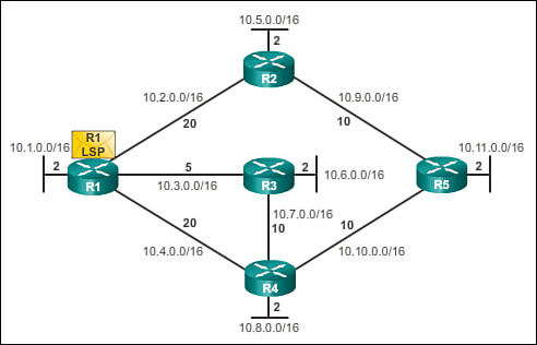
Flooding the LSP (3.4.2.5)
The fourth step in the link-state routing process is that each router floods the LSP to all neighbors, who then store all LSPs received in a database.
Each router floods its link-state information to all other link-state routers in the routing area as shown in Figure 3-46.

Whenever a router receives an LSP from a neighboring router, it immediately sends that LSP out all other interfaces except the interface that received the LSP. This process creates a flooding effect of LSPs from all routers throughout the routing area.
![]() Video 3.4.2.5: Routers Route Packets
Video 3.4.2.5: Routers Route Packets
Go to the online course and play the animation to view the LSP flooding.
In the animation, the LSPs are flooded almost immediately after being received without any intermediate calculations. Link-state routing protocols calculate the SPF algorithm after the flooding is complete. As a result, link-state routing protocols reach convergence very quickly.
Remember that LSPs do not need to be sent periodically. An LSP only needs to be sent:
![]() During initial startup of the routing protocol process on that router (e.g., router restart)
During initial startup of the routing protocol process on that router (e.g., router restart)
![]() Whenever there is a change in the topology (e.g., a link going down or coming up, a neighbor adjacency being established or broken)
Whenever there is a change in the topology (e.g., a link going down or coming up, a neighbor adjacency being established or broken)
In addition to the link-state information, other information is included in the LSP, such as sequence numbers and aging information, to help manage the flooding process. This information is used by each router to determine if it has already received the LSP from another router or if the LSP has newer information than what is already contained in the link-state database. This process allows a router to keep only the most current information in its link-state database.
Building the Link-State Database (3.4.2.6)
The final step in the link-state routing process is that each router uses the database to construct a complete map of the topology and computes the best path to each destination network.
Eventually, all routers receive an LSP from every other link-state router in the routing area. These LSPs are stored in the link-state database.
Table 3-12 displays the link-state database content of R1.
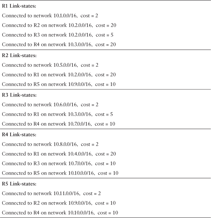
As a result of the flooding process, R1 has learned the link-state information for each router in its routing area. Notice that R1 also includes its own link-state information in the link-state database.
With a complete link-state database, R1 can now use the database and the shortest path first (SPF) algorithm to calculate the preferred path or shortest path to each network, resulting in the SPF tree.
Building the SPF Tree (3.4.2.7)
Each router in the routing area uses the link-state database and SPF algorithm to construct the SPF tree.
For example, using the link-state information from all other routers, R1 can now begin to construct an SPF tree of the network. To begin, the SPF algorithm interprets each router’s LSP to identify networks and associated costs.
The SPF algorithm then calculates the shortest paths to reach each individual network, resulting in the SPF tree as shown in Figure 3-47. R1 now has a complete topology view of the link-state area.

Note
The entire process can be viewed in the online course on page 3.4.2.7 in Figures 1 through 6.
Each router constructs its own SPF tree independently from all other routers. To ensure proper routing, the link-state databases used to construct those trees must be identical on all routers.
Adding OSPF Routes to the Routing Table (3.4.2.8)
Using the shortest path information determined by the SPF algorithm, these paths can now be added to the routing table. Figure 3-48 shows the routes that have now been added to R1’s IPv4 routing table.
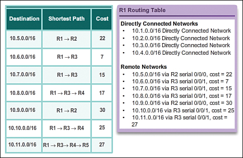
The routing table also includes all directly connected networks and routes from any other sources, such as static routes. Packets are now forwarded according to these entries in the routing table.
![]() Activity 3.4.2.9: Building the Link-State Database and SPF Tree
Activity 3.4.2.9: Building the Link-State Database and SPF Tree
Go to the online course to perform this practice activity.
Why Use Link-State Routing Protocols? (3.4.3)
This section discusses the advantages of using link-state routing protocols and compares the two types of link-state routing protocols.
Why Use Link-State Protocols? (3.4.3.1)
There are several advantages of link-state routing protocols compared to distance vector routing protocols.
![]() Builds a topological map: Link-state routing protocols create a topological map, or SPF tree of the network topology. Because link-state routing protocols exchange link-states, the SPF algorithm can build an SPF tree of the network. Using the SPF tree, each router can independently determine the shortest path to every network.
Builds a topological map: Link-state routing protocols create a topological map, or SPF tree of the network topology. Because link-state routing protocols exchange link-states, the SPF algorithm can build an SPF tree of the network. Using the SPF tree, each router can independently determine the shortest path to every network.
![]() Fast convergence: When receiving an LSP, link-state routing protocols immediately flood the LSP out all interfaces except for the interface from which the LSP was received. In contrast, RIP needs to process each routing update and update its routing table before flooding the routing update out other interfaces.
Fast convergence: When receiving an LSP, link-state routing protocols immediately flood the LSP out all interfaces except for the interface from which the LSP was received. In contrast, RIP needs to process each routing update and update its routing table before flooding the routing update out other interfaces.
![]() Event-driven updates: After the initial flooding of LSPs, link-state routing protocols only send out an LSP when there is a change in the topology. The LSP contains only the information regarding the affected link. Unlike some distance vector routing protocols, link-state routing protocols do not send periodic updates.
Event-driven updates: After the initial flooding of LSPs, link-state routing protocols only send out an LSP when there is a change in the topology. The LSP contains only the information regarding the affected link. Unlike some distance vector routing protocols, link-state routing protocols do not send periodic updates.
![]() Hierarchical design: Link-state routing protocols use the concept of areas. Multiple areas create a hierarchical design to networks, allowing for better route aggregation (summarization) and the isolation of routing issues within an area.
Hierarchical design: Link-state routing protocols use the concept of areas. Multiple areas create a hierarchical design to networks, allowing for better route aggregation (summarization) and the isolation of routing issues within an area.
Link-state protocols also have a few disadvantages compared to distance vector routing protocols:
![]() Memory requirements: Link-state protocols require additional memory to create and maintain the link-state database and SPF tree.
Memory requirements: Link-state protocols require additional memory to create and maintain the link-state database and SPF tree.
![]() Processing requirements: Link-state protocols can also require more CPU processing than distance vector routing protocols. The SPF algorithm requires more CPU time than distance vector algorithms such as Bellman-Ford, because link-state protocols build a complete map of the topology.
Processing requirements: Link-state protocols can also require more CPU processing than distance vector routing protocols. The SPF algorithm requires more CPU time than distance vector algorithms such as Bellman-Ford, because link-state protocols build a complete map of the topology.
![]() Bandwidth requirements: The flooding of link-state packets can adversely affect the available bandwidth on a network. This should only occur during initial startup of routers, but can also be an issue on unstable networks.
Bandwidth requirements: The flooding of link-state packets can adversely affect the available bandwidth on a network. This should only occur during initial startup of routers, but can also be an issue on unstable networks.
Link-State Protocols Support Multiple Areas (3.4.3.2)
Modern link-state routing protocols are designed to minimize the effects on memory, CPU, and bandwidth. The use and configuration of multiple areas can reduce the size of the link-state databases. Multiple areas can also limit the amount of link-state information flooding in a routing domain and send LSPs only to those routers that need them. When there is a change in the topology, only those routers in the affected area receive the LSP and run the SPF algorithm. This can help isolate an unstable link to a specific area in the routing domain.
For example, in Figure 3-49, there are three separate routing domains: area 1, area 0, and area 51.

If a network in area 51 goes down, the LSP with the information about this downed link is only flooded to other routers in that area. Only those routers in area 51 need to update their link-state databases, rerun the SPF algorithm, create a new SPF tree, and update their routing tables. Routers in other areas learn that this route is down, but this is done with a type of LSP that does not cause them to rerun their SPF algorithm. Routers in other areas can update their routing tables directly.
Protocols that Use Link-State (3.4.3.3)
There are only two link-state routing protocols, OSPF and IS-IS.
Open Shortest Path First (OSPF) is the most popular implementation. It was designed by the Internet Engineering Task Force (IETF) OSPF Working Group. The development of OSPF began in 1987 and there are two current versions in use:
![]() OSPFv2: OSPF for IPv4 networks (RFC 1247 and RFC 2328)
OSPFv2: OSPF for IPv4 networks (RFC 1247 and RFC 2328)
![]() OSPFv3: OSPF for IPv6 networks (RFC 2740)
OSPFv3: OSPF for IPv6 networks (RFC 2740)
IS-IS was designed by International Organization for Standardization (ISO) and is described in ISO 10589. The first incarnation of this routing protocol was developed at Digital Equipment Corporation (DEC) and is known as DECnet Phase V. Radia Perlman was the chief designer of the IS-IS routing protocol.
IS-IS was originally designed for the OSI protocol suite and not the TCP/IP protocol suite. Later, Integrated IS-IS, or Dual IS-IS, included support for IP networks. Although IS-IS has been known as the routing protocol used mainly by ISPs and carriers, more enterprise networks are beginning to use IS-IS.
OSPF and IS-IS share many similarities and also have many differences. There are many pro-OSPF and pro-IS-IS factions who discuss and debate the advantages of one routing protocol over the other. Both routing protocols provide the necessary routing functionality.
The Routing Table (3.5)
As a network administrator, it is important to know the routing table in depth when troubleshooting network issues. Understanding the structure and lookup process of the routing table will help you diagnose any routing table issue, regardless of your level of familiarity with a particular routing protocol. For example, you might encounter a situation in which the routing table has all of the routes you would expect to see, but packet forwarding is not performing as expected. Knowing how to step through the lookup process of a destination IP address for a packet will enable you to determine whether the packet is being forwarded as expected, if and why the packet is being sent elsewhere, or whether the packet has been discarded.
Parts of an IPv4 Route Entry (3.5.1)
A routing table consists of directly connected networks and routes learned statically or dynamically. This section examines these two types of routing table entries.
Routing Table Entries (3.5.1.1)
The topology displayed in Figure 3-50 is used as the reference topology for this section.

Notice that in the topology:
![]() R1 is the edge router that connects to the Internet. Therefore, it is propagating a default static route to R2 and R3.
R1 is the edge router that connects to the Internet. Therefore, it is propagating a default static route to R2 and R3.
![]() R1, R2, and R3 contain discontiguous networks separated by another classful network.
R1, R2, and R3 contain discontiguous networks separated by another classful network.
![]() R3 is also introducing a 192.168.0.0/16 supernet route.
R3 is also introducing a 192.168.0.0/16 supernet route.
Figure 3-51 displays the IPv4 routing table of R1 with directly connected, static, and dynamic routes.

Note
The routing table hierarchy in Cisco IOS was originally implemented with the classful routing scheme. Although the routing table incorporates both classful and classless addressing, the overall structure is still built around this classful scheme.
Directly Connected Entries (3.5.1.2)
As highlighted in Figure 3-52, the routing table of R1 contains three directly connected networks. Notice that two routing table entries are automatically created when an active router interface is configured with an IP address and subnet mask.

Figure 3-53 displays one of the routing table entries on R1 for the directly connected network 172.16.1.0. These entries were automatically added to the routing table when the GigabitEthernet 0/0 interface was configured and activated.

The entries contain the following information:
![]() Route source: Identifies how the route was learned. Directly connected interfaces have two route source codes. C identifies a directly connected network. Directly connected networks are automatically created whenever an interface is configured with an IP address and activated. L identifies that this is a local route. Local routes are automatically created whenever an interface is configured with an IP address and activated.
Route source: Identifies how the route was learned. Directly connected interfaces have two route source codes. C identifies a directly connected network. Directly connected networks are automatically created whenever an interface is configured with an IP address and activated. L identifies that this is a local route. Local routes are automatically created whenever an interface is configured with an IP address and activated.
![]() Destination network: The address of the remote network and how that network is connected.
Destination network: The address of the remote network and how that network is connected.
![]() Outgoing interface: Identifies the exit interface to use when forwarding packets to the destination network.
Outgoing interface: Identifies the exit interface to use when forwarding packets to the destination network.
Note
Local routing table entries did not appear in routing tables prior to IOS release 15.
A router typically has multiple interfaces configured. The routing table stores information about both directly connected and remote routes. As with directly connected networks, the route source identifies how the route was learned. For instance, common codes for remote networks include:
![]() S: Identifies that the route was manually created by an administrator to reach a specific network. This is known as a static route.
S: Identifies that the route was manually created by an administrator to reach a specific network. This is known as a static route.
![]() D: Identifies that the route was learned dynamically from another router using the EIGRP routing protocol.
D: Identifies that the route was learned dynamically from another router using the EIGRP routing protocol.
![]() O: Identifies that the route was learned dynamically from another router using the OSPF routing protocol.
O: Identifies that the route was learned dynamically from another router using the OSPF routing protocol.
![]() R: Identifies that the route was learned dynamically from another router using the RIP routing protocol.
R: Identifies that the route was learned dynamically from another router using the RIP routing protocol.
Remote Network Entries (3.5.1.3)
Figure 3-54 displays an IPv4 routing table entry on R1 for the route to remote network 172.16.4.0 on R3.

The entry identifies the following information:
![]() Route source: Identifies how the route was learned.
Route source: Identifies how the route was learned.
![]() Destination network: Identifies the address of the remote network.
Destination network: Identifies the address of the remote network.
![]() Administrative distance: Identifies the trustworthiness of the route source.
Administrative distance: Identifies the trustworthiness of the route source.
![]()
Administrative Distance
![]() Metric: Identifies the value assigned to reach the remote network. Lower values indicate preferred routes.
Metric: Identifies the value assigned to reach the remote network. Lower values indicate preferred routes.
![]()
Metric
![]() Next hop: Identifies the IPv4 address of the next router to forward the packet to.
Next hop: Identifies the IPv4 address of the next router to forward the packet to.
![]()
Next Hop Address
![]() Route timestamp: Identifies from when the route was last heard.
Route timestamp: Identifies from when the route was last heard.
![]() Outgoing interface: Identifies the exit interface to use to forward a packet toward the final destination.
Outgoing interface: Identifies the exit interface to use to forward a packet toward the final destination.
![]()
Lesson 7: Routing Protocol Characteristics
![]() Activity 3.5.1.4: Identify Parts of an IPv4 Routing Table Entry
Activity 3.5.1.4: Identify Parts of an IPv4 Routing Table Entry
Go to the online course to perform this practice activity.
Dynamically Learned IPv4 Routes (3.5.2)
The structure or format of the routing table might seem obvious until you take a closer look. Understanding the structure of the routing table will help you verify and troubleshoot routing issues because you will understand the routing table lookup process.
Routing Table Terms (3.5.2.1)
A dynamically built routing table provides a great deal of information, as shown in Figure 3-55. Therefore, it is crucial to understand the output generated by the routing table. Special terms are applied when discussing the contents of a routing table.

The Cisco IP routing table is not a flat database. The routing table is actually a hierarchical structure that is used to speed up the lookup process when locating routes and forwarding packets. Within this structure, the hierarchy includes several levels.
Routes are discussed in terms of:
![]() Ultimate route
Ultimate route
![]() Level 1 route
Level 1 route
![]() Level 1 parent route
Level 1 parent route
![]() Level 2 child routes
Level 2 child routes
Ultimate Route (3.5.2.2)
An ultimate route is a routing table entry that contains either a next-hop IPv4 address or an exit interface. Directly connected, dynamically learned, and local routes are ultimate routes.
In Figure 3-56, the highlighted areas are examples of ultimate routes. Notice that all of these routes specify either a next-hop IPv4 address or an exit interface.
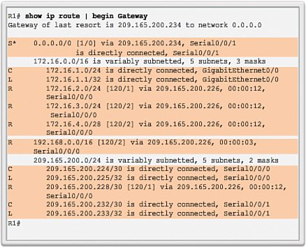
Level 1 Route (3.5.2.3)
A level 1 route is a route with a subnet mask equal to or less than the classful mask of the network address. Therefore, a level 1 route can be a:
![]() Network route: A network route has a subnet mask equal to that of the classful mask.
Network route: A network route has a subnet mask equal to that of the classful mask.
![]() Supernet route: A supernet route is a network address with a subnet mask less than the classful mask, for example, a summary address.
Supernet route: A supernet route is a network address with a subnet mask less than the classful mask, for example, a summary address.
![]() Default route: A default route is a static route with the address 0.0.0.0/0.
Default route: A default route is a static route with the address 0.0.0.0/0.
The source of the level 1 route can be a directly connected network, static route, or a dynamic routing protocol.
Figure 3-57 highlights how level 1 routes are also ultimate routes.
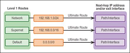
Figure 3-58 highlights level 1 routes.

Level 1 Parent Route (3.5.2.4)
As illustrated in Figure 3-59, a level 1 parent route is a level 1 network route that is subnetted. A parent route can never be an ultimate route.

Figure 3-60 highlights the level 1 parent routes in the routing table of R1. The routing table basically provides a heading for the specific subnets it contains. Each entry displays the classful network address, the number of subnets, and the number of different subnet masks that the classful address has been subdivided into.

Level 2 Child Route (3.5.2.5)
A level 2 child route is a route that is a subnet of a classful network address. As illustrated in Figure 3-61, a level 1 parent route is a level 1 network route that is subnetted.

A level 1 parent route contains level 2 child routes, as shown in Figure 3-62.
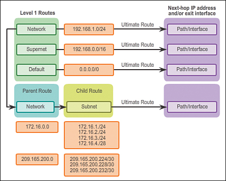
Like a level 1 route, the source of a level 2 route can be a directly connected network, a static route, or a dynamically learned route. Level 2 child routes are also ultimate routes.
Note
The routing table hierarchy in Cisco IOS has a classful routing scheme. A level 1 parent route is the classful network address of the subnet route. This is the case even if a classless routing protocol is the source of the subnet route.
Figure 3-63 highlights the level 2 child routes in the routing table of R1.
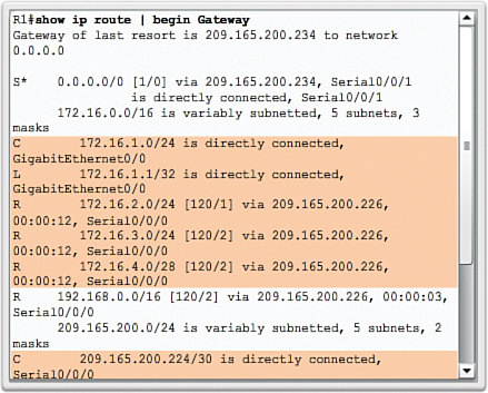
Note
The entire output in Figure 3-63 can be viewed in the online course on page 3.5.2.5 graphic number 3.
![]() Activity 3.5.2.6: Identify Parent and Child IPv4 Routes
Activity 3.5.2.6: Identify Parent and Child IPv4 Routes
Go to the online course to perform this practice activity.
The IPv4 Route Lookup Process (3.5.3)
Now that you understand the structure of the routing table, this section will help you understand the routing table lookup process.
Route Lookup Process (3.5.3.1)
When a packet arrives on a router interface, the router examines the IPv4 header, identifies the destination IPv4 address, and proceeds through the router lookup process.
In Figure 3-64, the router examines level 1 network routes for the best match with the destination address of the IPv4 packet.

Specifically, the router proceeds as follows:
1. If the best match is a level 1 ultimate route, then this route is used to forward the packet.
2. If the best match is a level 1 parent route, proceed to the next step.
In Figure 3-65, the router examines child routes (the subnet routes) of the parent route for a best match.

3. If there is a match with a level 2 child route, that subnet is used to forward the packet.
4. If there is not a match with any of the level 2 child routes, proceed to the next step.
In Figure 3-66, the router continues searching level 1 supernet routes in the routing table for a match, including the default route, if there is one.

5. If there is now a lesser match with a level 1 supernet or default routes, the router uses that route to forward the packet.
6. If there is not a match with any route in the routing table, the router drops the packet.
Note
A route referencing only a next-hop IP address and not an exit interface must be resolved to a route with an exit interface. A recursive lookup is performed on the next-hop IP address until the route is resolved to an exit interface.
Best Route = Longest Match (3.5.3.2)
What is meant by the router must find the best match in the routing table? Best match is equal to the longest match.
For there to be a match between the destination IPv4 address of a packet and a route in the routing table, a minimum number of far left bits must match between the IPv4 address of the packet and the route in the routing table. The subnet mask of the route in the routing table is used to determine the minimum number of far left bits that must match. Remember that an IPv4 packet only contains the IPv4 address and not the subnet mask.
The best match is the route in the routing table that has the most number of far left matching bits with the destination IPv4 address of the packet. The route with the greatest number of equivalent far left bits, or the longest match, is always the preferred route.
In Figure 3-67, a packet is destined for 172.16.0.10.

The router has three possible routes that match this packet: 172.16.0.0/12, 172.16.0.0/18, and 172.16.0.0/26. Of the three routes, 172.16.0.0/26 has the longest match and is therefore chosen to forward the packet. Remember, for any of these routes to be considered a match there must be at least the number of matching bits indicated by the subnet mask of the route.
![]() Activity 3.5.3.3: Determine the Longest Match Route
Activity 3.5.3.3: Determine the Longest Match Route
Go to the online course to perform this practice activity.
Analyze an IPv6 Routing Table (3.5.4)
The IPv6 routing table shares many similarities with the IPv4 routing table. It also consists of directly connected networks and routes learned statically or dynamically. However, the entries are displayed somewhat differently than IPv4 entries. This section examines the IPv6 routing table.
IPv6 Routing Table Entries (3.5.4.1)
Components of the IPv6 routing table are very similar to the IPv4 routing table. For instance, it is populated using directly connected interfaces, static routes, and dynamically learned routes.
Because IPv6 is classless by design, all routes are effectively level 1 ultimate routes. There is no level 1 parent of level 2 child routes.
The topology displayed in Figure 3-68 is used as the reference topology for this section.

Notice that in the topology:
![]() R1, R2, and R3 are configured in a full mesh topology. All routers have redundant paths to various networks.
R1, R2, and R3 are configured in a full mesh topology. All routers have redundant paths to various networks.
![]() R2 is the edge router and connects to the ISP; however, a default static route is not being advertised.
R2 is the edge router and connects to the ISP; however, a default static route is not being advertised.
![]() EIGRP for IPv6 has been configured on all three routers.
EIGRP for IPv6 has been configured on all three routers.
Directly Connected Entries (3.5.4.2)
The routing table of R1 is displayed in Figure 3-69 using the show ipv6 route command. Although the command output is displayed slightly differently than in the IPv4 version, it still contains the relevant route information.
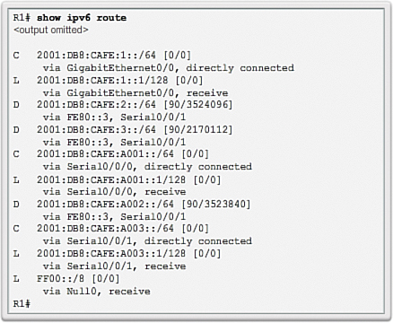
Figure 3-70 highlights the connected network and local routing table entries of the directly connected interfaces. The three entries were added when the interfaces were configured and activated.

As shown in Figure 3-71, directly connected route entries display the following information:
![]() Route source: Identifies how the route was learned. Directly connected interfaces have two route source codes (C identifies a directly connected network while L identifies that this is a local route).
Route source: Identifies how the route was learned. Directly connected interfaces have two route source codes (C identifies a directly connected network while L identifies that this is a local route).
![]() Directly connected network: The IPv6 address of the directly connected network.
Directly connected network: The IPv6 address of the directly connected network.
![]() Administrative distance: Identifies the trustworthiness of the route source. IPv6 uses the same distances as IPv4. A value of 0 indicates the best, most trustworthy source.
Administrative distance: Identifies the trustworthiness of the route source. IPv6 uses the same distances as IPv4. A value of 0 indicates the best, most trustworthy source.
![]() Metric: Identifies the value assigned to reach the remote network. Lower values indicate preferred routes.
Metric: Identifies the value assigned to reach the remote network. Lower values indicate preferred routes.
![]() Outgoing interface: Identifies the exit interface to use when forwarding packets to the destination network.
Outgoing interface: Identifies the exit interface to use when forwarding packets to the destination network.
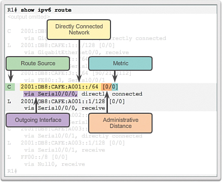
Note
The serial links have reference bandwidths configured to observe how EIGRP metrics select the best route. The reference bandwidth is not a realistic representation of modern networks. It is used only to provide a visual sense of link speed.
Remote IPv6 Network Entries (3.5.4.3)
Figure 3-72 highlights the routing table entries for the three remote networks (i.e., R2 LAN, R3 LAN, and the link between R2 and R3). The three entries were added by the EIGRP.

Figure 3-73 displays a routing table entry on R1 for the route to remote network 2001:DB8:CAFE:3::/64 on R3.

The entry identifies the following information:
![]() Route source: Identifies how the route was learned. Common codes include O (OSPF), D (EIGRP), R (RIP), and S (Static route).
Route source: Identifies how the route was learned. Common codes include O (OSPF), D (EIGRP), R (RIP), and S (Static route).
![]() Destination network: Identifies the address of the remote IPv6 network.
Destination network: Identifies the address of the remote IPv6 network.
![]() Administrative distance: Identifies the trustworthiness of the route source. IPv6 uses the same distances as IPv4.
Administrative distance: Identifies the trustworthiness of the route source. IPv6 uses the same distances as IPv4.
![]() Metric: Identifies the value assigned to reach the remote network. Lower values indicate preferred routes.
Metric: Identifies the value assigned to reach the remote network. Lower values indicate preferred routes.
![]() Next hop: Identifies the IPv6 address of the next router to forward the packet to.
Next hop: Identifies the IPv6 address of the next router to forward the packet to.
![]() Outgoing interface: Identifies the exit interface to use to forward a packet toward the final destination.
Outgoing interface: Identifies the exit interface to use to forward a packet toward the final destination.
When an IPv6 packet arrives on a router interface, the router examines the IPv6 header and identifies the destination IPv6 address. The router then proceeds through the following router lookup process.
The router examines level 1 network routes for the best match with the destination address of the IPv6 packet. Just like IPv4, the longest match is the best match. For example, if there are multiple matches in the routing table, the router chooses the route with the longest match. A match is made by matching the far left bits of the packet’s destination IPv6 address with the IPv6 prefix and prefix-length in the IPv6 routing table.
![]() Activity 3.5.4.4: Identify Parts of an IPv6 Routing Table Entry
Activity 3.5.4.4: Identify Parts of an IPv6 Routing Table Entry
Go to the online course to perform this practice activity.
Summary (3.6)
![]() Class Activity 3.6.1.1: IPv6 Details, Details...
Class Activity 3.6.1.1: IPv6 Details, Details...
After studying the concepts presented in this chapter concerning IPv6, you should be able to read a routing table easily and interpret the IPv6 routing information listed within it.
With a partner, use the IPv6 routing table diagram and the .pdf provided with this activity.
Record your answers to the Reflection questions.
Then compare your answers with, at least, one other group from the class.
Dynamic routing protocols are used by routers to facilitate the exchange of routing information between routers. The purpose of dynamic routing protocols includes: discovery of remote networks, maintaining up-to-date routing information, choosing the best path to destination networks, and ability to find a new best path if the current path is no longer available. While dynamic routing protocols require less administrative overhead than static routing, they do require dedicating part of a router’s resources for protocol operation, including CPU time and network link bandwidth.
Networks typically use a combination of both static and dynamic routing. Dynamic routing is the best choice for large networks and static routing is better for stub networks.
Routing protocols are responsible for discovering remote networks, as well as maintaining accurate network information. When there is a change in the topology, routing protocols propagate that information throughout the routing domain. The process of bringing all routing tables to a state of consistency, where all of the routers in the same routing domain or area have complete and accurate information about the network, is called convergence. Some routing protocols converge faster than others.
Routing protocols can be classified as either classful or classless, as distance vector or link-state, and as an Interior Gateway Protocol or an Exterior Gateway Protocol.
Distance vector protocols use routers as “sign posts” along the path to the final destination. The only information a router knows about a remote network is the distance or metric to reach that network and which path or interface to use to get there. Distance vector routing protocols do not have an actual map of the network topology.
A router configured with a link-state routing protocol can create a complete view or topology of the network by gathering information from all of the other routers.
Metrics are used by routing protocols to determine the best path or shortest path to reach a destination network. Different routing protocols may use different metrics. Typically, a lower metric means a better path. Metrics can be determined by hops, bandwidth, delay, reliability, and load.
Routers sometimes learn about multiple routes to the same network from both static routes and dynamic routing protocols. When a router learns about a destination network from more than one routing source, Cisco routers use the administrative distance value to determine which source to use. Each dynamic routing protocol has a unique administrative value, along with static routes and directly connected networks. The lower the administrative value, the more preferred the route source. A directly connected network is always the preferred source, followed by static routes and then various dynamic routing protocols.
The show ip protocols command displays the IPv4 routing protocol settings currently configured on the router. For IPv6, use show ipv6 protocols.
With link-state routing protocols such as OSPF, a link is an interface on a router. Information about the state of those links is known as link-states. All link-state routing protocols apply Dijkstra’s algorithm to calculate the best path route. The algorithm is commonly referred to as the shortest path first (SPF) algorithm. This algorithm uses accumulated costs along each path, from source to destination, to determine the total cost of a route.
Practice
The following activities provide practice with the topics introduced in this chapter. The Labs and Class Activities are available in the companion Routing Protocols Lab Manual (978-1-58713-322-0). The Packet Tracer Activities PKA files are found in the online course.
Class Activity 3.6.1.1: IPv6 Details, Details...
Packet Tracer Activity 3.2.2.4: Comparing RIP and EIGRP Path Selection
Packet Tracer Activity 3.3.1.8: Configuring RIPv2
Packet Tracer Activity 3.3.2.3: Configuring RIPng
Check Your Understanding Questions
Complete all the review questions listed here to test your understanding of the topics and concepts in this chapter. The appendix, “Answers to the ‘Check Your Understanding’ Questions,” lists the answers.
1. What are two advantages of static routing over dynamic routing? (Choose two.)
A. The configuration is less error prone.
B. Static routing is more secure because routers do not advertise routes.
C. Growing the network usually does not present a problem.
D. No computing overhead is involved.
E. The administrator has less work maintaining the configuration.
2. Match the description to the proper routing protocol.
Routing protocols:
RIP
IGRP
OSPF
EIGRP
BGP
Description:
A. Path vector exterior routing protocol:
B. Cisco advanced interior routing protocol:
C. Link-state interior routing protocol:
D. Distance vector interior routing protocol:
E. Cisco distance vector interior routing protocol:
3. Which statement best describes convergence on a network?
A. The amount of time required for routers to share administrative configuration changes, such as password changes, from one end of a network to the other end
B. The time required for the routers in the network to update their routing tables after a topology change has occurred
C. The time required for the routers in one autonomous system to learn routes to destinations in another autonomous system
D. The time required for routers running disparate routing protocols to update their routing tables
4. Dynamic routing protocols perform which two tasks? (Choose two.)
A. Assign IP addressing
B. Discover hosts
C. Network discovery
D. Propagate host default routes
E. Update and maintain routing tables
5. Which of the following parameters are used to calculate metrics? (Choose two.)
A. Hop count
B. Uptime
C. Bandwidth
D. Convergence time
E. Administrative distance
6. Which routing protocol has the most trustworthy administrative distance by default?
A. EIGRP internal routes
B. IS-IS
C. OSPF
D. RIPv1
E. RIPv2
7. Which command will show the administrative distance of routes?
A. show interfaces
B. show ip route
C. show ip interfaces
D. debug ip routing
8. When do directly connected networks appear in the routing table?
A. When they are included in a static route
B. When they are used as an exit interface
C. As soon as they are addressed and operational at Layer 2
D. As soon as they are addressed and operational at Layer 3
E. Always when a no shutdown command is issued
9. Router R1 is using the RIPv2 routing protocol and has discovered multiple unequal paths to reach a destination network. How will Router R1 determine which path is the best path to the destination network?
A. Lowest metric
B. Highest metric
C. Lowest administrative distance
D. Highest administrative distance
E. By load-balancing between up to four paths
10. Which of the following will trigger the sending of a link-state packet by OSPF? (Choose two.)
A. A change in the topology
B. A link to a neighbor router has become congested
C. The initial startup of the routing protocol process
D. The router update timer expiring
11. After examining its routing table for a best match with the destination address, which route will a router use to forward an IPv4 packet?
A. A level 1 child route
B. A level 1 parent route
C. A level 1 ultimate route
D. A level 2 supernet route
E. A level 2 parent route
12. What is different between IPv6 routing table entries and IPv4 routing table entries?
A. By design IPv6 is classless, so all routes are effectively level 1 ultimate routes.
B. Unlike IPv4, IPv6 does not use static routes to populate the routing table.
C. IPv6 routing tables include local route entries, which IPv4 routing tables do not.
D. The selection of IPv6 routes is based on the shortest matching prefix, unlike IPv4 route selection, which is based on the longest matching prefix.
13. Enter the proper administrative distance for each routing protocol.
A. eBGP:
B. EIGRP (Internal):
C. EIGRP (External):
D. IS-IS:
E. OSPF:
F. RIP:
14. Designate the following characteristics as belonging to either a classful routing protocol or a classless routing protocol.
A. Does not support discontiguous networks:
B. EIGRP, OSPF, and BGP:
C. Sends subnet mask information in routing updates:
D. Supports discontiguous networks:
E. RIP version 1 and IGRP:
F. Does not send subnet mask in its routing updates:
G. Allows for use of both 172.16.1.0/26 and 172.16.1.128/27 subnets in the same topology:
15. Explain why static routing might be preferred over dynamic routing.
16. What are four ways of classifying dynamic routing protocols?
17. What are the most common metrics used in IP dynamic routing protocols?
18. What is administrative distance, and why is it important?
19. What is the purpose of a passive interface?