Chapter 8. Multiarea OSPF
Objectives
Upon completion of this chapter, you will be able to answer the following questions:
![]() How do you explain why multiarea OSPF is used?
How do you explain why multiarea OSPF is used?
![]() How do you explain how multiarea OSPF uses link-state advertisements in order to maintain routing tables?
How do you explain how multiarea OSPF uses link-state advertisements in order to maintain routing tables?
![]() How do you explain how OSPF established neighbor adjacencies in a multiarea OSPF implementation?
How do you explain how OSPF established neighbor adjacencies in a multiarea OSPF implementation?
![]() How do you configure multiarea OSPFv2 and OSPFv3 in a routed network?
How do you configure multiarea OSPFv2 and OSPFv3 in a routed network?
![]() How do you configure multiarea OSPF route summarization in a routed network?
How do you configure multiarea OSPF route summarization in a routed network?
![]() How do you verify multiarea OSPFv2 and OSPFv3 operations?
How do you verify multiarea OSPFv2 and OSPFv3 operations?
Key Terms
This chapter uses the following key terms. You can find the definitions in the Glossary.
Autonomous System Boundary Router (ASBR)
Introduction (8.0.1.1)
Multiarea OSPF is used to divide a large OSPF network. Too many routers in one area increase the load on the CPU and create a large link-state database. In this chapter, directions are provided to effectively partition a large single area into multiple areas. Area 0 used in a single-area OSPF is known as the backbone area.
Discussion is focused on the LSAs exchanged between areas. In addition, activities for configuring OSPFv2 and OSPFv3 are provided. The chapter concludes with the show commands used to verify OSPF configurations.
![]() Class Activity 8.0.1.2: Leaving on a Jet Plane
Class Activity 8.0.1.2: Leaving on a Jet Plane
You and a classmate are starting a new airline to serve your continent.
In addition to your core area or headquarters airport, you will locate and map four intra-continental airport service areas and one transcontinental airport service area that can be used for additional source and destination travel.
Use the blank world map provided to design your airport locations. Additional instructions for completing this activity can be found in the accompanying PDF.
Multiarea OSPF Operation (8.1)
![]()
Multi-Area Configuration Example
In smaller networks with simple routing requirements, OSPF can be deployed in a single area with all routers in area 0. However, OSPF can scale to support the routing needs of large organizations by using a hierarchical, multiarea deployment. This section compares single-area and multiarea OSPF deployments and operation.
Single-Area OSPF (8.1.1.1)
Single-area OSPF is useful in smaller networks where the web of router links is not complex, and paths to individual destinations are easily deduced.
However, if an area becomes too big, the issues illustrated in Figure 8-1 must be addressed:
![]() Large routing table: OSPF does not perform route summarization by default. If the routes are not summarized, the routing table can become very large, depending on the size of the network.
Large routing table: OSPF does not perform route summarization by default. If the routes are not summarized, the routing table can become very large, depending on the size of the network.
![]() Large link-state database (LSDB): Because the LSDB covers the topology of the entire network, each router must maintain an entry for every network in the area, even if not every route is selected for the routing table.
Large link-state database (LSDB): Because the LSDB covers the topology of the entire network, each router must maintain an entry for every network in the area, even if not every route is selected for the routing table.
![]() Frequent SPF algorithm calculations: In a large network, changes are inevitable, so the routers spend many CPU cycles recalculating the SPF algorithm and updating the routing table.
Frequent SPF algorithm calculations: In a large network, changes are inevitable, so the routers spend many CPU cycles recalculating the SPF algorithm and updating the routing table.

To make OSPF more efficient and scalable, OSPF supports hierarchical routing using areas. An OSPF area is a group of routers that share the same link-state information in their link-state databases.
Multiarea OSPF (8.1.1.2)
When a large OSPF area is divided into smaller areas, this is called multiarea OSPF. Multiarea OSPF is useful in larger network deployments to reduce processing and memory overhead.
For instance, any time a router receives new information about the topology, as with additions, deletions, or modifications of a link, the router must rerun the SPF algorithm, create a new SPF tree, and update the routing table. The SPF algorithm is CPU-intensive and the time it takes for calculation depends on the size of the area. Too many routers in one area make the LSDB larger and increase the load on the CPU. Therefore, arranging routers into areas effectively partitions one potentially large database into smaller and more manageable databases.
Multiarea OSPF requires a hierarchical network design. The main area is called the backbone area (area 0) and all other areas must connect to the backbone area. With hierarchical routing, routing still occurs between the areas (interarea routing), while many of the tedious routing operations, such as recalculating the database, are kept within an area.
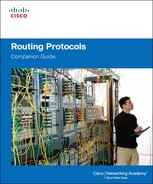
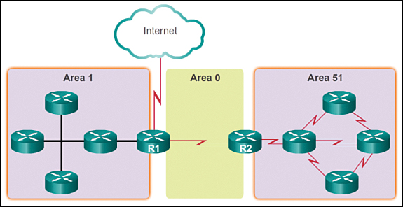
As illustrated in Figure 8-2, the hierarchical-topology possibilities of multiarea OSPF have these advantages:
![]() Smaller routing tables: There are fewer routing table entries, as network addresses can be summarized between areas. For example, R1 summarizes the routes from area 1 to area 0, and R2 summarizes the routes from area 51 to area 0. R1 and R2 also propagate a default static route to area 1 and area 51.
Smaller routing tables: There are fewer routing table entries, as network addresses can be summarized between areas. For example, R1 summarizes the routes from area 1 to area 0, and R2 summarizes the routes from area 51 to area 0. R1 and R2 also propagate a default static route to area 1 and area 51.
![]() Reduced link-state update overhead: Minimizes processing and memory requirements, because there are fewer routers exchanging LSAs.
Reduced link-state update overhead: Minimizes processing and memory requirements, because there are fewer routers exchanging LSAs.
![]() Reduced frequency of SPF calculations: Localizes impact of a topology change within an area. For instance, it minimizes routing update impact, because LSA flooding stops at the area boundary.
Reduced frequency of SPF calculations: Localizes impact of a topology change within an area. For instance, it minimizes routing update impact, because LSA flooding stops at the area boundary.
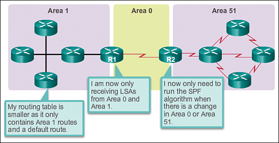
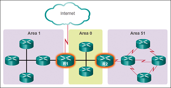
In Figure 8-3, the link between two internal routers fails in area 51. Notice that only the routers in area 51 exchange LSAs and rerun the SPF algorithm for this event. R1 does not receive LSAs from area 51 and does not recalculate the SPF algorithm.
OSPF Two-Layer Area Hierarchy (8.1.1.3)
Multiarea OSPF is implemented in a two-layer area hierarchy:
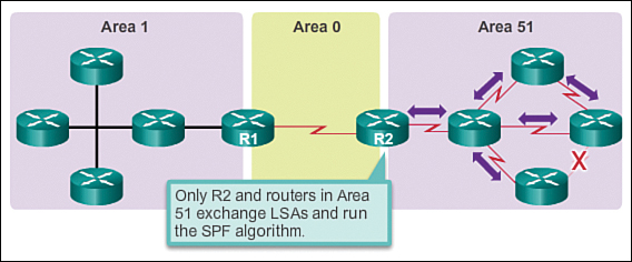
![]() Backbone (transit) area: The backbone area is an OSPF area whose primary function is the fast and efficient movement of IP packets. As shown in Figure 8-4, backbone areas interconnect with other OSPF areas. Generally, end users are not found within a backbone area. The backbone area is also called OSPF area 0. Hierarchical networking defines area 0 as the core to which all other areas directly connect.
Backbone (transit) area: The backbone area is an OSPF area whose primary function is the fast and efficient movement of IP packets. As shown in Figure 8-4, backbone areas interconnect with other OSPF areas. Generally, end users are not found within a backbone area. The backbone area is also called OSPF area 0. Hierarchical networking defines area 0 as the core to which all other areas directly connect.
![]() Regular (non-backbone) area: Regular areas are interconnected through the backbone area as shown in Figure 8-5. Regular areas connect users and resources. Regular areas are usually set up along functional or geographical groupings. By default, a regular area does not allow traffic from another area to use its links to reach other areas. All traffic from other areas must cross a transit area.
Regular (non-backbone) area: Regular areas are interconnected through the backbone area as shown in Figure 8-5. Regular areas connect users and resources. Regular areas are usually set up along functional or geographical groupings. By default, a regular area does not allow traffic from another area to use its links to reach other areas. All traffic from other areas must cross a transit area.
Note
A regular area can have a number of subtypes, including a standard area, stub area, totally stubby area, and not-so-stubby area (NSSA). Stub, totally stubby, and NSSAs are beyond the scope of this chapter.
OSPF enforces this rigid two-layer area hierarchy. The underlying physical connectivity of the network must map to the two-layer area structure, with all non-backbone areas attaching directly to area 0. All traffic moving from one area to another area must traverse the backbone area. This traffic is referred to as interarea traffic.
The optimal number of routers per area varies based on factors such as network stability, but Cisco recommends the following guidelines:
![]() An area should have no more than 50 routers.
An area should have no more than 50 routers.
![]() A router should not be in more than three areas.
A router should not be in more than three areas.
![]() Any single router should not have more than 60 neighbors.
Any single router should not have more than 60 neighbors.
Types of OSPF Routers (8.1.1.4)
OSPF routers of different types control the traffic that goes in and out of areas. The OSPF routers are categorized based on the function they perform in the routing domain.
There are four different types of OSPF routers:
![]() Internal router: As shown in Figure 8-6, internal routers have all of their interfaces in the same area. All internal routers in an area have identical LSDBs.
Internal router: As shown in Figure 8-6, internal routers have all of their interfaces in the same area. All internal routers in an area have identical LSDBs.

![]() Backbone router: As shown in Figure 8-7, backbone routers have at least one interface in area 0.
Backbone router: As shown in Figure 8-7, backbone routers have at least one interface in area 0.

![]() Area Border Router (ABR): As shown in Figure 8-8, an ABR has interfaces attached to multiple areas. It must maintain separate LSDBs for each area it is connected to, and can route between areas. ABRs are exit points for the area, which means that routing information destined for another area can get there only via the ABR of the local area. ABRs can be configured to summarize the routing information from the LSDBs of their attached areas. ABRs distribute the routing information into the backbone. The backbone routers then forward the information to the other ABRs. In a multiarea network, an area can have one or more ABRs.
Area Border Router (ABR): As shown in Figure 8-8, an ABR has interfaces attached to multiple areas. It must maintain separate LSDBs for each area it is connected to, and can route between areas. ABRs are exit points for the area, which means that routing information destined for another area can get there only via the ABR of the local area. ABRs can be configured to summarize the routing information from the LSDBs of their attached areas. ABRs distribute the routing information into the backbone. The backbone routers then forward the information to the other ABRs. In a multiarea network, an area can have one or more ABRs.
![]() Autonomous System Boundary Router (ASBR): As shown in Figure 8-9, an ASBR has at least one interface attached to an external internetwork (another autonomous system), such as a non-OSPF network. An ASBR can import non-OSPF network information to the OSPF network, and vice versa, using a process called route redistribution.
Autonomous System Boundary Router (ASBR): As shown in Figure 8-9, an ASBR has at least one interface attached to an external internetwork (another autonomous system), such as a non-OSPF network. An ASBR can import non-OSPF network information to the OSPF network, and vice versa, using a process called route redistribution.

Redistribution in multiarea OSPF occurs when an ASBR connects different routing domains (e.g., EIGRP and OSPF) and configures them to exchange and advertise routing information between those routing domains.
A router can be classified as more than one router type. For example, if a router connects to area 0 and area 1 and in addition maintains routing information for another, non-OSPF network, it falls under three different classifications: a backbone router, an ABR, and an ASBR.
![]() Activity 8.1.1.5: Identify the Multiarea OSPF Terminology
Activity 8.1.1.5: Identify the Multiarea OSPF Terminology
Go to the online course to perform this practice activity.
Multiarea OSPF LSA Operation (8.1.2)
In this section, you will learn how multiarea OSPF exchanges special LSAs to provide interarea information.
OSPF LSA Types (8.1.2.1)
LSAs are the building blocks of the OSPF LSDB. Individually, they act as database records and provide specific OSPF network details. In combination, they describe the entire topology of an OSPF network or area.
The RFCs for OSPF currently specify up to 11 different LSA types, as listed and described in Table 8-1. However, any implementation of multiarea OSPF must support the first five LSAs: LSA 1 to LSA 5. The focus of this section is on these first five LSAs.

Each router link is defined as an LSA type. The LSA includes a link ID field that identifies, by network number and mask, the object to which the link connects. Depending on the type, the link ID has different meanings. LSAs differ on how they are generated and propagated within the routing domain.
Note
OSPFv3 includes additional LSA types.
OSPF LSA Type 1 (8.1.2.2)
As shown in Figure 8-10, all routers advertise their directly connected OSPF-enabled links in a type 1 router LSA and forward their network information to OSPF neighbors. The LSA contains a list of the directly connected interfaces, link types, and link states.

Type 1 LSAs are also referred to as router link entries. They include a list of directly connected network prefixes and link types. All routers generate type 1 LSAs.
Type 1 LSAs are flooded only within the area in which they originate and do not propagate beyond an ABR. ABRs subsequently advertise the networks learned from the type 1 LSAs to other areas as type 3 LSAs.
The type 1 LSA link ID is identified by the router ID of the originating router.
OSPF LSA Type 2 (8.1.2.3)
A type 2 network LSA only exists for multiaccess and nonbroadcast multiaccess (NBMA) networks where there is a DR elected and at least two routers on the multiaccess segment. The type 2 network LSA contains the router ID and IP address of the DR, along with the router ID of all other routers on the multiaccess segment. A type 2 LSA is created for every multiaccess network in the area.
Type 2 LSAs are also referred to as network link entries. The purpose of a type 2 LSA is to give other routers information about multiaccess networks within the same area. Type 2 LSAs identify the routers and the network addresses of the multiaccess links.
Only a DR generates a type 2 LSA. The DR floods type 2 LSAs only within the area in which they originated. Type 2 LSAs are not forwarded outside of an area. The link-state ID for a network LSA is the IP interface address of the DR that advertises it.
As shown in Figure 8-11, ABR1 is the DR for the Ethernet network in area 1. It generates the type 2 LSA and forwards it into area 1. ABR2 is the DR for the multiaccess network in area 0. There are no multiaccess networks in area 2 and, therefore, no type 2 LSAs are ever propagated in that area.
OSPF LSA Type 3 (8.1.2.4)
Type 3 summary LSAs are used by ABRs to advertise networks from other areas. ABRs collect type 1 LSAs in the LSDB. After an OSPF area has converged, the ABR creates a type 3 LSA for each of its learned OSPF networks. Therefore, an ABR with many OSPF routes must create type 3 LSAs for each network.
As shown in Figure 8-12, ABR1 and ABR2 flood type 3 LSAs from one area to other areas. The ABRs propagate the type 3 LSAs into other areas.
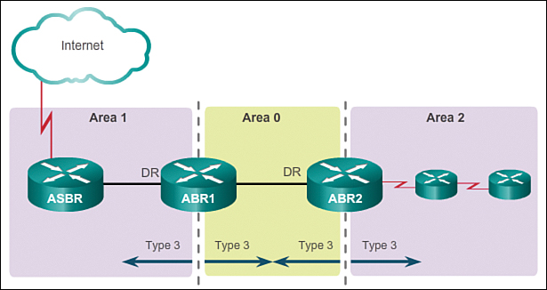
By default, routes are not summarized. In a large OSPF deployment with many networks, propagating type 3 LSAs can cause significant flooding problems. For this reason, it is strongly recommended that manual route summarization be configured on the ABR.
ABRs flood type 3 LSAs to other areas and are regenerated by other ABRs. A type 3 LSA link-state ID is identified by the network address.
Receiving a type 3 LSA into its area does not cause a router to run the SPF algorithm. The routes being advertised in the type 3 LSAs are appropriately added to or deleted from the router’s routing table, but a full SPF calculation is not necessary.
OSPF LSA Type 4 (8.1.2.5)
Type 4 and type 5 LSAs are used collectively to identify an ASBR and advertise external networks into an OSPF routing domain.
A type 4 summary LSA is generated by an ABR only when an ASBR exists within an area. Type 4 LSAs are used to advertise an ASBR to other areas and provide a route to the ASBR. All traffic destined to an external autonomous system requires routing table knowledge of the ASBR that originated the external routes. A type 4 LSA is generated by the originating ABR and is regenerated by other ABRs.
As shown in Figure 8-13, the ASBR sends a type 1 LSA, identifying itself as an ASBR. The LSA includes a special bit known as the external bit (e bit) that is used to identify the router as an ASBR. When ABR1 receives the type 1 LSA, it notices the e bit, builds a type 4 LSA, and then floods the type 4 LSA to the backbone (area 0). Subsequent ABRs flood the type 4 LSA into other areas.

The link-state ID is set to the ASBR router ID.
OSPF LSA Type 5 (8.1.2.6)
Type 5 external LSAs describe routes to networks outside the OSPF autonomous system. Type 5 LSAs are originated by the ASBR and are flooded to the entire autonomous system and regenerated by other ABRs. A type 5 LSA link-state ID is the external network address.
Type 5 LSAs are also referred to as autonomous system external LSA entries.
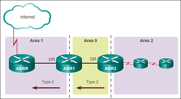
In Figure 8-14, the ASBR generates type 5 LSAs for each of its external routes and floods them into the area. Subsequent ABRs also flood the type 5 LSA into other areas. Routers in other areas use the information from the type 4 LSA to reach the external routes.

By default, external routes are not summarized. In a large OSPF deployment with many networks, propagating multiple type 5 LSAs can cause significant flooding problems. For this reason, it is strongly recommended that manual route summarization be configured on the ASBR.
![]() Activity 8.1.2.7: Identify the OSPF LSA Type
Activity 8.1.2.7: Identify the OSPF LSA Type
Go to the online course to perform this practice activity.
OSPF Routing Table and Types of Routes (8.1.3)
Multiarea OSPF uses special route descriptors to indicate routes learned from other areas. In this section, you will learn about these descriptors and their meaning.
OSPF Routing Table Entries (8.1.3.1)
Figure 8-15 provides a sample routing table for a multiarea OSPF topology with a link to an external non-OSPF network.

OSPF routes in an IPv4 routing table are identified using the following descriptors:
![]() O: Router (type 1) and network (type 2) LSAs describe the details within an area. The routing table reflects this link-state information with a designation of O, meaning that the route is intra-area.
O: Router (type 1) and network (type 2) LSAs describe the details within an area. The routing table reflects this link-state information with a designation of O, meaning that the route is intra-area.
![]() O IA: When an ABR receives summary LSAs, it adds them to its LSDB and regenerates them into the local area. The internal routers then assimilate the information into their databases. Summary LSAs appear in the routing table as IA (interarea) routes.
O IA: When an ABR receives summary LSAs, it adds them to its LSDB and regenerates them into the local area. The internal routers then assimilate the information into their databases. Summary LSAs appear in the routing table as IA (interarea) routes.
![]() O E1 or O E2: When an ABR receives external LSAs, it adds them to its LSDB and floods them into the area. External LSAs appear in the routing table marked as external type 1 (E1) or external type 2 (E2) routes.
O E1 or O E2: When an ABR receives external LSAs, it adds them to its LSDB and floods them into the area. External LSAs appear in the routing table marked as external type 1 (E1) or external type 2 (E2) routes.
Figure 8-16 displays an IPv6 routing table with OSPF router, interarea, and external routing table entries.

OSPF Route Calculation (8.1.3.2)
Each router uses the SPF algorithm against the LSDB to build the SPF tree. The SPF tree is used to determine the best paths.
As shown in Figure 8-17, the order in which the best paths are calculated is as follows:
1. All routers calculate the best paths to destinations within their area (intra-area) and add these entries to the routing table. These are the type 1 and type 2 LSAs, which are noted in the routing table with a routing designator of O. (1)
2. All routers calculate the best paths to the other areas within the internetwork. These best paths are the interarea route entries, or type 3 and type 4 LSAs, and are noted with a routing designator of O IA. (2)
3. All routers (except those that are in a form of stub area) calculate the best paths to the external autonomous system (type 5) destinations. These are noted with either an O E1 or an O E2 route designator, depending on the configuration. (3)

When converged, a router can communicate with any network within or outside the OSPF autonomous system.
![]() Activity 8.1.3.3: Order the Steps for OSPF Best Path Calculations
Activity 8.1.3.3: Order the Steps for OSPF Best Path Calculations
Go to the online course to perform this practice activity.
Configuring Multiarea OSPF (8.2)
Configuring multiarea OSPF is similar to configuring single-area OSPF. In this section, you will learn how to configure multiarea OSPF.
Implementing Multiarea OSPF (8.2.1.1)
OSPF can be implemented as single-area or multiarea. The type of OSPF implementation to choose depends on the specific requirements and existing topology.
There are four steps to implementing multiarea OSPF. Steps 1 and 2 are part of the planning process.
The steps to implement multiarea OSPF are:
Step 1. Gather the network requirements and parameters. This includes determining the number of host and network devices, the IP addressing scheme (if already implemented), the size of the routing domain, the size of the routing tables, the risk of topology changes, and other network characteristics.
Step 2. Define the OSPF parameters. Based on information gathered during Step 1, the network administrator must determine if single-area or multiarea OSPF is the preferred implementation. If multiarea OSPF is selected, there are several considerations the network administrator must take into account while determining the OSPF parameters, to include:
![]() IP addressing plan: This governs how OSPF can be deployed and how well the OSPF deployment might scale. A detailed IP addressing plan, along with the IP subnetting information, must be created. A good IP addressing plan should enable the usage of OSPF multiarea design and summarization. This plan more easily scales the network, as well as optimizes OSPF behavior and the propagation of LSAs.
IP addressing plan: This governs how OSPF can be deployed and how well the OSPF deployment might scale. A detailed IP addressing plan, along with the IP subnetting information, must be created. A good IP addressing plan should enable the usage of OSPF multiarea design and summarization. This plan more easily scales the network, as well as optimizes OSPF behavior and the propagation of LSAs.
![]() OSPF areas: Dividing an OSPF network into areas decreases the LSDB size and limits the propagation of link-state updates when the topology changes. The routers that are to be ABRs and ASBRs must be identified, as those are to perform any summarization or redistribution.
OSPF areas: Dividing an OSPF network into areas decreases the LSDB size and limits the propagation of link-state updates when the topology changes. The routers that are to be ABRs and ASBRs must be identified, as those are to perform any summarization or redistribution.
![]() Network topology: This consists of links that connect the network equipment and belong to different OSPF areas in a multiarea OSPF design. Network topology is important to determine primary and backup links. Primary and backup links are defined by the changing OSPF cost on interfaces. A detailed network topology plan should also be used to determine the different OSPF areas, ABR, and ASBR as well as summarization and redistribution points, if multiarea OSPF is used.
Network topology: This consists of links that connect the network equipment and belong to different OSPF areas in a multiarea OSPF design. Network topology is important to determine primary and backup links. Primary and backup links are defined by the changing OSPF cost on interfaces. A detailed network topology plan should also be used to determine the different OSPF areas, ABR, and ASBR as well as summarization and redistribution points, if multiarea OSPF is used.
Step 3. Configure the multiarea OSPF implementation based on the parameters.
Step 4. Verify the multiarea OSPF implementation based on the parameters.
Configuring Multiarea OSPF (8.2.1.2)
Figure 8-18 displays the reference OSPFv2 multiarea topology.

In this example:
![]() R1 is an ABR because it has interfaces in area 1 and an interface in area 0.
R1 is an ABR because it has interfaces in area 1 and an interface in area 0.
![]() R2 is an internal backbone router because all of its interfaces are in area 0.
R2 is an internal backbone router because all of its interfaces are in area 0.
![]() R3 is an ABR because it has interfaces in area 2 and an interface in area 0.
R3 is an ABR because it has interfaces in area 2 and an interface in area 0.
There are no special commands required to implement this multiarea OSPF network. A router simply becomes an ABR when it has two network statements in different areas.
As shown in the following example, R1 is assigned the router ID 1.1.1.1. This example enables OSPF on the two LAN interfaces in area 1. The serial interface is configured as part of OSPF area 0. Because R1 has interfaces connected to two different areas, it is an ABR.
R1(config)# router ospf 10
R1(config-router)# router-id 1.1.1.1
R1(config-router)# network 10.1.1.1 0.0.0.0 area 1
R1(config-router)# network 10.1.2.1 0.0.0.0 area 1
R1(config-router)# network 192.168.10.1 0.0.0.0 area 0
R1(config-router)# end
R1#
![]() Activity 8.2.1.2: Configuring Multiarea OSPF on R2 and R3
Activity 8.2.1.2: Configuring Multiarea OSPF on R2 and R3
Go to the online course to use the Syntax Checker in the third graphic to configure multiarea OSPF on R2 and R3. In this Syntax Checker, on R2, use the wildcard mask of the interface network address. On R3, use the 0.0.0.0 wildcard mask for all networks.
Configuring Multiarea OSPFv3 (8.2.1.3)
Figure 8-19 displays the reference OSPFv3 multiarea topology.

As with OSPFv2, implementing the multiarea OSPFv3 topology shown in Figure 8-19 is simple. There are no special commands required. A router simply becomes an ABR when it has two interfaces in different areas.
In the following example, R1 is assigned the router ID 1.1.1.1. The example also enables OSPF on the LAN interface in area 1 and the serial interface in area 0. Because R1 has interfaces connected to two different areas, it becomes an ABR.
R1(config)# ipv6 router ospf 10
R1(config-rtr)# router-id 1.1.1.1
R1(config-rtr)# exit
R1(config)#
R1(config)# interface GigabitEthernet 0/0
R1(config-if)# ipv6 ospf 10 area 1
R1(config-if)#
R1(config-if)# interface Serial0/0/0
R1(config-if)# ipv6 ospf 10 area 0
R1(config-if)# end
R1#
![]() Activity 8.2.1.3: Configuring Multiarea OSPFv3 on R2 and R3
Activity 8.2.1.3: Configuring Multiarea OSPFv3 on R2 and R3
Go to the online course to use the Syntax Checker in the third graphic to configure multiarea OSPFv3 on R2 and on R3.
OSPF Route Summarization (8.2.2.1)
Summarization helps keep routing tables small. It involves consolidating multiple routes into a single advertisement, which can then be propagated into the backbone area.
Normally, type 1 and type 2 LSAs are generated inside each area, translated into type 3 LSAs, and sent to other areas. If area 1 had 30 networks to advertise, then 30 type 3 LSAs would be forwarded into the backbone. With route summarization, the ABR consolidates the 30 networks into one or two advertisements.
In Figure 8-20, R1 consolidates all of the network advertisements into one summary LSA. Instead of forwarding individual LSAs for each route in area 1, R1 forwards a summary LSA to the core router C1. C1, in turn, forwards the summary LSA to R2 and R3. R2 and R3 then forward it to their respective internal routers.

Summarization also helps increase the network’s stability, because it reduces unnecessary LSA flooding. This directly affects the amount of bandwidth, CPU, and memory resources consumed by the OSPF routing process. Without route summarization, every specific-link LSA is propagated into the OSPF backbone and beyond, causing unnecessary network traffic and router overhead.
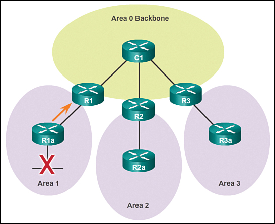
In Figure 8-21, a network link on R1a fails. R1a sends an LSA to R1. However, R1 does not propagate the update, because it has a summary route configured. Specific-link LSA flooding outside the area does not occur.
Interarea and External Route Summarization (8.2.2.2)
In OSPF, summarization can only be configured on ABRs or ASBRs. Instead of advertising many specific networks, the ABR routers and ASBR routers can advertise a summary route. ABR routers can summarize type 3 LSAs and ASBR routers can summarize type 5 LSAs.
By default, summary LSAs (type 3 LSAs) and external LSAs (type 5 LSAs) do not contain summarized (aggregated) routes; that is, by default, summary LSAs are not summarized.
Route summarization can be configured as follows:
![]() Interarea route summarization: As shown in Figure 8-22, interarea route summarization occurs on ABRs and applies to routes from within each area. It does not apply to external routes injected into OSPF via redistribution. To perform effective interarea route summarization, network addresses within areas should be assigned contiguously so that these addresses can be summarized into a minimal number of summary addresses.
Interarea route summarization: As shown in Figure 8-22, interarea route summarization occurs on ABRs and applies to routes from within each area. It does not apply to external routes injected into OSPF via redistribution. To perform effective interarea route summarization, network addresses within areas should be assigned contiguously so that these addresses can be summarized into a minimal number of summary addresses.

Note
Interarea route summarization is configured on ABRs using the area area-id range address mask router configuration mode command.
![]() External route summarization: External route summarization is specific to external routes that are injected into OSPF via route redistribution. Again, it is important to ensure the contiguity of the external address ranges that are being summarized. Generally, only ASBRs summarize external routes. As shown in Figure 8-23, EIGRP external routes are summarized by ASBR R2 in a single LSA and sent to R1 and R3.
External route summarization: External route summarization is specific to external routes that are injected into OSPF via route redistribution. Again, it is important to ensure the contiguity of the external address ranges that are being summarized. Generally, only ASBRs summarize external routes. As shown in Figure 8-23, EIGRP external routes are summarized by ASBR R2 in a single LSA and sent to R1 and R3.

Note
External route summarization is configured on ASBRs using the summary-address address mask router configuration mode command.
Interarea Route Summarization (8.2.2.3)
OSPF does not perform auto-summarization. Interarea summarization must be manually configured on ABRs.
Summarization of internal routes can only be done by ABRs. When summarization is enabled on an ABR, it injects into the backbone a single type 3 LSA describing the summary route. Multiple routes inside the area are summarized by the one LSA.
A summary route is generated if at least one subnet within the area falls in the summary address range. The summarized route metric is equal to the lowest cost of all subnets within the summary address range.
Note
An ABR can only summarize routes that are within the areas connected to the ABR.
Figure 8-24 shows a multiarea OSPF topology.

The routing tables of R1 and R3 are examined to see the effect of the summarization. Figure 8-25 displays the R1 routing table before summarization is configured.
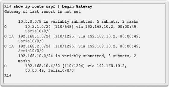
Figure 8-26 displays the R3 routing table. Notice how R3 currently has two interarea entries to the R1 area 1 networks.

Calculating the Summary Route (8.2.2.4)
Summarizing networks into a single address and mask can be done in three steps:
Step 1. List the networks in binary format.
Step 2. Count the number of far left matching bits to determine the mask for the summary route.
Step 3. Copy the matching bits and then add zero bits to determine the summarized network address.
Refer to Figure 8-27 for an example on how to calculate a summary route.

In the example, the two R1 area 1 networks 10.1.1.0/24 and 10.1.2.0/24 are listed in binary format. As highlighted, the first 22 far left matching bits match. This results in the prefix /22 or subnet mask 255.255.252.0. The matching bits with zeros at the end result in a network address of 10.1.0.0/22. This summary address summarizes four networks: 10.1.0.0/24, 10.1.1.0/24, 10.1.2.0/24, and 10.1.3.0/24. In the example the summary address matches four networks although only two networks exist.
Configuring Interarea Route Summarization (8.2.2.5)
To manually configure interarea route summarization on an ABR, use the area area-id range address mask router configuration mode command. This instructs the ABR to summarize routes for a specific area before injecting them into a different area, via the backbone as type 3 summary LSAs.
Note
In OSPFv3, the command is identical except for the IPv6 network address. The command syntax for OSPFv3 is area area-id range prefix/prefix-length.
The following summarizes the two internal area 1 routes on R1 into one OSPF interarea summary route. The summarized route 10.1.0.0/22 actually summarizes four network addresses, 10.1.0.0/24 to 10.1.3.0/24.
R1(config)# router ospf 10
R1(config-router)# area 1 range 10.1.0.0 255.255.252.0
R1(config-router)#
Figure 8-28 displays the IPv4 routing table of R1. Notice how a new entry has appeared with a Null0 exit interface. The Cisco IOS automatically creates a summary route to the Null0 interface when manual summarization is configured to prevent routing loops. A packet sent to a null interface is dropped.

For example, assume R1 received a packet destined for 10.1.0.10. Although it would match the R1 summary route, R1 does not have a valid route in area 1. Therefore, R1 would refer to the routing table for the next longest match, which would be the Null0 entry. The packet would get forwarded to the Null0 interface and dropped. This prevents the router from forwarding the packet to a default route and possibly creating a routing loop.
Figure 8-29 displays the updated R3 routing table. Notice how there is now only one interarea entry going to the summary route 10.1.0.0/22. Although this example only reduced the routing table by one entry, summarization could be implemented to summarize many networks. This would reduce the size of routing tables.

![]() Activity 8.2.2.5: Summarizing Area 2 Routes
Activity 8.2.2.5: Summarizing Area 2 Routes
Go to the online course to use the Syntax Checker in the fifth graphic to summarize the area 2 routes on R3.
Verifying Multiarea OSPF (8.2.3.1)
The same verification commands used to verify single-area OSPF also can be used to verify multiarea OSPF:
![]() show ip ospf neighbor
show ip ospf neighbor
![]() show ip ospf
show ip ospf
![]() show ip ospf interface
show ip ospf interface
Commands that verify specific multiarea information include:
![]() show ip protocols
show ip protocols
![]() show ip ospf interface brief
show ip ospf interface brief
![]() show ip route ospf
show ip route ospf
![]() show ip ospf database
show ip ospf database
Note
For the equivalent OSPFv3 command, simply substitute ip with ipv6.
Verify General Multiarea OSPF Settings (8.2.3.2)
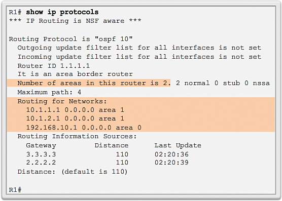
Use the show ip protocols command to verify the OSPF status. The output of the command reveals which routing protocols are configured on a router. It also includes routing protocol specifics such as the router ID, number of areas in the router, and networks included within the routing protocol configuration.
Figure 8-30 displays the OSPF settings of R1. Notice that the command shows that there are two areas. The “Routing for Networks” section of the output identifies the networks and their respective areas.
Use the show ip ospf interface brief command to display concise OSPF-related information of OSPF-enabled interfaces. This command reveals useful information, such as the OSPF process ID that the interface is assigned to, the area that the interfaces are in, and the cost of the interface.
Figure 8-31 verifies the OSPF-enabled interfaces and the areas to which they belong.

![]() Activity 8.2.3.2: Verifying Multiarea OSPF Status
Activity 8.2.3.2: Verifying Multiarea OSPF Status
Go to the online course to use the Syntax Checker in the third graphic to verify general settings on R2 and R3.
Verify the OSPF Routes (8.2.3.3)
The most common command used to verify a multiarea OSPF configuration is the show ip route command. Add the ospf parameter to display only OSPF-related information.
Figure 8-32 displays the routing table of R1.

Notice how the O IA entries in the routing table identify networks learned from other areas. Specifically, O represents OSPF intra-area routes, and IA represents interarea, which means that the route originated from another area. Recall that R1 is in area 0, and the 192.168.1.0 and 192.168.2.0 subnets are connected to R3 in area 2. The [110/1295] entry in the routing table represents the administrative distance that is assigned to OSPF (110) and the total cost of the routes (cost of 1295).
![]() Activity 8.2.3.3: Verifying Multiarea OSPF Routes on R2 and R3
Activity 8.2.3.3: Verifying Multiarea OSPF Routes on R2 and R3
Go to the online course to use the Syntax Checker in the second graphic to verify the routing table of R2 and R3 using the show ip route ospf command.
Verify the Multiarea OSPF LSDB (8.2.3.4)
Use the show ip ospf database command to verify the contents of the LSDB.
There are many command options available with the show ip ospf database command.
For example, Figure 8-33 displays the content of the LSDB of R1.

Notice R1 has entries for area 0 and area 1, because ABRs must maintain a separate LSDB for each area to which they belong. In the output, “Router Link States” in area 0 identifies three routers. The “Summary Net Link States” section identifies networks learned from other areas and which neighbor advertised the network.
![]() Activity 8.2.3.4: Verify the OSPF LSDB on R2 and R3
Activity 8.2.3.4: Verify the OSPF LSDB on R2 and R3
Go to the online course to use the Syntax Checker in the second graphic to verify the LSDB of R2 and R3 using the show ip ospf database command. R2 only has interfaces in area 0; therefore, only one LSDB is required. Like R1, R3 contains two LSDBs.
Verify Multiarea OSPFv3 (8.2.3.5)
Like OSPFv2, OSPFv3 provides similar OSPFv3 verification commands. Refer to the reference OSPFv3 topology in Figure 8-34.

The following output displays the OSPFv3 settings of R1. Notice that the command confirms that there are now two areas. It also identifies each interface enabled for the respective area.
R1# show ipv6 protocols
IPv6 Routing Protocol is "connected"
IPv6 Routing Protocol is "ND"
IPv6 Routing Protocol is "ospf 10"
Router ID 1.1.1.1
Area border router
Number of areas: 2 normal, 0 stub, 0 nssa
Interfaces (Area 0):
Serial0/0/0
Interfaces (Area 1):
GigabitEthernet0/0
Redistribution:
None
R1#
Figure 8-35 verifies the OSPFv3-enabled interfaces and the area to which they belong.

Figure 8-36 displays the routing table of R1. Notice how the IPv6 routing table displays OI entries in the routing table to identify networks learned from other areas. Specifically, O represents OSPF intra-area routes, and I represents interarea, which means that the route originated from another area. Recall that R1 is in area 0, and the 2001:DB8:CAFE3::/64 subnet is connected to R3 in area 2. The [110/1295] entry in the routing table represents the administrative distance that is assigned to OSPF (110) and the total cost of the routes (cost of 1295).
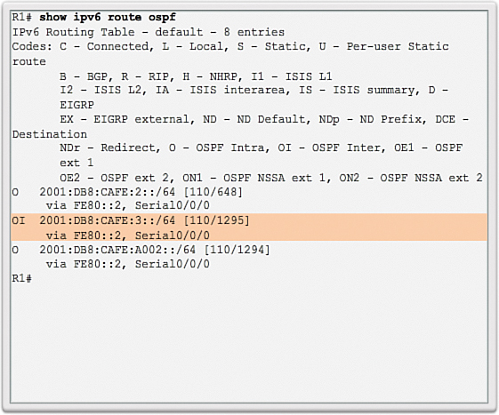
Figure 8-37 displays the content of the LSDB of R1. The command offers similar information to its OSPFv2 counterpart. However, the OSPFv3 LSDB contains additional LSA types not available in OSPFv2.
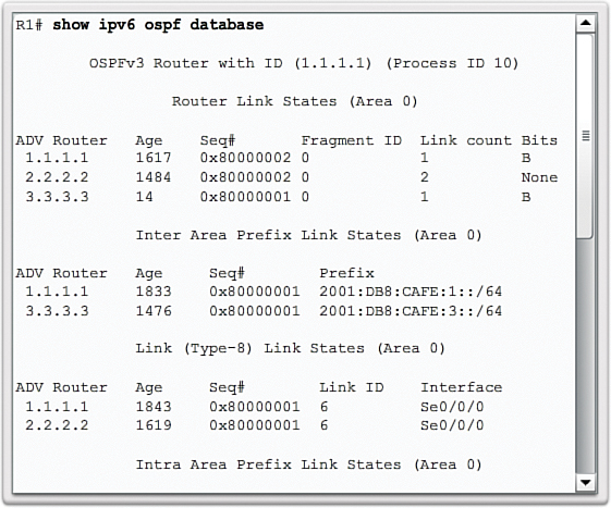
Note
The entire output in Figure 8-37 can be viewed in the online course on page 8.2.3.5 graphic number 5.
![]() Packet Tracer Activity 8.2.3.6: Configuring Multiarea OSPFv2
Packet Tracer Activity 8.2.3.6: Configuring Multiarea OSPFv2
In this activity, you will configure multiarea OSPFv2. The network is already connected and interfaces are configured with IPv4 addressing. Your job is to enable multiarea OSPFv2, verify connectivity, and examine the operation of multiarea OSPFv2.
![]() Packet Tracer Activity 8.2.3.7: Configuring Multiarea OSPFv3
Packet Tracer Activity 8.2.3.7: Configuring Multiarea OSPFv3
In this activity, you will configure multiarea OSPFv3. The network is already connected and interfaces are configured with IPv6 addressing. Your job is to enable multiarea OSPFv3, verify connectivity, and examine the operation of multiarea OSPFv3
![]() Lab 8.2.3.8: Configuring Multiarea OSPFv2
Lab 8.2.3.8: Configuring Multiarea OSPFv2
In this lab, you will complete the following objectives:
![]() Part 1: Build the Network and Configure Basic Device Settings
Part 1: Build the Network and Configure Basic Device Settings
![]() Part 2: Configure a Multiarea OSPFv2 Network
Part 2: Configure a Multiarea OSPFv2 Network
![]() Part 3: Configure Interarea Summary Routes
Part 3: Configure Interarea Summary Routes
![]() Lab 8.2.3.9: Configuring Multiarea OSPFv3
Lab 8.2.3.9: Configuring Multiarea OSPFv3
In this lab, you will complete the following objectives:
![]() Part 1: Build the Network and Configure Basic Device Settings
Part 1: Build the Network and Configure Basic Device Settings
![]() Part 2: Configure a Multiarea OSPFv3 Network
Part 2: Configure a Multiarea OSPFv3 Network
![]() Part 3: Configure Interarea Route Summarization
Part 3: Configure Interarea Route Summarization
![]() Lab 8.2.3.10: Troubleshooting Multiarea OSPF
Lab 8.2.3.10: Troubleshooting Multiarea OSPF
In this lab, you will complete the following objectives:
Part 1: Build the Network and Load Device Configurations
Part 2: Troubleshoot Layer 3 Connectivity
Part 3: Troubleshoot OSPFv2
Part 4: Troubleshoot OSPFv3
Summary (8.3)
![]() Class Activity 8.3.1.1: Digital Trolleys
Class Activity 8.3.1.1: Digital Trolleys
Your city has an aging digital trolley system based on a one-area design. All communications within this one area are taking longer to process as trolleys are being added to routes serving the population of your growing city. Trolley departures and arrivals are also taking a little longer, because each trolley must check large routing tables to determine where to pick up and deliver residents from their source and destination streets.
A concerned citizen has come up with the idea of dividing the city into different areas for a more efficient way to determine trolley routing information. It is thought that if the trolley maps are smaller, the system might be improved because of faster and smaller updates to the routing tables.
Your city board approves and implements the new area-based, digital trolley system. But to ensure the new area routes are more efficient, the city board needs data to show the results at the next open board meeting.
Complete the directions found in the PDF for this activity. Share your answers with your class.
Single-area OSPF is useful in smaller networks but in larger networks multiarea OSPF is a better choice. Multiarea OSPF solves the issues of large routing table, large link-state database, and frequent SPF algorithm calculations.
The main area is called the backbone area (area 0) and all other areas must connect to the backbone area. Routing still occurs between the areas while many of the routing operations, such as recalculating the database, are kept within an area.
There are four different types of OSPF routers: internal router, backbone router, Area Border Router (ABR), and Autonomous System Boundary Router (ASBR). A router can be classified as more than one router type.
Link-state advertisements (LSAs) are the building blocks of OSPF. This chapter concentrated on LSA type 1 to LSA type 5. Type 1 LSAs are referred to as the router link entries. Type 2 LSAs are referred to as the network link entries and are flooded by a DR. Type 3 LSAs are referred to as the summary link entries and are created and propagated by ABRs. A type 4 summary LSA is generated by an ABR only when an ASBR exists within an area. Type 5 external LSAs describe routes to networks outside the OSPF autonomous system. Type 5 LSAs are originated by the ASBR and are flooded to the entire autonomous system.
OSPF routes in an IPv4 routing table are identified using the following descriptors: O, O IA, O E1, or O E2. Each router uses the SPF algorithm against the LSDB to build the SPF tree. The SPF tree is used to determine the best paths.
There are no special commands required to implement a multiarea OSPF network. A router simply becomes an ABR when it has two network statements in different areas.
An example of multiarea OSPF configuration:
R1(config)# router ospf 10
R1(config-router)# router-id 1.1.1.1
R1(config-router)# network 10.1.1.1 0.0.0.0 area 1
R1(config-router)# network 10.1.2.1 0.0.0.0 area 1
R1(config-router)# network 192.168.10.1 0.0.0.0 area 0
OSPF does not perform auto-summarization. In OSPF, summarization can only be configured on ABRs or ASBRs. Interarea route summarization must be manually configured and occurs on ABRs and applies to routes from within each area. To manually configure interarea route summarization on an ABR, use the area area-id range address mask router configuration mode command.
External route summarization is specific to external routes that are injected into OSPF via route redistribution. Generally, only ASBRs summarize external routes. External route summarization is configured on ASBRs using the summary-address address mask router configuration mode command.
Commands that are used to verify OSPF configuration consist of the following:
![]() show ip ospf neighbor
show ip ospf neighbor
![]() show ip ospf
show ip ospf
![]() show ip ospf interface
show ip ospf interface
![]() show ip protocols
show ip protocols
![]() show ip ospf interface brief
show ip ospf interface brief
![]() show ip route ospf
show ip route ospf
![]() show ip ospf database
show ip ospf database
Practice
The following activities provide practice with the topics introduced in this chapter. The Labs and Class Activities are available in the companion Routing Protocols Lab Manual (978-1-58713-322-0). The Packet Tracer Activities PKA files are found in the online course.
Class Activity 8.3.1.1: Digital Trolleys
Lab 8.2.3.9: Configuring Multiarea OSPFv3
Lab 8.2.3.10: Troubleshooting Multiarea OSPF
Packet Tracer Activity 8.2.3.7: Configuring Multiarea OSPFv3
Check Your Understanding Questions
Complete all the review questions listed here to test your understanding of the topics and concepts in this chapter. The appendix, “Answers to the ‘Check Your Understanding’ Questions,” lists the answers.
1. Which statement describes a multiarea OSPF network?
A. Consists of multiple network areas that are daisy-chained together.
B. It has a core backbone area with other areas connected to the backbone area.
C. It has multiple routers that run multiple routing protocols simultaneously, and each protocol consists of an area.
D. It requires a three-layer hierarchical network design approach.
2. What is one advantage of using multiarea OSPF?
A. It allows OSPFv2 and OSPFv3 to exchange routing updates.
B. It enables multiple routing protocols to be running in a large network.
C. It improves the routing efficiency by reducing the routing table and link-state update overhead.
D. It increases the routing performance by dividing the neighbor table into separate smaller ones.
3. Which characteristic describes ABRs and ASBRs implemented in a multiarea OSPF network?
A. They are required to perform any summarization or redistribution tasks.
B. They are required to reload frequently and quickly in order to update the LSDB.
C. They both run multiple routing protocols simultaneously.
D. They usually have many local networks attached.
4. An ABR in a multiarea OSPF network receives LSAs from its neighbor that identify the neighbor as an ASBR with learned external networks from the Internet. Which LSA type would the ABR send to other areas to identify the ASBR, so that internal traffic that is destined for the Internet will be sent through the ASBR??
A. LSA type 1
B. LSA type 2
C. LSA type 3
D. LSA type 4
E. LSA type 5
5. Which two statements correctly describe OSPF type 3 LSAs? (Choose two.)
A. Type 3 LSAs are generated without requiring a full SPF calculation.
B. Type 3 LSAs are known as autonomous system external LSA entries.
C. Type 3 LSAs are known as router link entries.
D. Type 3 LSAs are used for routes to networks outside the OSPF autonomous system.
E. Type 3 LSAs are used to update routes between OSPF areas.
6. What can be concluded about a routing table entry with a route source of “O”?
A. The route entry was learned from an ABR.
B. The route entry was learned from an ASBR.
C. The route entry was learned from an internal router in another area.
D. The route entry was learned from an internal router in the same area.
7. What can be concluded about a routing table entry with a route source of “O IA”?
A. The route entry was learned from an ABR.
B. The route entry was learned from an ASBR.
C. The route entry was learned from an internal router in another area.
D. The route entry was learned from an internal router in the same area.
8. What can be concluded about a routing table entry with a route source of “O*E2”?
A. The route entry was learned from an ABR.
B. The route entry was learned from an ASBR.
C. The route entry was learned from an internal router in another area.
D. The route entry was learned from an internal router in the same area.
9. Which statement is true regarding an ABR?
A. It can also be an internal router.
B. It is a router with all of its interfaces in the same area.
C. It is a router with at least one interface attached in a non-OSPF network.
D. It is a router with interfaces attached to multiple areas.
10. Which statement is true regarding an ASBR?
A. It can also be an internal router.
B. It is a router in the backbone area.
C. It is a router with all of its interfaces in the same area.
D. It is a router with at least one interface attached in a non-OSPF network.
E. It is a router with interfaces attached to multiple areas.