Chapter 6. Single-Area OSPF
Objectives
Upon completion of this chapter, you will be able to answer the following questions:
![]() What is the process by which link-state routers learn about other networks?
What is the process by which link-state routers learn about other networks?
![]() How do you describe the types of packets used by Cisco IOS routers to establish and maintain an OSPF network?
How do you describe the types of packets used by Cisco IOS routers to establish and maintain an OSPF network?
![]() How do you explain how Cisco IOS routers achieve convergence in an OSPF network?
How do you explain how Cisco IOS routers achieve convergence in an OSPF network?
![]() How do you configure an OSPF router ID?
How do you configure an OSPF router ID?
![]() How do you configure single-area OSPFv2 in a small, routed IPv4 network?
How do you configure single-area OSPFv2 in a small, routed IPv4 network?
![]() How does OSPF use cost to determine the best path?
How does OSPF use cost to determine the best path?
![]() How do you verify single-area OSPFv2 in a small, routed network?
How do you verify single-area OSPFv2 in a small, routed network?
![]() How do you describe the characteristics and operations of OSPFv2 and OSPFv3?
How do you describe the characteristics and operations of OSPFv2 and OSPFv3?
![]() How do you configure single-area OSPFv3 in a small, routed IPv6 network?
How do you configure single-area OSPFv3 in a small, routed IPv6 network?
![]() How do you verify single-area OSPFv3 in a small, routed network?
How do you verify single-area OSPFv3 in a small, routed network?
Key Terms
This chapter uses the following key terms. You can find the definitions in the Glossary.
Open Shortest Path First (OSPF) classless
link-state advertisements (LSAs)
Database Description (DBD) packet
Link-State Request (LSR) packet
Link-State Update (LSU) packet
Link-State Acknowledgment (LSAck)
nonbroadcast multi-access (NBMA) networks
Backup Designated Router (BDR)
Introduction (6.0.1.1)
Open Shortest Path First (OSPF) is a link-state routing protocol that was developed as a replacement for the distance vector routing protocol, RIP. RIP was an acceptable routing protocol in the early days of networking and the Internet. However, RIP’s reliance on hop count as the only metric for determining best route quickly became problematic. Using hop count does not scale well in larger networks with multiple paths of varying speeds. OSPF has significant advantages over RIP in that it offers faster convergence and scales to much larger network implementations.
OSPF is a classless routing protocol that uses the concept of areas for scalability. This chapter covers basic, single-area OSPF implementations and configurations.
![]() Class Activity 6.0.1.2: Can Submarines Swim?
Class Activity 6.0.1.2: Can Submarines Swim?
Edsger Wybe Dijkstra was a famous computer programmer and theoretical physicist. One of his most famous quotes was: “The question of whether computers can think is like the question of whether submarines can swim.” Dijkstra’s work has been applied, among other things, to routing protocols. He created the Shortest Path First (SPF) algorithm for network routing.
Now, open the PDF provided with this activity and answer the reflection questions. Save your work.
Get together with two of your classmates to compare your answers.
After completing this activity, do you have an idea as to how the OSPF protocol may work?
Characteristics of OSPF (6.1)
![]()
Lesson 2: Configuring OSPF
![]()
OSPF Overview
OSPF is a commonly implemented classless routing protocol that converges quickly and scales to large enterprise networks using areas. In this section, you will learn the basic operation of OSPF.
Evolution of OSPF (6.1.1.1)
As shown in Table 6-1, OSPF version 2 (OSPFv2) is available for IPv4 while OSPF version 3 (OSPFv3) is available for IPv6.

The initial development of OSPF began in 1987 by the Internet Engineering Task Force (IETF) OSPF Working Group. At that time, the Internet was largely an academic and research network funded by the U.S. government.
In 1989, the specification for OSPFv1 was published in RFC 1131. Two implementations were written. One implementation was developed to run on routers and the other to run on UNIX workstations. The latter implementation became a widespread UNIX process known as GATED. OSPFv1 was an experimental routing protocol and was never deployed.
In 1991, OSPFv2 was introduced in RFC 1247 by John Moy. OSPFv2 offered significant technical improvements over OSPFv1. It is classless by design; therefore, it supports VLSM and CIDR.
At the same time OSPF was introduced, ISO was working on a link-state routing protocol of their own, Intermediate System-to-Intermediate System (IS-IS). IETF chose OSPF as their recommended Interior Gateway Protocol (IGP).
In 1998, the OSPFv2 specification was updated in RFC 2328, which remains the current RFC for OSPF.
In 1999, OSPFv3 for IPv6 was published in RFC 2740. OSPF for IPv6, created by John Moy, Rob Coltun, and Dennis Ferguson, is not only a new protocol implementation for IPv6, but also a major rewrite of the operation of the protocol.
In 2008, OSPFv3 was updated in RFC 5340 as OSPF for IPv6.
Note
In this chapter, unless explicitly identified as OSPFv2 or OSPFv3, the term OSPF is used to indicate concepts that are shared by both.
Features of OSPF (6.1.1.2)
![]()
OSPF Basics
OSPF features include:
![]() Classless: It is classless by design; therefore, it supports VLSM and CIDR.
Classless: It is classless by design; therefore, it supports VLSM and CIDR.
![]() Efficient: Routing changes trigger routing updates (no periodic updates). It uses the SPF algorithm to choose the best path.
Efficient: Routing changes trigger routing updates (no periodic updates). It uses the SPF algorithm to choose the best path.
![]() Fast convergence: It quickly propagates network changes.
Fast convergence: It quickly propagates network changes.
![]() Scalable: It works well in small and large network sizes. Routers can be grouped into areas to support a hierarchical system.
Scalable: It works well in small and large network sizes. Routers can be grouped into areas to support a hierarchical system.
![]() Secure: It supports Message Digest 5 (MD5) authentication. When enabled, OSPF routers only accept encrypted routing updates from peers with the same pre-shared password.
Secure: It supports Message Digest 5 (MD5) authentication. When enabled, OSPF routers only accept encrypted routing updates from peers with the same pre-shared password.
Administrative distance (AD) is the trustworthiness (or preference) of the route source. OSPF has a default administrative distance of 110. As shown in Table 6-2, OSPF is preferred over IS-IS and RIP.

Components of OSPF (6.1.1.3)
All routing protocols share similar components. They all use routing protocol messages to exchange route information. The messages help build data structures, which are then processed using a routing algorithm.
The three main components of the OSPF routing protocol include:
![]() Data structures
Data structures
![]() Routing protocol messages
Routing protocol messages
![]() Algorithm
Algorithm
Data Structures
As shown in Table 6-3, OSPF creates and maintains three databases.

These tables contain a list of neighboring routers to exchange routing information with and are kept and maintained in RAM.
Routing Protocol Messages
OSPF exchanges messages to convey routing information using the following five types of packets:
![]() Hello packet
Hello packet
![]() Database Description (DBD) packet
Database Description (DBD) packet
![]() Link-State Request (LSR) packet
Link-State Request (LSR) packet
![]() Link-State Update (LSU) packet
Link-State Update (LSU) packet
![]() Link-State Acknowledgment (LSAck) packet
Link-State Acknowledgment (LSAck) packet
These packets are used to discover neighboring routers and also to exchange routing information to maintain accurate information about the network.
Algorithm
The CPU processes the neighbor and topology tables using Dijkstra’s SPF algorithm. The SPF algorithm is based on the cumulative cost to reach a destination.
The SPF algorithm creates an SPF tree by placing each router at the root of the tree and calculating the shortest path to each node. The SPF tree is then used to calculate the best routes. OSPF places the best routes into the forwarding database, which is used to make the routing table.
Link-State Operation (6.1.1.4)
To maintain routing information, OSPF routers complete the following generic link-state routing process to reach a state of convergence:
1. Establish neighbor adjacencies. OSPF-enabled routers must recognize each other on the network before they can share information. An OSPF-enabled router sends Hello packets out all OSPF-enabled interfaces to determine if neighbors are present on those links. If a neighbor is present, the OSPF-enabled router attempts to establish a neighbor adjacency with that neighbor.
2. Exchange link-state advertisements. After adjacencies are established, routers then exchange link-state advertisements (LSAs). LSAs contain the state and cost of each directly connected link. Routers flood their LSAs to adjacent neighbors. Adjacent neighbors receiving the LSA immediately flood the LSA to other directly connected neighbors, until all routers in the area have all LSAs.
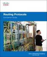
3. Build the topology table. As shown in Figure 6-1, after LSAs are received, OSPF-enabled routers build the topology table (LSDB) based on the received LSAs. This database eventually holds all the information about the topology of the network.
4. Execute the SPF algorithm. Routers then execute the SPF algorithm. The gears in Figure 6-1 are used to indicate the execution of the SPF algorithm. The SPF algorithm creates the SPF tree shown in the figure.
The content of the R1 SPF tree is displayed in Figure 6-2.

From the SPF tree, the best paths are inserted into the routing table. Routing decisions are made based on the entries in the routing table.
Single-Area and Multiarea OSPF (6.1.1.5)
To make OSPF more efficient and scalable, OSPF supports hierarchical routing using areas. An OSPF area is a group of routers that share the same link-state information in their LSDBs.
OSPF can be implemented in one of two ways:
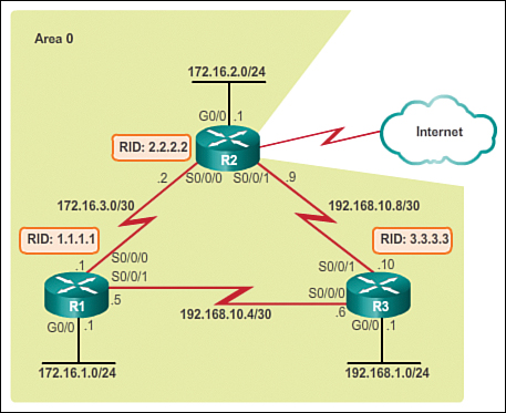
![]() Single-area OSPF: In Figure 6-3, all routers are in one area called the backbone area (area 0). Single-area OSPF is useful in smaller networks with fewer routers.
Single-area OSPF: In Figure 6-3, all routers are in one area called the backbone area (area 0). Single-area OSPF is useful in smaller networks with fewer routers.

![]() Multiarea OSPF: In Figure 6-4, OSPF is implemented using a two-layer area hierarchy as all areas must connect to the backbone area (area 0). A router that interconnects two different areas is referred to as an Area Border Router (ABR). Multiarea OSPF is useful in large network deployments to reduce processing and memory overload.
Multiarea OSPF: In Figure 6-4, OSPF is implemented using a two-layer area hierarchy as all areas must connect to the backbone area (area 0). A router that interconnects two different areas is referred to as an Area Border Router (ABR). Multiarea OSPF is useful in large network deployments to reduce processing and memory overload.

With multiarea OSPF, OSPF can divide one large autonomous system (AS) into smaller areas, to support hierarchical routing. With hierarchical routing, routing still occurs between the areas (inter-area routing), while many of the processor-intensive routing operations, such as recalculating the database, are kept within an area.
For instance, any time a router receives new information about a topology change within the area (including the addition, deletion, or modification of a link), the router must rerun the SPF algorithm, create a new SPF tree, and update the routing table. The SPF algorithm is CPU-intensive and the time it takes for calculation depends on the size of the area.
Note
Topology changes are distributed to routers in other areas in a distance vector format. In other words, these routers only update their routing tables and do not need to rerun the SPF algorithm.
Too many routers in one area would make the LSDBs very large and increase the load on the CPU. Therefore, arranging routers into areas effectively partitions a potentially large database into smaller and more manageable databases.
The hierarchical-topology possibilities of multiarea OSPF have these advantages:
![]() Smaller routing tables: Fewer routing table entries because network addresses can be summarized between areas. Route summarization is not enabled by default.
Smaller routing tables: Fewer routing table entries because network addresses can be summarized between areas. Route summarization is not enabled by default.
![]() Reduced link-state update overhead: Minimizes processing and memory requirements.
Reduced link-state update overhead: Minimizes processing and memory requirements.
![]() Reduced frequency of SPF calculations: Localizes the impact of a topology change within an area. For instance, it minimizes routing update impact because LSA flooding stops at the area boundary as shown in Figure 6-5.
Reduced frequency of SPF calculations: Localizes the impact of a topology change within an area. For instance, it minimizes routing update impact because LSA flooding stops at the area boundary as shown in Figure 6-5.

For example, in Figure 6-5, R2 is an ABR for area 51. As an ABR, it would summarize the area 51 routes into area 0. When one of the summarized links fails, LSAs are exchanged within area 51 only. Routers in area 51 must rerun the SPF algorithm to identify the best routes. However, the routers in area 0 and area 1 do not receive any updates; therefore, they do not execute the SPF algorithm.
The focus of this chapter is on single-area OSPF.
![]() Activity 6.1.1.6: Identify OSPF Features and Terminology
Activity 6.1.1.6: Identify OSPF Features and Terminology
Go to the online course to perform this practice activity.
OSPF Messages (6.1.2)
There are five types of OSPF messages that OSPF-enabled routers use to achieve convergence. This section describes the contents of these encapsulated OSPF messages and the five packet types.
Encapsulating OSPF Messages (6.1.2.1)
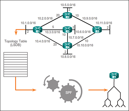
OSPF messages transmitted over an Ethernet link contain the following information:
![]() Data Link Ethernet Frame Header: Identifies the destination multicast MAC address 01-00-5E-00-00-05 or 01-00-5E-00-00-06.
Data Link Ethernet Frame Header: Identifies the destination multicast MAC address 01-00-5E-00-00-05 or 01-00-5E-00-00-06.
![]() IP Packet Header: Identifies the IPv4 protocol field 89, which indicates that this is an OSPF packet. It also identifies one of two OSPF multicast addresses, 224.0.0.5 or 224.0.0.6.
IP Packet Header: Identifies the IPv4 protocol field 89, which indicates that this is an OSPF packet. It also identifies one of two OSPF multicast addresses, 224.0.0.5 or 224.0.0.6.
![]() OSPF Packet Header: Identifies the OSPF packet type, the router ID, and the area ID.
OSPF Packet Header: Identifies the OSPF packet type, the router ID, and the area ID.
![]() OSPF Packet Type–Specific Data: Contains the OSPF packet type information. The content differs depending on the packet type. In this case, it is an IPv4 Header.
OSPF Packet Type–Specific Data: Contains the OSPF packet type information. The content differs depending on the packet type. In this case, it is an IPv4 Header.
Figure 6-6 displays the OSPFv2 field headers and summarizes the content of each header.

Types of OSPF Packets (6.1.2.2)
![]()
Some OSPF Terminology
OSPF uses link-state packets (LSPs) to establish and maintain neighbor adjacencies and exchange routing updates.
There are five different types of LSPs used by OSPF. Each packet serves a specific purpose in the OSPF routing process:
![]() Type 1: Hello packet: Used to discover, establish, and maintain adjacency with other OSPF routers.
Type 1: Hello packet: Used to discover, establish, and maintain adjacency with other OSPF routers.
![]() Type 2: Database Description (DBD) packet: Contains an abbreviated list of the sending router’s LSDB and is used by receiving routers to check against the local LSDB. The LSDB must be identical on all link-state routers within an area to construct an accurate SPF tree.
Type 2: Database Description (DBD) packet: Contains an abbreviated list of the sending router’s LSDB and is used by receiving routers to check against the local LSDB. The LSDB must be identical on all link-state routers within an area to construct an accurate SPF tree.
![]() Type 3: Link-State Request (LSR) packet: Receiving routers can then request more information about any entry in the DBD by sending an LSR.
Type 3: Link-State Request (LSR) packet: Receiving routers can then request more information about any entry in the DBD by sending an LSR.
![]() Type 4: Link-State Update (LSU) packet: Used to reply to LSRs and to announce new information. LSUs contain seven different types of LSAs.
Type 4: Link-State Update (LSU) packet: Used to reply to LSRs and to announce new information. LSUs contain seven different types of LSAs.
![]() Type 5: Link-State Acknowledgment (LSAck) packet: When an LSU is received, the router sends an LSAck to confirm receipt of the LSU. The LSAck data field is empty.
Type 5: Link-State Acknowledgment (LSAck) packet: When an LSU is received, the router sends an LSAck to confirm receipt of the LSU. The LSAck data field is empty.
Hello Packet (6.1.2.3)
![]()
Neighborship vs. Adjacency
The OSPF Type 1 packet is the Hello packet. Hello packets are used to:
![]() Discover OSPF neighbors and establish neighbor adjacencies.
Discover OSPF neighbors and establish neighbor adjacencies.
![]() Advertise parameters on which two routers must agree to become neighbors.
Advertise parameters on which two routers must agree to become neighbors.
![]() Elect the Designated Router (DR) and Backup Designated Router (BDR) on multi-access networks like Ethernet and Frame Relay. Point-to-point links do not require DR or BDR.
Elect the Designated Router (DR) and Backup Designated Router (BDR) on multi-access networks like Ethernet and Frame Relay. Point-to-point links do not require DR or BDR.
Figure 6-7 displays the fields contained in the Type 1 Hello packet.
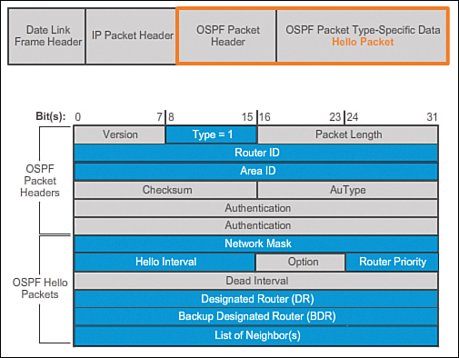
Important fields shown in the figure include:
![]() Type: Identifies the type of packet. A one (1) indicates a Hello packet. A value of 2 identifies a DBD packet, 3 an LSR packet, 4 an LSU packet, and 5 an LSAck packet.
Type: Identifies the type of packet. A one (1) indicates a Hello packet. A value of 2 identifies a DBD packet, 3 an LSR packet, 4 an LSU packet, and 5 an LSAck packet.
![]() Router ID: A 32-bit value expressed in dotted-decimal notation (an IPv4 address) used to uniquely identify the originating router.
Router ID: A 32-bit value expressed in dotted-decimal notation (an IPv4 address) used to uniquely identify the originating router.
![]() Area ID: Area from which the packet originated.
Area ID: Area from which the packet originated.
![]() Network Mask: Subnet mask associated with the sending interface.
Network Mask: Subnet mask associated with the sending interface.
![]() Hello Interval: Specifies the frequency, in seconds, at which a router sends Hello packets. The default Hello interval on multi-access and point-to-point networks is 10 seconds. This timer must be the same on neighboring routers; otherwise, an adjacency is not established.
Hello Interval: Specifies the frequency, in seconds, at which a router sends Hello packets. The default Hello interval on multi-access and point-to-point networks is 10 seconds. This timer must be the same on neighboring routers; otherwise, an adjacency is not established.
![]() Router Priority: Used in a DR/BDR election. The default priority for all OSPF routers is 1, but can be manually altered from 0 to 255. The higher the value, the more likely the router becomes the DR on the link.
Router Priority: Used in a DR/BDR election. The default priority for all OSPF routers is 1, but can be manually altered from 0 to 255. The higher the value, the more likely the router becomes the DR on the link.
![]() Dead Interval: Is the time, in seconds, that a router waits to hear from a neighbor before declaring the neighboring router out of service. By default, the router Dead Interval is four times the Hello interval. This timer must be the same on neighboring routers; otherwise, an adjacency is not established.
Dead Interval: Is the time, in seconds, that a router waits to hear from a neighbor before declaring the neighboring router out of service. By default, the router Dead Interval is four times the Hello interval. This timer must be the same on neighboring routers; otherwise, an adjacency is not established.
![]() Designated Router (DR): Router ID of the DR.
Designated Router (DR): Router ID of the DR.
![]() Backup Designated Router (BDR): Router ID of the BDR.
Backup Designated Router (BDR): Router ID of the BDR.
![]() List of Neighbors: List that identifies the router IDs of all adjacent routers.
List of Neighbors: List that identifies the router IDs of all adjacent routers.
Hello Packet Intervals (6.1.2.4)
OSPF Hello packets are transmitted to multicast address 224.0.0.5 in IPv4 and FF02::5 in IPv6 (all OSPF routers) every:
![]() 10 seconds (default on multi-access and point-to-point networks)
10 seconds (default on multi-access and point-to-point networks)
![]() 30 seconds (default on nonbroadcast multi-access [NBMA] networks; for example, Frame Relay)
30 seconds (default on nonbroadcast multi-access [NBMA] networks; for example, Frame Relay)
The Dead Interval is the period that the router waits to receive a Hello packet before declaring the neighbor down. If the Dead Interval expires before the routers receive a Hello packet, OSPF removes that neighbor from its LSDB. The router floods the LSDB with information about the down neighbor out all OSPF-enabled interfaces.
Cisco uses a default of four times the Hello interval:
![]() 40 seconds (default on multi-access and point-to-point networks)
40 seconds (default on multi-access and point-to-point networks)
![]() 120 seconds (default on NBMA networks; for example, Frame Relay)
120 seconds (default on NBMA networks; for example, Frame Relay)
Link-State Updates (6.1.2.5)
Routers initially exchange Type 2 DBD packets, which is an abbreviated list of the sending router’s LSDB and is used by receiving routers to check against the local LSDB.
A Type 3 LSR packet is used by the receiving routers to request more information about an entry in the DBD.
The Type 4 LSU packet is used to reply to an LSR packet.
LSUs are also used to forward OSPF routing updates, such as link changes. Specifically, an LSU packet can contain 11 different types of OSPFv2 LSAs, as shown in Figure 6-8. OSPFv3 renamed several of these LSAs and also contains two additional LSAs.

Note
The difference between the LSU and LSA terms can sometimes be confusing because these terms are often used interchangeably. However, an LSU contains one or more LSAs.
![]() Activity 6.1.2.6: Identify the OSPF Packet Types
Activity 6.1.2.6: Identify the OSPF Packet Types
Go to the online course to perform this practice activity.
OSPF Operation (6.1.3)
![]()
Lesson 1: Review of OSPF Operation
OSPF routers must first become neighbors, exchange routing information, and achieve convergence. This section describes how OSPF neighbors transition between several states to achieve this convergence.
OSPF Operational States (6.1.3.1)
When an OSPF router is initially connected to a network, it attempts to:
![]() Create adjacencies with neighbors
Create adjacencies with neighbors
![]() Exchange routing information
Exchange routing information
![]() Calculate the best routes
Calculate the best routes
![]() Reach convergence
Reach convergence
OSPF progresses through several states while attempting to reach convergence. The first three states are used to establish neighbor adjacencies:
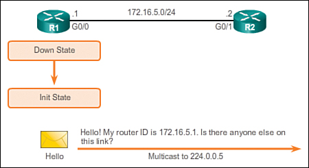
![]() Down state: This is when there are no Hello packets exchanged. When a router sends and receives Hello packets, OSPF transitions to the Init state.
Down state: This is when there are no Hello packets exchanged. When a router sends and receives Hello packets, OSPF transitions to the Init state.
![]() Init state: This state starts when a router receives a Hello packet that contains the sender’s router ID.
Init state: This state starts when a router receives a Hello packet that contains the sender’s router ID.
![]() Two-Way state: On Ethernet links, routers elect a Designated Router (DR) and Backup Designated Router (BDR).
Two-Way state: On Ethernet links, routers elect a Designated Router (DR) and Backup Designated Router (BDR).
Once adjacencies are established, the routers proceed to the following states to synchronize their OSPF databases:
![]() ExStart state: Routers negotiate a master/slave relationship and the master initiates the DBD exchange.
ExStart state: Routers negotiate a master/slave relationship and the master initiates the DBD exchange.
![]() Exchange state: Each router forwards its DBD.
Exchange state: Each router forwards its DBD.
![]() Loading state: If additional information is required, the routers use LSRs and LSUs to gain additional router information. Routers are processed using the SPF algorithm.
Loading state: If additional information is required, the routers use LSRs and LSUs to gain additional router information. Routers are processed using the SPF algorithm.
![]() Full state: This state is achieved only when the routers have converged.
Full state: This state is achieved only when the routers have converged.
Establish Neighbor Adjacencies (6.1.3.2)
![]()
Forming an Adjacency
![]()
Configuring Neighbor Authentication
When OSPF is enabled on an interface, the router must determine if there is another OSPF neighbor on the link. To accomplish this, the router forwards a Hello packet that contains its router ID out all OSPF-enabled interfaces. The OSPF router ID is used by the OSPF process to uniquely identify each router in the OSPF area. A router ID is an IP address assigned to identify a specific router among OSPF peers.
When a neighboring OSPF-enabled router receives a Hello packet with a router ID that is not within its neighbor list, the receiving router attempts to establish an adjacency with the initiating router.
Refer to R1 in Figure 6-9. When OSPF is enabled, the enabled GigabitEthernet 0/0 interface transitions from the Down state to the Init state. R1 starts sending Hello packets out all OSPF-enabled interfaces to discover OSPF neighbors to develop adjacencies with.
In Figure 6-10, R2 receives the Hello packet from R1 and adds the R1 router ID to its neighbor list. R2 then sends a Hello packet to R1. The packet contains the R2 router ID and the R1 router ID in its list of neighbors on the same interface.

When R1 receives the Hello, it adds the R2 router ID to its list of OSPF neighbors. It also notices its own router ID in the Hello packet’s list of neighbors. When a router receives a Hello packet with its router ID listed in the list of neighbors, the router transitions from the Init state to the Two-Way state.
The action performed in Two-Way state depends on the type of inter-connection between the adjacent routers:
![]() If the two adjacent neighbors are interconnected over a point-to-point link, then they immediately transition from the Two-Way state to the database synchronization phase.
If the two adjacent neighbors are interconnected over a point-to-point link, then they immediately transition from the Two-Way state to the database synchronization phase.
![]() If the routers are interconnected over a common Ethernet network, then a Designated Router DR and a BDR must be elected.
If the routers are interconnected over a common Ethernet network, then a Designated Router DR and a BDR must be elected.
Because R1 and R2 are interconnected over an Ethernet network, a DR and BDR election takes place. As shown in Figure 6-11, R2 becomes the DR and R1 is the BDR. This process only occurs on multiaccess networks such as Ethernet LANs.

Note
Hello packets will continue to be exchanged to maintain neighbor adjacencies.
OSPF DR and BDR (6.1.3.3)
![]()
Influencing Designated Router Selection
Why is a DR and BDR election necessary?
Multi-access networks can create two challenges for OSPF regarding the flooding of LSAs:
![]() Creation of multiple adjacencies: Ethernet networks could potentially interconnect many OSPF routers over a common link. Creating adjacencies with every router is unnecessary and undesirable. It would lead to an excessive number of LSAs exchanged between routers on the same network.
Creation of multiple adjacencies: Ethernet networks could potentially interconnect many OSPF routers over a common link. Creating adjacencies with every router is unnecessary and undesirable. It would lead to an excessive number of LSAs exchanged between routers on the same network.
![]() Extensive flooding of LSAs: Link-state routers flood their LSAs any time OSPF is initialized, or when there is a change in the topology. This flooding can become excessive.
Extensive flooding of LSAs: Link-state routers flood their LSAs any time OSPF is initialized, or when there is a change in the topology. This flooding can become excessive.
To understand the problem with multiple adjacencies, we must study a formula.
For any number of routers (designated as n) on a multi-access network, there are n (n – 1) / 2 adjacencies.
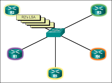
Figure 6-12 shows a simple topology of five routers, all of which are attached to the same multi-access Ethernet network.

Without some type of mechanism to reduce the number of adjacencies, collectively these routers would form 10 adjacencies:
5 (5 – 1) / 2 = 10
This may not seem like much, but as routers are added to the network, the number of adjacencies increases dramatically, as shown in Table 6-4.

To understand the problem of extensive flooding of LSAs, refer to Figure 6-13. In the example, R2 is advertising a new route and therefore sends individual LSAs to each of its OSPF neighbors.
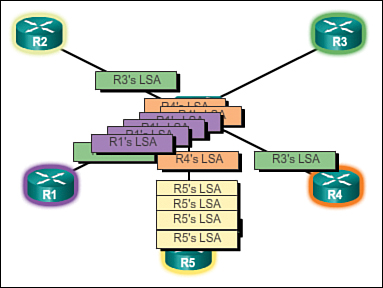
This event triggers every neighbor router to also send out an LSA, as illustrated in Figure 6-14. Not shown in the figure are the required acknowledgments sent for every LSA received. If every router in a multi-access network had to flood and acknowledge all received LSAs to all other routers on that same multi-access network, the network traffic would become quite chaotic.
![]() Video 6.1.3.3-A: Flooding LSAs
Video 6.1.3.3-A: Flooding LSAs
Go to the online course and play the animation in the third graphic to see how exchanging LSAs without a DR generates a flood of LSAs to be exchanged.
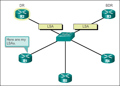
The solution to managing the number of adjacencies and the flooding of LSAs on a multi-access network is the DR. On multi-access networks, OSPF elects a DR to be the collection and distribution point for LSAs sent and received. A BDR is also elected in case the DR fails. All other routers become DROTHERs. A DROTHER is a router that is neither the DR nor the BDR.
In Figure 6-15, R2 has been elected the DR and R3 is the BDR. When a route change occurs on R1, it sends an LSA to the DR and BDR only using the multicast address of 224.0.0.6 (All Designated Routers).
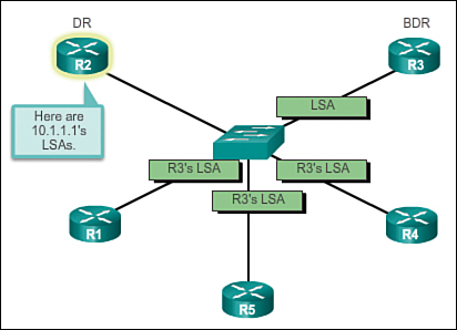
As shown in Figure 6-16, the DR then sends LSAs to all of its OSPF adjacencies on behalf of R1 using the multicast address of 224.0.0.5 (All OSPF Routers).
Go to the online course and play the animation in the fourth graphic to see how the number of LSAs is reduced when using the services of a DR.
Synchronizing OSPF Databases (6.1.3.4)
After the Two-Way state, routers transition to database synchronization states. While the Hello packet was used to establish neighbor adjacencies, the other four types of OSPF packets are used during the process of exchanging and synchronizing LSDBs.
In the ExStart state, a master and slave relationship is created between each router and its adjacent DR and BDR. The router with the higher router ID acts as the master for the Exchange state. In Figure 6-17, R2 becomes the master.

In the Exchange state, the master and slave routers exchange one or more DBD packets. A DBD packet includes information about the LSA entry header that appears in the router’s LSDB. The entries can be about a link or about a network. Each LSA entry header includes information about the link-state type, the address of the advertising router, the link’s cost, and the sequence number. The router uses the sequence number to determine the newness of the received link-state information.
In Figure 6-18, R2 sends a DBD packet to R1.

When R1 receives the DBD packet, the following actions occur:
1. R1 acknowledges the receipt of the DBD using the LSAck packet.
2. R1 then sends DBD packets to R2.
3. R2 acknowledges R1.
R1 compares the information received with the information it has in its own LSDB. If the DBD packet has a more current link-state entry, the router transitions to the Loading state.
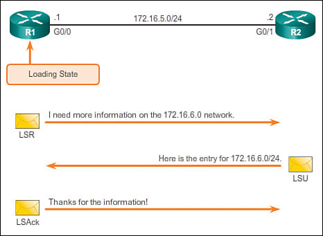
For example, in Figure 6-19, R1 sends an LSR regarding network 172.16.6.0 to R2. R2 responds with the complete information about 172.16.6.0 in an LSU packet. Again, when R1 receives an LSU, it sends an LSAck. R1 then adds the new link-state entries into its LSDB.
After all LSRs have been satisfied for a given router, the adjacent routers are considered synchronized and in a Full state.
As long as the neighboring routers continue receiving Hello packets, the network in the transmitted LSAs remain in the topology database. After the topological databases are synchronized, updates (LSUs) are sent only to neighbors when:
![]() A change is perceived (incremental updates)
A change is perceived (incremental updates)
![]() Every 30 minutes
Every 30 minutes
![]() Activity 6.1.3.5: Identify the OSPF States for Establishing Adjacency
Activity 6.1.3.5: Identify the OSPF States for Establishing Adjacency
Go to the online course to perform this practice activity.
![]() Video 6.1.3.6: Observing OSPF Protocol Communications
Video 6.1.3.6: Observing OSPF Protocol Communications
Go to the online course and play the animation to see how to configure OSPFv2 and then observe the neighbor adjacencies.
Configuring Single-Area OSPFv2 (6.2)
![]()
Lesson 2: OSPFv2 Configuration
This section discusses the commands used for basic OSPF configuration. As you will see, the commands used are not much different from the commands you have already used in other routing protocols.
OSPF Network Topology (6.2.1.1)
Figure 6-20 shows the topology used for configuring OSPFv2 in this section. The types of serial interfaces and their associated bandwidths may not necessarily reflect the more common types of connections found in networks today. The bandwidths of the serial links used in this topology were chosen to help explain the calculation of the routing protocol metrics and the process of best path selection.

The routers in the topology have a starting configuration, including interface addresses. There is currently no static routing or dynamic routing configured on any of the routers. All interfaces on routers R1, R2, and R3 (except the loopback on R2) are within the OSPF backbone area. The loopback interface on R2 is used as the routing domain’s gateway to the Internet.
Note
In this topology the loopback interface is used to simulate the WAN link to the Internet.
Router OSPF Configuration Mode (6.2.1.2)
OSPFv2 is enabled using the router ospf process-id global configuration mode command. The process-id value represents a number between 1 and 65,535 and is selected by the network administrator. The process-id value is locally significant, which means that it does not have to be the same value on the other OSPF routers to establish adjacencies with those neighbors.
Figure 6-21 provides an example of entering router OSPF configuration mode on R1 and displaying some of the OSPF router commands.
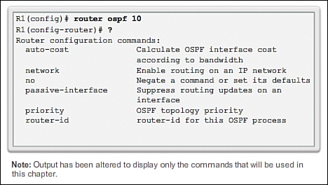
Note
The list of commands has been altered to display only the commands that are used in this chapter.
![]() Activity 6.2.1.2: Entering Router OSPF Configuration Mode on R2
Activity 6.2.1.2: Entering Router OSPF Configuration Mode on R2
Go to the online course to use the Syntax Checker in the third graphic to enter OSPF router configuration mode on R2 and list the commands available at the prompt.
Router IDs (6.2.1.3)
Every router requires a router ID to participate in an OSPF domain. The router ID can be defined by an administrator or automatically assigned by the router. The router ID is used by the OSPF-enabled router to:
![]() Uniquely identify the router: The router ID is used by other routers to uniquely identify each router within the OSPF domain and all packets that originate from them.
Uniquely identify the router: The router ID is used by other routers to uniquely identify each router within the OSPF domain and all packets that originate from them.
![]() Participate in the election of the DR: In a multi-access LAN environment, the election of the DR occurs during initial establishment of the OSPF network. When OSPF links become active, the routing device configured with the highest priority is elected the DR. Assuming there is no priority configured, or there is a tie, then the router with the highest router ID is elected the DR. The routing device with the second highest router ID is elected the BDR.
Participate in the election of the DR: In a multi-access LAN environment, the election of the DR occurs during initial establishment of the OSPF network. When OSPF links become active, the routing device configured with the highest priority is elected the DR. Assuming there is no priority configured, or there is a tie, then the router with the highest router ID is elected the DR. The routing device with the second highest router ID is elected the BDR.
But how does the router determine the router ID? As illustrated in Figure 6-22, Cisco routers derive the router ID based on one of three criteria, in the following preferential order:

![]() The router ID is explicitly configured using the OSPF router-id rid router configuration mode command. The rid value is any 32-bit value expressed as an IPv4 address. This is the recommended method to assign a router ID.
The router ID is explicitly configured using the OSPF router-id rid router configuration mode command. The rid value is any 32-bit value expressed as an IPv4 address. This is the recommended method to assign a router ID.
![]() If the router ID is not explicitly configured, the router chooses the highest IPv4 address of any of the configured loopback interfaces. This is the next best alternative to assigning a router ID.
If the router ID is not explicitly configured, the router chooses the highest IPv4 address of any of the configured loopback interfaces. This is the next best alternative to assigning a router ID.
![]() If no loopback interfaces are configured, then the router chooses the highest active IPv4 address of any of its physical interfaces. This is the least recommended method because it makes it more difficult for administrators to distinguish between specific routers.
If no loopback interfaces are configured, then the router chooses the highest active IPv4 address of any of its physical interfaces. This is the least recommended method because it makes it more difficult for administrators to distinguish between specific routers.
If the router uses the highest IPv4 address for the router ID, the interface does not need to be OSPF-enabled. This means that the interface address does not need to be included in one of the OSPF network commands for the router to use that IP address as the router ID. The only requirement is that the interface is active and in the up state.
Note
The router ID looks like an IP address, but it is not routable and, therefore, is not included in the routing table, unless the OSPF routing process chooses an interface (physical or loopback) that is appropriately defined by a network command.
Configuring an OSPF Router ID (6.2.1.4)
Use the router-id rid router configuration mode command to manually assign a 32-bit value expressed as an IPv4 address to a router. An OSPF router identifies itself to other routers using this router ID.
As shown in Figure 6-23, R1 should be assigned the router ID of 1.1.1.1, R2 the router ID of 2.2.2.2, and R3 the router ID of 3.3.3.3.
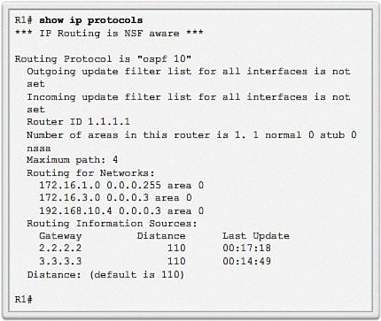
In Figure 6-24, the router ID 1.1.1.1 is assigned to R1. Use the show ip protocols command to verify the router ID.

Note
R1 had never been configured with an OSPF router ID. If it had, then the router ID would have to be modified.
If the router ID is the same on two neighboring routers, the router displays an error message similar to the one below:
%OSPF-4-DUP_RTRID1: Detected router with duplicate router ID.
To correct this problem, configure all routers so that they have unique OSPF router IDs.
![]() Activity 6.2.1.4: Assigning the Router ID on R2 and R3
Activity 6.2.1.4: Assigning the Router ID on R2 and R3
Go to the online course to use the Syntax Checker in the third graphic to assign the router ID on R2 and R3.
Modifying a Router ID (6.2.1.5)
Sometimes a router ID needs to be changed, for example, when a network administrator establishes a new router ID scheme for the network. However, after a router selects a router ID, an active OSPF router does not allow the router ID to be changed until the router is reloaded or the OSPF process is cleared.
In Figure 6-25, notice that the current router ID is 192.168.10.5. The router ID should be 1.1.1.1.

In the following listing, the router ID 1.1.1.1 is being assigned to R1. Notice in the output how an informational message appears stating that the OSPF process must be cleared or that the router must be reloaded. The reason is because R1 already has adjacencies with other neighbors using the router ID 192.168.10.5. Those adjacencies must be renegotiated using the new router IP 1.1.1.1.
R1(config)# router ospf 10
R1(config-router)# router-id 1.1.1.1
% OSPF: Reload or use "clear ip ospf process" command, for this to take effect
R1(config-router)# end
R1#
*Mar 25 19:46:09.711: %SYS-5-CONFIG_I: Configured from console by console
Clearing the OSPF process is the preferred method to reset the router ID.
In Figure 6-26, the OSPF routing process is cleared using the clear ip ospf process privileged EXEC mode command. This forces OSPF on R1 to transition to the Down and Init states. Notice the adjacency messages change from Full to Down and then from Loading to Full. The show ip protocols command verifies that the router ID has changed.

![]() Activity 6.2.1.5: Modifying the Router ID
Activity 6.2.1.5: Modifying the Router ID
Go to the online course to use the Syntax Checker in the fourth graphic to modify the router ID for R1.
Using a Loopback Interface as the Router ID (6.2.1.6)
A router ID can also be assigned using a loopback interface.
The IPv4 address of the loopback interface should be configured using a 32-bit subnet mask (255.255.255.255). This effectively creates a host route. A 32-bit host route does not get advertised as a route to other OSPF routers.
The following displays how to configure a loopback interface with a host route on R1. R1 uses the host route as its router ID, assuming there is no router ID explicitly configured or previously learned.
R1(config)# interface loopback 0
R1(config-if)# ip address 1.1.1.1 255.255.255.255
R1(config-if)# end
R1#
Note
Some older versions of the IOS do not recognize the router-id command; therefore, the best way to set the router ID on those routers is by using a loopback interface.
Configure Single-Area OSPFv2 (6.2.2)
![]()
Single-Area OSPF
![]()
Benefits
![]()
OSPFv2 Configuration and Verification
This section discusses the commands used for configuring basic single-area OSPFv2.
Enabling OSPF on Interfaces (6.2.2.1)
The network command determines which interfaces participate in the routing process for an OSPF area. Any interfaces on a router that match the network address in the network command are enabled to send and receive OSPF packets. As a result, the network (or subnet) address for the interface is included in OSPF routing updates.
The basic command syntax is network network-address wildcard-mask area area-id.
The area area-id syntax refers to the OSPF area. When configuring single-area OSPF, the network command must be configured with the same area-id value on all routers. Although any area ID can be used, it is good practice to use an area ID of 0 with single-area OSPF. This convention makes it easier if the network is later altered to support multiarea OSPF.
Wildcard Mask (6.2.2.2)
OSPFv2 uses the argument combination of network-address wildcard-mask to enable OSPF on interfaces. OSPF is classless by design; therefore, the wildcard mask is always required. When identifying interfaces that are participating in a routing process, the wildcard mask is typically the inverse of the subnet mask configured on that interface.
A wildcard mask is a string of 32 binary digits used by the router to determine which bits of the address to examine for a match. In a subnet mask, binary 1 is equal to a match and binary 0 is not a match. In a wildcard mask, the reverse is true:
![]() Wildcard mask bit 0: Matches the corresponding bit value in the address
Wildcard mask bit 0: Matches the corresponding bit value in the address
![]() Wildcard mask bit 1: Ignores the corresponding bit value in the address
Wildcard mask bit 1: Ignores the corresponding bit value in the address
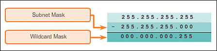
The easiest method for calculating a wildcard mask is to subtract the network subnet mask from 255.255.255.255.
The example in Figure 6-27 calculates the wildcard mask from the network address of 192.168.10.0/24. To do so, the subnet mask 255.255.255.0 is subtracted from 255.255.255.255, providing a result of 0.0.0.255. Therefore, 192.168.10.0/24 is 192.168.10.0 with a wildcard mask of 0.0.0.255.
The example in Figure 6-28 calculates the wildcard mask from the network address of 192.168.10.64/26. Again, the subnet mask 255.255.255.192 is subtracted from 255.255.255.255, providing a result of 0.0.0.63. Therefore, 192.168.10.0/26 is 192.168.10.0 with a wildcard mask of 0.0.0.63.

The network Command (6.2.2.3)
There are several ways to identify the interfaces that will participate in the OSPFv2 routing process.
The following displays the required commands to determine which interfaces on R1 participate in the OSPFv2 routing process for an area. Notice the use of wildcard masks to identify the respective interfaces based on their network addresses. Because this is a single-area OSPF network, all area IDs are set to 0.
R1(config)# router ospf 10
R1(config-router)# network 172.16.1.0 0.0.0.255 area 0
R1(config-router)# network 172.16.3.0 0.0.0.3 area 0
R1(config-router)# network 192.168.10.4 0.0.0.3 area 0
R1(config-router)#
As an alternative, OSPFv2 can be enabled using the network intf-ip-address 0.0.0.0 area area-id router configuration mode command.
The following is an example of specifying the interface IPv4 address with a quad 0 wildcard mask. Entering network 172.16.3.1 0.0.0.0 area 0 on R1 tells the router to enable interface Serial l0/0/0 for the routing process. As a result, the OSPFv2 process will advertise the network that is on this interface (172.16.3.0/30).
R1(config)# router ospf 10
R1(config-router)# network 172.16.1.1 0.0.0.0 area 0
R1(config-router)# network 172.16.3.1 0.0.0.0 area 0
R1(config-router)# network 192.168.10.5 0.0.0.0 area 0
R1(config-router)#
The advantage of specifying the interface is that the wildcard mask calculation is not necessary. OSPFv2 uses the interface address and subnet mask to determine the network to advertise.
Some IOS versions allow the subnet mask to be entered instead of the wildcard mask. The IOS then converts the subnet mask to the wildcard mask format.
![]() Activity 6.2.2.3: Advertising Networks in OSPF
Activity 6.2.2.3: Advertising Networks in OSPF
Go to the online course to use the Syntax Checker in the third graphic to advertise the networks connected to R2.
Note
While completing the Syntax Checker, observe the informational messages describing the adjacency between R1 (1.1.1.1) and R2 (2.2.2.2). The IPv4 addressing scheme used for the router ID makes it easy to identify the neighbor.
Passive Interface (6.2.2.4)
By default, OSPF messages are forwarded out all OSPF-enabled interfaces. However, these messages really only need to be sent out interfaces connecting to other OSPF-enabled routers.
Refer to the topology in Figure 6-23. OSPF messages are forwarded out of all three routers’ G0/0 interface even though no OSPF neighbor exists on that LAN. Sending out unneeded messages on a LAN affects the network in three ways:
![]() Inefficient use of bandwidth: Available bandwidth is consumed transporting unnecessary messages. Messages are multicasted; therefore, switches are also forwarding the messages out all ports.
Inefficient use of bandwidth: Available bandwidth is consumed transporting unnecessary messages. Messages are multicasted; therefore, switches are also forwarding the messages out all ports.
![]() Inefficient use of resources: All devices on the LAN must process the message and eventually discard the message.
Inefficient use of resources: All devices on the LAN must process the message and eventually discard the message.
![]() Increased security risk: Advertising updates on a broadcast network is a security risk. OSPF messages can be intercepted with packet sniffing software. Routing updates can be modified and sent back to the router, corrupting the routing table with false metrics that misdirect traffic.
Increased security risk: Advertising updates on a broadcast network is a security risk. OSPF messages can be intercepted with packet sniffing software. Routing updates can be modified and sent back to the router, corrupting the routing table with false metrics that misdirect traffic.
Configuring Passive Interfaces (6.2.2.5)
Use the passive-interface router configuration mode command to prevent the transmission of routing messages through a router interface but still allow that network to be advertised to other routers, as shown next for router R1. Specifically, the command stops routing messages from being sent out the specified interface. However, the network that the specified interface belongs to is still advertised in routing messages that are sent out other interfaces.
R1(config)# router ospf 10
R1(config-router)# passive-interface GigabitEthernet 0/0
R1(config-router)# end
R1#
For instance, there is no need for R1, R2, and R3 to forward OSPF messages out of their LAN interfaces. The configuration identifies the R1 G0/0 interface as passive.
It is important to know that a neighbor adjacency cannot be formed over a passive interface. This is because link-state packets cannot be sent or acknowledged.
The show ip protocols command is then used to verify that the Gigabit Ethernet interface was passive, as shown in Figure 6-29. Notice that the G0/0 interface is now listed under the Passive Interface(s) section. The network 172.16.1.0 is still listed under Routing for Networks, which means that this network is still included as a route entry in OSPF updates that are sent to R2 and R3.

Note
OSPFv2 and OSPFv3 both support the passive-interface command.
As an alternative, all interfaces can be made passive using the passive-interface default command. Interfaces that should not be passive can be re-enabled using the no passive-interface command.
![]() Activity 6.2.2.5: Configuring Passive Interfaces
Activity 6.2.2.5: Configuring Passive Interfaces
Go to the online course to use the Syntax Checker in the third graphic to configure the LAN interfaces as passive interfaces on R2 and R3.
Note
While completing the Syntax Checker, notice the OSPF informational state messages as the interfaces are all rendered passive and then the two serial interfaces are made non-passive.
![]() Activity 6.2.2.6: Calculate the Subnet and Wildcard Masks
Activity 6.2.2.6: Calculate the Subnet and Wildcard Masks
Go to the online course to perform this practice activity.
![]() Packet Tracer Activity 6.2.2.7: Configuring OSPFv2 in a Single-Area
Packet Tracer Activity 6.2.2.7: Configuring OSPFv2 in a Single-Area
In this activity, the IP addressing is already configured. You are responsible for configuring the three-router topology with basic single-area OSPFv2, and then verifying connectivity between end devices.
OSPF Cost (6.2.3)
![]()
Measuring Cost
The OSPF metric is called cost. In this topic you will learn how Cisco IOS Software uses the cumulative bandwidths of the outgoing interfaces from the router to the destination network as the cost value.
OSPF Metric = Cost (6.2.3.1)
Recall that a routing protocol uses a metric to determine the best path of a packet across a network. A metric gives indication of the overhead that is required to send packets across a certain interface. OSPF uses cost as a metric. A lower cost indicates a better path than a higher cost.
The cost of an interface is inversely proportional to the bandwidth of the interface. Therefore, a higher bandwidth indicates a lower cost. More overhead and time delays equal a higher cost. Therefore, a 10-Mb/s Ethernet line has a higher cost than a 100-Mb/s Ethernet line.
The formula used to calculate the OSPF cost is:
Cost = reference bandwidth / interface bandwidth
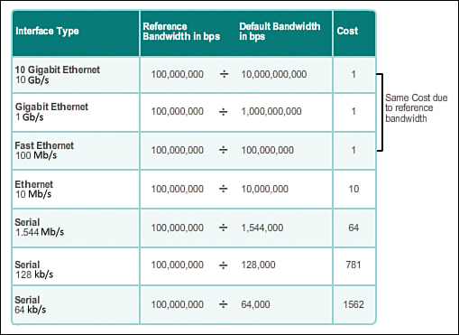
The default reference bandwidth is 10^8 (100,000,000); therefore, the formula is:
Cost = 100,000,000 b/s / interface bandwidth in b/s
Refer to Figure 6-30 for a breakdown of the cost calculation. Notice that Fast Ethernet, Gigabit Ethernet, and 10-Gigabit Ethernet interfaces share the same cost, because the OSPF cost value must be an integer. Consequently, because the default reference bandwidth is set to 100 Mb/s, all links that are faster than Fast Ethernet also have a cost of 1.
OSPF Accumulates Costs (6.2.3.2)
The cost of an OSPF route is the accumulated value from one router to the destination network.
For example, in Figure 6-31, the cost to reach the R2 LAN 172.16.2.0/24 from R1 should be as follows:
![]() Serial link from R1 to R2 cost = 64
Serial link from R1 to R2 cost = 64
![]() Gigabit Ethernet link on R2 cost = 1
Gigabit Ethernet link on R2 cost = 1
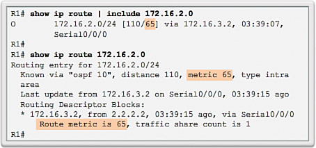
![]() Total cost to reach 172.16.2.0/24 = 65
Total cost to reach 172.16.2.0/24 = 65

The routing table of R1 in Figure 6-32 confirms that the metric to reach the R2 LAN is a cost of 65.
Adjusting the Reference Bandwidth (6.2.3.3)
OSPF uses a reference bandwidth of 100 Mb/s for any links that are equal to or faster than a Fast Ethernet connection. Therefore, the cost assigned to a Fast Ethernet interface with an interface bandwidth of 100 Mb/s would equal 1:
Cost = 100,000,000 b/s / 100,000,000 = 1
While this calculation works for Fast Ethernet interfaces, it is problematic for links that are faster than 100 Mb/s, because the OSPF metric only uses integers as its final cost of a link. If something less than an integer is calculated, OSPF rounds up to the nearest integer. For this reason, from the OSPF perspective, an interface with an interface bandwidth of 100 Mb/s (a cost of 1) has the same cost as an interface with a bandwidth of 100 Gb/s (a cost of 1).
To assist OSPF in making the correct path determination, the reference bandwidth must be changed to a higher value to accommodate networks with links faster than 100 Mb/s.
Adjusting the Reference Bandwidth
Changing the reference bandwidth does not actually affect the bandwidth capacity on the link; rather, it simply affects the calculation used to determine the metric. To adjust the reference bandwidth, use the auto-cost reference-bandwidth Mb/s router configuration command. This command must be configured on every router in the OSPF domain. Notice that the value is expressed in Mb/s; therefore, to adjust the costs for:
![]() Gigabit Ethernet: Use the auto-cost reference-bandwidth 1000 command
Gigabit Ethernet: Use the auto-cost reference-bandwidth 1000 command
![]() 10-Gigabit Ethernet: Use auto-cost reference-bandwidth 10000 command
10-Gigabit Ethernet: Use auto-cost reference-bandwidth 10000 command
To return to the default reference bandwidth, use the auto-cost reference-bandwidth 100 command.
Note
The reference bandwidth should be adjusted any time there are links faster than Fast Ethernet (100 Mb/s).
Table 6-5 displays the OSPF cost if the reference bandwidth is set to Gigabit Ethernet. Although the metric values increase, OSPF makes better choices because it can now distinguish between Fast Ethernet and Gigabit Ethernet links.

Table 6-6 displays the OSPF cost if the reference bandwidth is adjusted to accommodate 10-Gigabit Ethernet links.

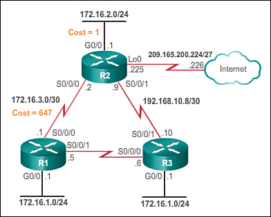
In Figure 6-33, all routers have been configured to accommodate the Gigabit Ethernet link with the auto-cost reference-bandwidth 1000 router configuration command. The following is the new accumulated cost to reach the R2 LAN 172.16.2.0/24 from R1:
![]() Serial link from R1 to R2 cost = 647
Serial link from R1 to R2 cost = 647
![]() Gigabit Ethernet link on R2 cost = 1
Gigabit Ethernet link on R2 cost = 1
![]() Total cost to reach 172.16.2.0/24 = 648
Total cost to reach 172.16.2.0/24 = 648
Use the show ip ospf interface s0/0/0 command to verify the current OSPF cost assigned to the R1 Serial 0/0/0 interface, as shown in Figure 6-34. Notice how it displays a cost of 647.

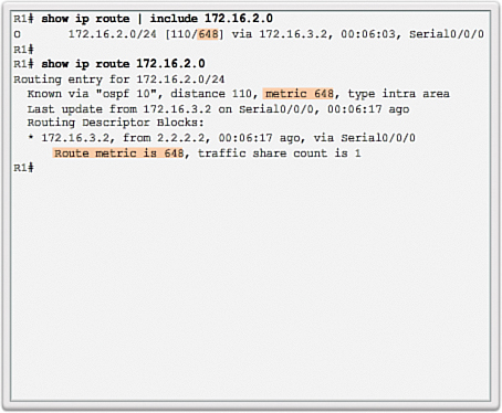
The routing table of R1 in Figure 6-35 confirms that the metric to reach the R2 LAN is a cost of 648.
Default Interface Bandwidths (6.2.3.4)
All interfaces have default bandwidth values assigned to them. As with reference bandwidth, interface bandwidth values do not actually affect the speed or capacity of the link. Instead, they are used by OSPF to compute the routing metric. Therefore, it is important that the bandwidth value reflect the actual speed of the link so that the routing table has accurate best path information.
Although the bandwidth values of Ethernet interfaces usually match the link speed, some other interfaces may not. For instance, the actual speed of serial interfaces is often different than the default bandwidth. On Cisco routers, the default bandwidth on most serial interfaces is set to 1.544 Mb/s.
Note
Older serial interfaces may default to 128 kb/s.
Refer to the example in Figure 6-36. Notice that the link between:
![]() R1 and R2 should be set to 1,544 kb/s (default value)
R1 and R2 should be set to 1,544 kb/s (default value)
![]() R2 and R3 should be set to 1,024 kb/s
R2 and R3 should be set to 1,024 kb/s
![]() R1 and R3 should be set to 64 kb/s
R1 and R3 should be set to 64 kb/s

Use the show interfaces command to view the interface bandwidth setting. Figure 6-37 displays the serial 0/0/0 interface settings for R1. The bandwidth setting is accurate and therefore the serial interface does not have to be adjusted.
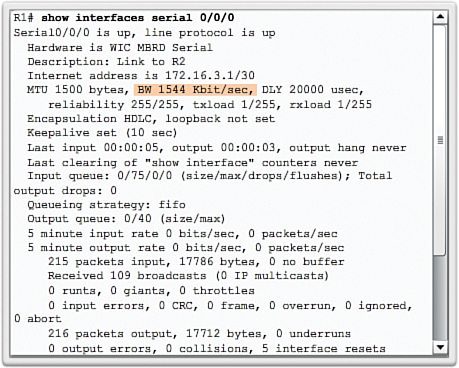
Note
The entire output in Figure 6-37 can be viewed in the online course on page 6.2.3.4 graphic number 2.
The following output displays the serial 0/0/1 interface settings for R1. It also confirms that the interface is using the default interface bandwidth of 1,544 kb/s.
R1# show interfaces serial 0/0/1 | include BW
MTU 1500 bytes, BW 1544 Kbit/sec, DLY 20000 usec,
R1#
According to the reference topology, this should be set to 64 kb/s. Therefore, the R1 Serial 0/0/1 interface must be adjusted.
Figure 6-38 displays the resulting cost metric of 647, which is based on the reference bandwidth set to 1,000,000,000 b/s and the default interface bandwidth of 1,544 kb/s (1,000,000,000 / 1,544,000).
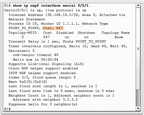
Note
The entire output in Figure 6-38 can be viewed in the online course on page 6.2.3.4 graphic number 4.
Adjusting the Interface Bandwidths (6.2.3.5)
To adjust the interface bandwidth, use the bandwidth kilobits interface configuration command. Use the no bandwidth command to restore the default value.
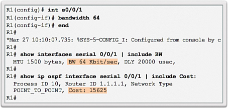
The example in Figure 6-39 adjusts the R1 Serial 0/0/1 interface bandwidth to 64 kb/s. A quick verification confirms that the interface bandwidth setting is now 64 kb/s.
The bandwidth must be adjusted at each end of the serial links, therefore:
![]() R2 requires its S0/0/1 interface to be adjusted to 1,024 kb/s.
R2 requires its S0/0/1 interface to be adjusted to 1,024 kb/s.
![]() R3 requires its Serial 0/0/0 interface to be adjusted to 64 kb/s and its Serial 0/0/1 interface to be adjusted to 1,024 kb/s.
R3 requires its Serial 0/0/0 interface to be adjusted to 64 kb/s and its Serial 0/0/1 interface to be adjusted to 1,024 kb/s.
![]() Activity 6.2.3.5: Adjusting Interface Bandwidths
Activity 6.2.3.5: Adjusting Interface Bandwidths
Go to the online course to use the Syntax Checker in the second graphic to adjust the serial interface of R2 and R3.
Note
A common misconception for students who are new to networking and the Cisco IOS is to assume that the bandwidth command changes the physical bandwidth of the link. The command only modifies the bandwidth metric used by EIGRP and OSPF. The command does not modify the actual bandwidth on the link.
Manually Setting the OSPF Cost (6.2.3.6)
As an alternative to setting the default interface bandwidth, the cost can be manually configured on an interface using the ip ospf cost value interface configuration command.
An advantage of configuring a cost over setting the interface bandwidth is that the router does not have to calculate the metric when the cost is manually configured. In contrast, when the interface bandwidth is configured, the router must calculate the OSPF cost based on the bandwidth. The ip ospf cost command is useful in multivendor environments where non-Cisco routers may use a metric other than bandwidth to calculate the OSPF costs.
Both the bandwidth interface command and the ip ospf cost interface command achieve the same result, which is to provide an accurate value for use by OSPF in determining the best route.
For instance, in the example in Figure 6-40, the interface bandwidth of Serial 0/0/1 is reset to the default value and the OSPF cost is manually set to 15,625. Although the interface bandwidth is reset to the default value, the OSPF cost is set as if the bandwidth was still calculated.

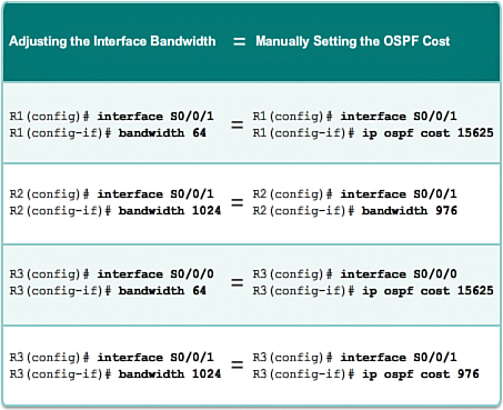
Figure 6-41 shows the two alternatives that can be used in modifying the costs of the serial links in the topology. The right side of the figure shows the ip ospf cost command equivalents of the bandwidth commands on the left.
Verify OSPF (6.2.4)
This section discusses the commands used for basic verification and troubleshooting of OSPFv2.
Verify OSPF Neighbors (6.2.4.1)
Use the show ip ospf neighbor command to verify that the router has formed an adjacency with its neighboring routers. If the router ID of the neighboring router is not displayed, or if it does not show as being in a state of FULL, the two routers have not formed an OSPF adjacency.
If two routers do not establish adjacency, link-state information is not exchanged. Incomplete LSDBs can cause inaccurate SPF trees and routing tables. Routes to destination networks may not exist, or may not be the optimum path.
Figure 6-42 displays the neighbor adjacency of R1.

For each neighbor, this command displays the following output:
![]() Neighbor ID: The router ID of the neighboring router.
Neighbor ID: The router ID of the neighboring router.
![]() Pri: The OSPF priority of the interface. This value is used in the DR and BDR election.
Pri: The OSPF priority of the interface. This value is used in the DR and BDR election.
![]() State: The OSPF state of the interface. FULL state means that the router and its neighbor have identical OSPF LSDBs. On multi-access networks, such as Ethernet, two routers that are adjacent may have their states displayed as 2WAY. The dash indicates that no DR or BDR is required because of the network type.
State: The OSPF state of the interface. FULL state means that the router and its neighbor have identical OSPF LSDBs. On multi-access networks, such as Ethernet, two routers that are adjacent may have their states displayed as 2WAY. The dash indicates that no DR or BDR is required because of the network type.
![]() Dead Time: The amount of time remaining that the router waits to receive an OSPF Hello packet from the neighbor before declaring the neighbor down. This value is reset when the interface receives a Hello packet.
Dead Time: The amount of time remaining that the router waits to receive an OSPF Hello packet from the neighbor before declaring the neighbor down. This value is reset when the interface receives a Hello packet.
![]() Address: The IPv4 address of the neighbor’s interface to which this router is directly connected.
Address: The IPv4 address of the neighbor’s interface to which this router is directly connected.
![]() Interface: The interface on which this router has formed adjacency with the neighbor.
Interface: The interface on which this router has formed adjacency with the neighbor.
![]() Activity 6.2.4.1: Verifying OSPF Neighbors
Activity 6.2.4.1: Verifying OSPF Neighbors
Go to the online course to use the Syntax Checker in the third graphic to verify the R2 and R3 neighbors using the show ip ospf neighbor command.
Two routers may not form an OSPF adjacency if:
![]() The subnet masks do not match, causing the routers to be on separate networks.
The subnet masks do not match, causing the routers to be on separate networks.
![]() OSPF Hello or Dead Timers do not match.
OSPF Hello or Dead Timers do not match.
![]() OSPF network types do not match.
OSPF network types do not match.
![]() There is a missing or incorrect OSPF network command.
There is a missing or incorrect OSPF network command.
Verify OSPF Protocol Settings (6.2.4.2)
As shown in Figure 6-43, the show ip protocols command is a quick way to verify vital OSPF configuration information. This includes the OSPF process ID, the router ID, networks the router is advertising, the neighbors the router is receiving updates from, and the default administrative distance, which is 110 for OSPF.
![]() Activity 6.2.4.2: Verifying OSPF Protocol Settings
Activity 6.2.4.2: Verifying OSPF Protocol Settings
Go to the online course to use the Syntax Checker in the second graphic to verify the OSPF protocol settings of R2 and R3 using the show ip protocols command.
Verify OSPF Process Information (6.2.4.3)
![]()
Areas
The show ip ospf command can also be used to examine the OSPF process ID and router ID, as shown in Figure 6-44. This command displays the OSPF area information and the last time the SPF algorithm was calculated.
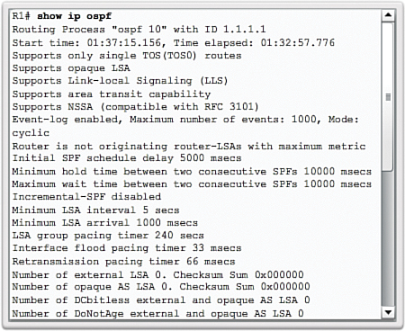
Note
The entire output in Figure 6-44 can be viewed in the online course on page 6.2.4.3 graphic number 2.
![]() Activity 6.2.4.3: Verifying OSPF Process Information
Activity 6.2.4.3: Verifying OSPF Process Information
Go to the online course to use the Syntax Checker in the second graphic to verify the OSPF process of R2 and R3 using the show ip ospf command.
Verify OSPF Interface Settings (6.2.4.4)
The quickest way to verify OSPF interface settings is to use the show ip ospf interface command. This command provides a detailed list for every OSPF-enabled interface. The command is useful to determine whether the network statements were correctly composed.
To get a summary of OSPF-enabled interfaces, use the show ip ospf interface brief command, as shown in Figure 6-45.

![]() Activity 6.2.4.4: Verifying OSPF Interface Settings
Activity 6.2.4.4: Verifying OSPF Interface Settings
Go to the online course to use the Syntax Checker in the second graphic to retrieve and view a summary of OSPF-enabled interfaces on R2 and R3 using the show ip ospf interface brief command and the show ip ospf interface serial 0/0/1 command.
![]() Lab 6.2.4.5: Configuring Basic Single-Area OSPFv2
Lab 6.2.4.5: Configuring Basic Single-Area OSPFv2
In this lab, you will complete the following objectives:
![]() Part 1: Build the Network and Configure Basic Device Settings
Part 1: Build the Network and Configure Basic Device Settings
![]() Part 2: Configure and Verify OSPF Routing
Part 2: Configure and Verify OSPF Routing
![]() Part 3: Change Router ID Assignments
Part 3: Change Router ID Assignments
![]() Part 4: Configure OSPF Passive Interfaces
Part 4: Configure OSPF Passive Interfaces
![]() Part 5: Change OSPF Metrics
Part 5: Change OSPF Metrics
Configure Single-Area OSPFv3 (6.3)
OSPFv3 is operationally similar to OSPFv2. They both have the same data structures and operational features. However, OSPFv3 is configured differently than OSPFv2. This topic discusses similarities and differences between OSPFv2 and OSPFv3.
OSPFv3 (6.3.1.1)
OSPFv3 is the OSPFv2 equivalent for exchanging IPv6 prefixes. Recall that in IPv6, the network address is referred to as the prefix and the subnet mask is called the prefix-length.
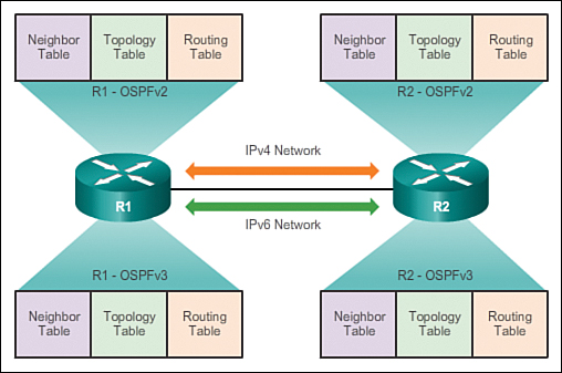
Similar to its IPv4 counterpart, OSPFv3 exchanges routing information to populate the IPv6 routing table with remote prefixes, as shown in Figure 6-46.
Note
With the OSPFv3 Address Families feature, OSPFv3 includes support for both IPv4 and IPv6.
OSPFv2 runs over the IPv4 network layer, communicating with other OSPF IPv4 peers, and advertising only IPv4 routes.
OSPFv3 has the same functionality as OSPFv2, but uses IPv6 as the network layer transport, communicating with OSPFv3 peers and advertising IPv6 routes. OSPFv3 also uses the SPF algorithm as the computation engine to determine the best paths throughout the routing domain.
As with all IPv6 routing protocols, OSPFv3 has separate processes from its IPv4 counterpart. The processes and operations are basically the same as in the IPv4 routing protocol, but run independently. OSPFv2 and OSPFv3 each have separate adjacency tables, OSPF topology tables, and IP routing tables, as shown in Figure 6-46.
The OSPFv3 configuration and verification commands are similar to those used in OSPFv2.
Similarities Between OSPFv2 and OSPFv3 (6.3.1.2)
The following are similarities between OSPFv2 and OSPFv3:
![]() Link-state: OSPFv2 and OSPFv3 are both classless link-state routing protocols.
Link-state: OSPFv2 and OSPFv3 are both classless link-state routing protocols.
![]() Routing algorithm: OSPFv2 and OSPFv3 use the SPF algorithm to make routing decisions.
Routing algorithm: OSPFv2 and OSPFv3 use the SPF algorithm to make routing decisions.
![]() Metric: The RFCs for both OSPFv2 and OSPFv3 define the metric as the cost of sending packets out the interface. OSPFv2 and OSPFv3 can be modified using the auto-cost reference-bandwidth ref-bw router configuration mode command. The command only influences the OSPF metric where it was configured. For example, if this command was entered for OSPFv3, it does not affect the OSPFv2 routing metrics.
Metric: The RFCs for both OSPFv2 and OSPFv3 define the metric as the cost of sending packets out the interface. OSPFv2 and OSPFv3 can be modified using the auto-cost reference-bandwidth ref-bw router configuration mode command. The command only influences the OSPF metric where it was configured. For example, if this command was entered for OSPFv3, it does not affect the OSPFv2 routing metrics.
![]() Areas: The concept of multiple areas in OSPFv3 is the same as in OSPFv2. Multiareas minimize link-state flooding and provide better stability with the OSPF domain.
Areas: The concept of multiple areas in OSPFv3 is the same as in OSPFv2. Multiareas minimize link-state flooding and provide better stability with the OSPF domain.
![]() OSPF packet types: OSPFv3 uses the same five basic packet types as OSPFv2 (Hello, DBD, LSR, LSU, and LSAck).
OSPF packet types: OSPFv3 uses the same five basic packet types as OSPFv2 (Hello, DBD, LSR, LSU, and LSAck).
![]() Neighbor discovery mechanism: The neighbor state machine, including the list of OSPF neighbor states and events, remains unchanged. OSPFv2 and OSPFv3 use the Hello mechanism to learn about neighboring routers and form adjacencies. However, in OSPFv3, there is no requirement for matching subnets to form neighbor adjacencies. This is because neighbor adjacencies are formed using link-local addresses, not global unicast addresses.
Neighbor discovery mechanism: The neighbor state machine, including the list of OSPF neighbor states and events, remains unchanged. OSPFv2 and OSPFv3 use the Hello mechanism to learn about neighboring routers and form adjacencies. However, in OSPFv3, there is no requirement for matching subnets to form neighbor adjacencies. This is because neighbor adjacencies are formed using link-local addresses, not global unicast addresses.
![]() DR/BDR election process: The DR/BDR election process remains unchanged in OSPFv3.
DR/BDR election process: The DR/BDR election process remains unchanged in OSPFv3.
![]() Router ID: Both OSPFv2 and OSPFv3 use a 32-bit number for the router ID represented in dotted-decimal notation. Typically this is an IPv4 address. The OSPF router-id command must be used to configure the router ID. The process in determining the 32-bit router ID is the same in both protocols. Use an explicitly configured router ID; otherwise, the highest loopback IPv4 address becomes the router ID.
Router ID: Both OSPFv2 and OSPFv3 use a 32-bit number for the router ID represented in dotted-decimal notation. Typically this is an IPv4 address. The OSPF router-id command must be used to configure the router ID. The process in determining the 32-bit router ID is the same in both protocols. Use an explicitly configured router ID; otherwise, the highest loopback IPv4 address becomes the router ID.
![]() Advertises: OSPFv2 advertises IPv4 routes, whereas OSPFv3 advertises routes for IPv6.
Advertises: OSPFv2 advertises IPv4 routes, whereas OSPFv3 advertises routes for IPv6.
![]() Source address: OSPFv2 messages are sourced from the IPv4 address of the exit interface. In OSPFv3, OSPF messages are sourced using the link-local address of the exit interface.
Source address: OSPFv2 messages are sourced from the IPv4 address of the exit interface. In OSPFv3, OSPF messages are sourced using the link-local address of the exit interface.
![]() All OSPF Routers multicast address: OSPFv2 uses 224.0.0.5, whereas OSPFv3 uses FF02::5.
All OSPF Routers multicast address: OSPFv2 uses 224.0.0.5, whereas OSPFv3 uses FF02::5.
![]() DR/BDR multicast address: OSPFv2 uses 224.0.0.6, whereas OSPFv3 uses FF02::6.
DR/BDR multicast address: OSPFv2 uses 224.0.0.6, whereas OSPFv3 uses FF02::6.
![]() Advertise networks: OSPFv2 advertises networks using the network router configuration command, whereas OSPFv3 uses the ipv6 ospf process-id area area-id interface configuration command.
Advertise networks: OSPFv2 advertises networks using the network router configuration command, whereas OSPFv3 uses the ipv6 ospf process-id area area-id interface configuration command.
![]() IP unicast routing: Enabled, by default, in IPv4, whereas the ipv6 unicastrouting global configuration command must be configured.
IP unicast routing: Enabled, by default, in IPv4, whereas the ipv6 unicastrouting global configuration command must be configured.
![]() Authentication: OSPFv2 uses either plaintext authentication or MD5 authentication. OSPFv3 uses IPv6 authentication.
Authentication: OSPFv2 uses either plaintext authentication or MD5 authentication. OSPFv3 uses IPv6 authentication.
Table 6-7 highlights the differences between OSPFv2 and OSPFv3

Link-Local Addresses (6.3.1.4)
Routers running a dynamic routing protocol, such as OSPF, exchange messages between neighbors on the same subnet or link. Routers only need to send and receive routing protocol messages with their directly connected neighbors. These messages are always sent from the source IPv4 address of the router doing the forwarding.
IPv6 link-local addresses are ideal for this purpose. An IPv6 link-local address enables a device to communicate with other IPv6-enabled devices on the same link, and only on that link (subnet). Packets with a source or destination link-local address cannot be routed beyond the link from where the packet originated.
As shown in Figure 6-47, OSPFv3 messages are sent using:
![]() Source IPv6 address: This is the IPv6 link-local address of the exit interface.
Source IPv6 address: This is the IPv6 link-local address of the exit interface.
![]() Destination IPv6 address: OSPFv3 packets can be sent to a unicast address using the neighbor IPv6 link-local address. They can also be sent using a multicast address. The FF02::5 address is the All OSPF Routers address, while FF02::6 is the DR/BDR multicast address.
Destination IPv6 address: OSPFv3 packets can be sent to a unicast address using the neighbor IPv6 link-local address. They can also be sent using a multicast address. The FF02::5 address is the All OSPF Routers address, while FF02::6 is the DR/BDR multicast address.

![]() Activity 6.3.1.5: Compare and Contrast OSPFv2 and OSPFv3
Activity 6.3.1.5: Compare and Contrast OSPFv2 and OSPFv3
Go to the online course to perform this practice activity.
Configuring OSPFv3 (6.3.2)
![]()
OSPFv3 Configuration and Verification
![]()
Lesson 3: OSPFv3 Configuration
This section discusses the commands used for configuring basic single-area OSPFv3.
OSPFv3 Network Topology (6.3.2.1)
![]()
OSPFv3 Configuration with IPv6 Example
Figure 6-48 displays the network topology that is used to configure OSPFv3.

The following shows the configuration of IPv6 unicast routing and the configuration of the global unicast address for the Gigabit Ethernet 0/0 and Serial 0/0/0 interfaces of R1, as identified in Figure 6-48. Assume that the interfaces of R2 and R3 have also been configured with their global unicast addresses, as identified in the referenced topology.
R1(config)# ipv6 unicast-routing
R1(config)#
R1(config)# interface GigabitEthernet 0/0
R1(config-if)# description R1 LAN
R1(config-if)# ipv6 address 2001:DB8:CAFE:1::1/64
R1(config-if)# no shut
R1(config-if)#
R1(config-if)# interface Serial0/0/0
R1(config-if)# description Link to R2
R1(config-if)# ipv6 address 2001:DB8:CAFE:A001::1/64
R1(config-if)# clock rate 128000
R1(config-if)# no shut
R1(config-if)#
R1(config-if)# interface Serial0/0/1
R1(config-if)# description Link to R3
R1(config-if)# ipv6 address 2001:DB8:CAFE:A003::1/64
R1(config-if)# no shut
R1(config-if)# end
R1#
In this topology, none of the routers have IPv4 addresses configured. A network with router interfaces configured with IPv4 and IPv6 addresses is referred to as dual-stacked. A dual-stacked network can have OSPFv2 and OSPFv3 simultaneously enabled.
The steps to configure basic OSPFv3 in a single area are:
Step 1. Enable IPv6 unicast routing: ipv6 unicast-routing
Step 2. (Optional) Configure link-local addresses.
Step 3. Configure a 32-bit router ID in OSPFv3 router configuration mode using the router-id rid command.
Step 4. Configure optional routing specifics such as adjusting the reference bandwidth.
Step 5. Configure optional OSPFv3 interface-specific settings.
Step 6. Adjust the interface bandwidth.
Step 7. Enable IPv6 on the interface using the ipv6 ospf area interface configuration command.
Link-Local Addresses (6.3.2.2)
In Figure 6-49, the output of the show ipv6 interface brief command confirms that the correct global IPv6 addresses have been successfully configured and that the interfaces are enabled. Also, notice that each interface automatically generated a link-local address, as highlighted in the figure.
Link-local addresses are automatically created when an IPv6 global unicast address is assigned to the interface. Global unicast addresses are not required on an interface; however, IPv6 link-local addresses are.

Unless configured manually, Cisco routers create the link-local address using the FE80::/10 prefix and the EUI-64 process. EUI-64 involves using the 48-bit Ethernet MAC address, inserting FFFE in the middle, and flipping the seventh bit. For serial interfaces, Cisco uses the MAC address of an Ethernet interface. Notice in Figure 6-49 that all three interfaces are using the same link-local address.
Assigning Link-Local Addresses (6.3.2.3)
Link-local addresses created using the EUI-64 format or, in some cases, random interface IDs, make it difficult to recognize and remember those addresses. Because IPv6 routing protocols use IPv6 link-local addresses for unicast addressing and next-hop address information in the routing table, it is common practice to make the link-local address an easily recognizable address.
Configuring the link-local address manually provides the ability to create an address that is recognizable and easier to remember. As well, a router with several interfaces can assign the same link-local address to each IPv6 interface. This is because the link-local address is only required for local communications.
Link-local addresses can be configured manually by using the same interface command used to create IPv6 global unicast addresses, but appending the link-local keyword to the ipv6 address command.
A link-local address has a prefix within the range FE80 to FEBF. When an address begins with this hextet (16-bit segment), the link-local keyword must follow the address.
The following example configures the same link-local address FE80::1 on the three R1 interfaces. FE80::1 was chosen to make it easy to remember the link-local addresses of R1.
R1(config)# interface GigabitEthernet 0/0
R1(config-if)# ipv6 address fe80::1 link-local
R1(config-if)# exit
R1(config)# interface Serial0/0/0
R1(config-if)# ipv6 address fe80::1 link-local
R1(config-if)# exit
R1(config)# interface Serial0/0/1
R1(config-if)# ipv6 address fe80::1 link-local
R1(config-if)#
A quick look at the interfaces as shown in Figure 6-50 confirms that the R1 interface link-local addresses have been changed to FE80::1.
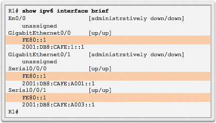
![]() Activity 6.3.2.3: Configuring Link-Local Addresses
Activity 6.3.2.3: Configuring Link-Local Addresses
Go to the online course to use the Syntax Checker in the third graphic to configure and verify link-local address FE80::2 on R2 and link-local address FE80::3 on R3.
Configuring the OSPFv3 Router ID (6.3.2.4)
Use the ipv6 router ospf process-id global configuration mode command to enter router configuration mode. The IPv6 router configuration mode prompt is different than the IPv4 router configuration mode prompt. Use the IPv6 router confirmation mode to configure global OSPFv3 parameters, such as assigning a 32-bit OSPF router ID and reference bandwidth.
IPv6 routing protocols are enabled on an interface, and not from router configuration mode, like their IPv4 counterparts. The network IPv4 router configuration mode command does not exist in IPv6.
Like OSPFv2, the process-id value is a number between 1 and 65,535 and is chosen by the network administrator. The process-id value is locally significant, which means that it does not have to match other OSPF routers to establish adjacencies with those neighbors.
OSPFv3 requires a 32-bit router ID to be assigned before OSPF can be enabled on an interface. The logic diagram in Figure 6-51 displays how a router ID is chosen. Like OSPFv2, OSPFv3 uses:
![]() An explicitly configured router ID first.
An explicitly configured router ID first.
![]() If none are configured, then the router uses the highest configured IPv4 address of a loopback interface.
If none are configured, then the router uses the highest configured IPv4 address of a loopback interface.
![]() If none are configured, then the router uses the highest configured IPv4 address of an active interface.
If none are configured, then the router uses the highest configured IPv4 address of an active interface.
![]() If there are no sources of IPv4 addresses on a router, then the router displays a console message to configure the router ID manually.
If there are no sources of IPv4 addresses on a router, then the router displays a console message to configure the router ID manually.
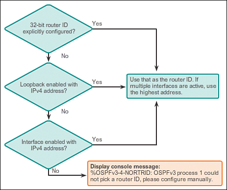
Note
For consistency, all three routers use the process ID of 10.
As shown in the topology in Figure 6-52, routers R1, R2, and R3 are to be assigned the router IDs indicated. The router-id rid command used to assign a router ID in OSPFv2 is the same command used in OSPFv3.

The example in Figure 6-53:
![]() Enters the router OSPFv3 configuration mode. Notice how the router prompt is different than the default IPv4 routing protocol mode router prompt. Also notice how an informational console message appeared when the OSPFv3 router configuration mode was accessed.
Enters the router OSPFv3 configuration mode. Notice how the router prompt is different than the default IPv4 routing protocol mode router prompt. Also notice how an informational console message appeared when the OSPFv3 router configuration mode was accessed.
![]() Assigns the router ID 1.1.1.1.
Assigns the router ID 1.1.1.1.
![]() Adjusts the reference bandwidth to 1,000,000,000 b/s (1 Gb/s), because there are Gigabit Ethernet links in the network. Notice the information console message that this command must be configured on all routers in the routing domain.
Adjusts the reference bandwidth to 1,000,000,000 b/s (1 Gb/s), because there are Gigabit Ethernet links in the network. Notice the information console message that this command must be configured on all routers in the routing domain.
![]() The show ipv6 protocols command is used to verify that the OSPFv3 process ID 10 is using the router ID 1.1.1.1.
The show ipv6 protocols command is used to verify that the OSPFv3 process ID 10 is using the router ID 1.1.1.1.
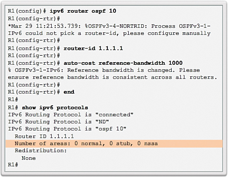
![]() Activity 6.3.2.4: Assigning a Router ID
Activity 6.3.2.4: Assigning a Router ID
Go to the online course to use the Syntax Checker in the fourth graphic to configure global OSPFv3 settings on R2 and R3.
Modifying an OSPFv3 Router ID (6.3.2.5)
Router IDs sometimes must be changed, for example, if the network administrator has established a new router ID identification scheme. However, after an OSPFv3 router establishes a router ID, that router ID cannot be changed until the router is reloaded or the OSPF process is cleared.
In the following output, notice that the current router ID is 10.1.1.1. The OSPFv3 router ID should be 1.1.1.1.
R1# show ipv6 protocols
IPv6 Routing Protocol is "connected"
IPv6 Routing Protocol is "ND"
IPv6 Routing Protocol is "ospf 10"
Router ID 10.1.1.1
Number of areas: 0 normal, 0 stub, 0 nssa
Redistribution:
None
R1#
The following assigns the router ID 1.1.1.1 to R1:
R1(config)# ipv6 router ospf 10
R1(config-rtr)# router-id 1.1.1.1
R1(config-rtr)# end
R1#
Note
Clearing the OSPF process is the preferred method to reset the router ID.
The following clears the OSPF routing process using the clear ipv6 ospf process privileged EXEC mode command. Doing this forces OSPF on R1 to renegotiate neighbor adjacencies using the new router ID.
R1# clear ipv6 ospf process
Reset selected OSPFv3 processes? [no]: y
R1#
R1# show ipv6 protocols
IPv6 Routing Protocol is "connected"
IPv6 Routing Protocol is "ND"
IPv6 Routing Protocol is "ospf 10"
Router ID 1.1.1.1
Number of areas: 0 normal, 0 stub, 0 nssa
Redistribution:
None
R1#
The show ipv6 protocols command verifies that the router ID has changed.
![]() Activity 6.3.2.5: Modifying the Router ID
Activity 6.3.2.5: Modifying the Router ID
Go to the online course to use the Syntax Checker in the fourth graphic to modify the router ID for R1.
Enabling OSPFv3 on Interfaces (6.3.2.6)
OSPFv3 uses a different method to enable an interface for OSPF. Instead of using the network router configuration mode command to specify matching interface addresses, OSPFv3 is configured directly on the interface.
To enable OSPFv3 on an interface, use the ipv6 ospf process-id area area-id interface configuration mode command.
The process-id value identifies the specific routing process and must be the same as the process ID used to create the routing process in the ipv6 router ospf process-id command.
The area-id value is the area to be associated with the OSPFv3 interface. Although any value could have been configured for the area, 0 was selected because area 0 is the backbone area to which all other areas must attach, as shown in Figure 6-54. This helps in the migration to multiarea OSPF, if the need arises.
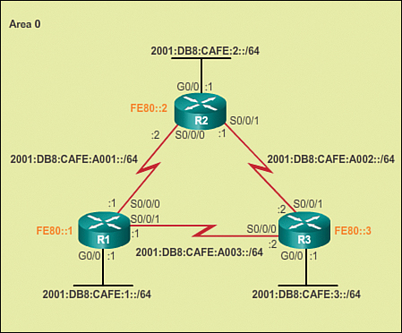
In Figure 6-55, OSPFv3 is enabled on the R1 interfaces using the ipv6 ospf 10 area 0 command. The show ipv6 ospf interface brief command displays the active OSPFv3 interfaces.
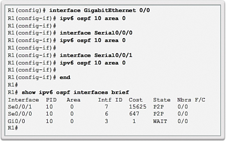
![]() Activity 6.3.2.6: Enable OSPFv3 on the R2 and R3 Interfaces
Activity 6.3.2.6: Enable OSPFv3 on the R2 and R3 Interfaces
Go to the online course to use the Syntax Checker in the third graphic to enable OSPFv3 on the R2 and R3 interfaces.
Verify OSPFv3 (6.3.3)
![]()
Verifying OSPFv3 Operation
This section discusses the commands used for basic verification and troubleshooting of OSPFv3.
Verify OSPFv3 Neighbors (6.3.3.1)
Use the show ipv6 ospf neighbor command to verify that the router has formed an adjacency with its neighboring routers. If the router ID of the neighboring router is not displayed, or if it does not show as being in a state of FULL, the two routers have not formed an OSPF adjacency.
If two routers do not establish a neighbor adjacency, link-state information is not exchanged. Incomplete LSDBs can cause inaccurate SPF trees and routing tables. Routes to destination networks may not exist or may not be the optimum path.
Figure 6-56 displays the neighbor adjacency of R1. For each neighbor, this command displays the following output:
![]() Neighbor ID: The router ID of the neighboring router.
Neighbor ID: The router ID of the neighboring router.
![]() Pri: The OSPF priority of the interface. Value is used in the DR and BDR election.
Pri: The OSPF priority of the interface. Value is used in the DR and BDR election.
![]() State: The OSPF state of the interface. FULL state means that the router and its neighbor have identical OSPF LSDBs. On multi-access networks such as Ethernet, two routers that are adjacent may have their states displayed as 2WAY. The dash indicates that no DR or BDR is required because of the network type.
State: The OSPF state of the interface. FULL state means that the router and its neighbor have identical OSPF LSDBs. On multi-access networks such as Ethernet, two routers that are adjacent may have their states displayed as 2WAY. The dash indicates that no DR or BDR is required because of the network type.
![]() Dead Time: The amount of time remaining that the router waits to receive an OSPF Hello packet from the neighbor before declaring the neighbor down. This value is reset when the interface receives a Hello packet.
Dead Time: The amount of time remaining that the router waits to receive an OSPF Hello packet from the neighbor before declaring the neighbor down. This value is reset when the interface receives a Hello packet.
![]() Interface ID: The interface ID or link ID.
Interface ID: The interface ID or link ID.
![]() Interface: The interface on which this router has formed adjacency with the neighbor.
Interface: The interface on which this router has formed adjacency with the neighbor.
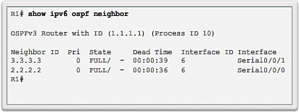
![]() Activity 6.3.3.1: Verifying OSPFv3 Neighbors for R2 and R3
Activity 6.3.3.1: Verifying OSPFv3 Neighbors for R2 and R3
Go to the online course to use the Syntax Checker in the second graphic to verify the R2 and R3 neighbors using the show ipv6 ospf neighbor command.
Verify OSPFv3 Protocol Settings (6.3.3.2)
As shown in the following output, the show ipv6 protocols command is a quick way to verify vital OSPFv3 configuration information, including the OSPF process ID, the router ID, and the interfaces enabled for OSPFv3:
R1# show ipv6 protocols
IPv6 Routing Protocol is "connected"
IPv6 Routing Protocol is "ND"
IPv6 Routing Protocol is "ospf 10"
Router ID 1.1.1.1
Number of areas: 1 normal, 0 stub, 0 nssa
Interfaces (Area 0):
Serial0/0/1
Serial0/0/0
GigabitEthernet0/0
Redistribution:
None
R1#
![]() Activity 6.3.3.2: Verifying OSPFv3 Protocol Settings on R2 and R3
Activity 6.3.3.2: Verifying OSPFv3 Protocol Settings on R2 and R3
Go to the online course to use the Syntax Checker in the second graphic to verify the OSPF protocol settings of R2 and R3 using the show ipv6 protocols command.
Use the show ipv6 ospf command to also examine the OSPFv3 process ID and router ID. This command displays the OSPF area information and the last time the SPF algorithm was calculated.
Verify OSPFv3 Interfaces (6.3.3.3)
The quickest way to verify OSPF interface settings is to use the show ipv6 ospf interface command. This command provides a detailed list for every OSPF-enabled interface.
To retrieve and view a summary of OSPFv3-enabled interfaces on R1, use the show ipv6 ospf interface brief command, as shown in Figure 6-57.

![]() Activity 6.3.3.3: Verifying OSPFv3 Interfaces on R2 and R3
Activity 6.3.3.3: Verifying OSPFv3 Interfaces on R2 and R3
Go to the online course to use the Syntax Checker in the second graphic to view a summary of OSPF-enabled interfaces on R2 and R3 using the show ipv6 ospf interface brief command. Notice that specifying the interface name as done in the show ipv6 ospf interface serial command provides detailed OSPF information.
Verify the IPv6 Routing Table (6.3.3.4)
In Figure 6-58, the show ipv6 route ospf command provides specifics about OSPF routes in the routing table.

![]() Activity 6.3.3.4: Verifying the IPv6 Routing Table of R2 and R3
Activity 6.3.3.4: Verifying the IPv6 Routing Table of R2 and R3
Go to the online course to use the Syntax Checker in the second graphic to verify the OSPFv3 routing table of R2 and R3, by using the show ipv6 route ospf command.
![]() Packet Tracer Activity 6.3.3.5: Configuring Basic OSPFv3
Packet Tracer Activity 6.3.3.5: Configuring Basic OSPFv3
In this activity, the IPv6 addressing is already configured. You are responsible for configuring the three-router topology with a basic single-area OSPFv3, and then verifying connectivity between end devices.
![]() Lab 6.3.3.6: Configuring Basic Single-Area OSPFv3
Lab 6.3.3.6: Configuring Basic Single-Area OSPFv3
In this lab, you will complete the following objectives:
![]() Part 1: Build the Network and Configure Basic Device Settings
Part 1: Build the Network and Configure Basic Device Settings
![]() Part 2: Configure OSPFv3 Routing
Part 2: Configure OSPFv3 Routing
![]() Part 3: Configure OSPFv3 Passive Interfaces
Part 3: Configure OSPFv3 Passive Interfaces
Summary (6.4)
![]() Class Activity 6.4.1.1: Stepping Through OSPFv3
Class Activity 6.4.1.1: Stepping Through OSPFv3
This class activity is designed for groups of three students. The objective is to review the Shortest Path First (SPF) routing process.
You will design and address a network, communicate the network address scheme and operation of network links to your group members, and compute the SPF.
Complete the steps as shown on the PDF for this class activity.
If you have time, share your network design and Open Shortest Path First (OSPF) process with another group.
![]() Packet Tracer Activity 6.4.1.2: Skills Integration Challenge
Packet Tracer Activity 6.4.1.2: Skills Integration Challenge
In this Skills Integration Challenge, your focus is OSPFv2 and OSPFv3 configurations. You will configure IP addressing for all devices. Then you will configure OSPFv2 routing for the IPv4 portion of the network and OSPFv3 routing for the IPv6 portion of the network. One router will be configured with both IPv4 and IPv6 configurations. Finally, you will verify your configurations and test connectivity between end devices.
The current version of OSPF for IPv4 is OSPFv2, introduced in RFC 1247 and updated in RFC 2328 by John Moy. In 1999, OSPFv3 for IPv6 was published in RFC 2740.
OSPF is a classless, link-state routing protocol with a default administrative distance of 110, and is denoted in the routing table with a route source code of O.
OSPF is enabled with the router ospf process-id global configuration mode command. The process-id value is locally significant, which means that it does not need to match other OSPF routers to establish adjacencies with those neighbors.
The network command used with OSPF has the same function as when used with other IGP routing protocols, but with slightly different syntax. The wildcard-mask value is the inverse of the subnet mask, and the area-id value should be set to 0 for single-area OSPF.
By default, OSPF Hello packets are sent every 10 seconds on multi-access and point-to-point segments and every 30 seconds on NBMA segments (Frame Relay, X.25, ATM), and are used by OSPF to establish neighbor adjacencies. The Dead interval is four times the Hello interval, by default.
For routers to become adjacent, their Hello Interval, Dead interval, network types, and subnet masks must match. Use the show ip ospf neighbors command to verify OSPF adjacencies.
OSPF elects a DR to act as the collection and distribution point for LSAs sent and received in the multi-access network. A BDR is elected to assume the role of the DR should the DR fail. All other routers are known as DROTHERs. All routers send their LSAs to the DR, which then floods the LSA to all other routers in the multi-access network.
The show ip protocols command is used to verify important OSPF configuration information, including the OSPF process ID, the router ID, and the networks the router is advertising.
OSPFv3 is enabled on an interface and not under router configuration mode. OSPFv3 needs link-local addresses to be configured. IPv6 unicast routing must be enabled for OSPFv3. A 32-bit router ID is required before an interface can be enabled for OSPFv3.
Practice
The following activities provide practice with the topics introduced in this chapter. The Labs and Class Activities are available in the companion Routing Protocols Lab Manual (978-1-58713-322-0). The Packet Tracer Activities PKA files are found in the online course.
Class Activity 6.4.1.1: Stepping Through OSPFv3
Lab 6.3.3.6: Configuring Basic Single-Area OSPFv3
Packet Tracer Activity 6.3.3.5: Configuring Basic OSPFv3
Packet Tracer Activity 6.4.1.2: Skills Integration Challenge
Check Your Understanding Questions
Complete all the review questions listed here to test your understanding of the topics and concepts in this chapter. The appendix, “Answers to the ‘Check Your Understanding’ Questions,” lists the answers.
1. Which of the following statements are true regarding routing protocols that use the link-state routing algorithm? (Choose three.)
A. They are known collectively as link-state routing protocols.
B. They learn routes and send them to directly connected neighbors.
C. They maintain a database of the network topology.
D. They are based on the Dijkstra algorithm.
E. They are considered a good choice for small networks with low-end routers.
2. What reasons would a network administrator have for using loopback interfaces when configuring OSPF? (Choose two.)
A. Loopbacks are logical interfaces and do not go down.
B. Only loopback addresses can be used for an OSPF router ID.
C. Loopback interfaces are used to set the OSPF metric.
D. The loopback address will be used as the router ID, overriding the physical IP address values.
E. OSPF error checking is enabled by loopback addresses.
F. The loopback address will override the configured router priority value.
3. In which of the following types of networks will OSPF Designated Routers not be elected? (Choose two.)
A. Point to point
B. Point to multipoint
C. Broadcast multi-access
D. Nonbroadcast multiaccess
4. After routers have converged, which OSPF component is identical on all OSPF routers in an area?
A. Adjacency database
B. Link-state database
C. Routing table
D. SPF tree
5. A network administrator enters the router ospf 100 command. What is the function of the number 100 in this command?
A. Autonomous system number
B. Metric
C. Process ID
D. Administrative distance
6. On a router running OSPF, what is the purpose of entering the bandwidth 56 command on a serial interface?
A. Changes the cost value
B. Functions only as a description
C. Changes the throughput of the interface to 56 kb/s
D. Is necessary for the DUAL algorithm
7. What factor does the Cisco implementation of OSPF use to pick the best route?
A. Uptime
B. Reliability
C. Bandwidth
D. Load
E. Shortest number of hops
8. Which wildcard mask would be used to advertise the 192.168.1.64/27 network as part of an OSPF configuration?
A. 0.0.0.15
B. 0.0.0.16
C. 0.0.0.31
D. 0.0.0.32
E. 255.255.255.192
F. 255.255.255.224
9. During an OSPF DR/BDR election, what is used to determine the DR or BDR when participating OSPF routers have identical interface priorities?
A. The highest OSPF process ID
B. The lowest interface IP address
C. The lowest interface cost
D. The highest router ID
10. Which packet type is invalid for OSPF?
A. Hello
B. LRU
C. LSR
D. LSAck
E. DBD
11. How do OSPFv2 and OSPFv3 differ?
A. Their metric calculation is different.
B. The Hello mechanism is different.
C. OSPFv3 has different packet types.
D. OSPFv3 authenticates differently.
E. The DR/BDR election works differently.
12. Which command is used to verify specific OSPFv3 routes in the IPv6 routing table?
13. In the router ospf command, does the process ID need to match on all routers?
14. Given the following configuration, what is the OSPF router ID of RouterA?
RouterA(config)# interface serial 0/0/0
RouterA(config-if)# ip add 192.168.2.1 255.255.255.252
RouterA(config-if)# interface loopback 0
RouterA(config-if)# ip add 10.1.1.1 255.255.255.255
RouterA(config-if)# router ospf 1
RouterA(config-router)# network 192.168.2.0 0.0.0.3 area 0
15. What command enables you to verify or determine the bandwidth value of an interface used by the OSPF metric?
16. What command enables you to modify the OSPF cost of an interface without modifying the bandwidth value of that interface?
17. What is the default Hello interval on Ethernet networks and serial point-to-point networks? What is the default Hello interval on NBMA networks?
18. What values must match before two routers will form an OSPF adjacency?
19. What problems does electing a DR and BDR solve?
20. How are the DR and BDR elected?