
Resilience for extreme scale computing
R. Gioiosa Pacific Northwest National Laboratory, Richland, WA, United States
Abstract
Supercomputing systems are essential for making progress in the areas of science and industries, from quantum mechanics, to oil and gas exploration. The ever-increasing demand of computing power has driven the development of extreme large systems that consists of millions of common-off-the-shelf components. As those systems approach technology and operational cost limits, new challenges arise, especially in the area of resilience, which make supercomputing environments extremely unstable and unreliable.
This chapter reviews the intrinsic characteristics of high-performance applications and how faults occurring in hardware propagate to memory. Next, the chapter summarizes resilience techniques commonly used in current supercomputers and supercomputing applications, both at system and algorithmic level. Finally, the chapter explores some resilience challenges expected in the exascale era and possible programming models and resilience solutions.
Keywords
Resilience; High-performance computing; Checkpointing; Silent data corruption; Operating systems; Exascale; Task programming models; Performance anomalies
1 Introduction
Supercomputers are large systems that are specifically designed to solve complex scientific and industrial challenges. Such applications span a wide range of computational intensive tasks, including quantum mechanics, weather forecasting, climate research, oil and gas exploration, molecular dynamics, and physical simulations, and require an amount of computing power and resources that go beyond what is available in general-purpose computer servers or workstations. Until the late 1990s, supercomputers were based on high-end, special-purpose components that underwent extensive testing. This approach was very expensive and limited the use of supercomputers in a few research centers around the world. To reduce the acquisition and operational costs, researchers started to build supercomputers out of “common-off-the-shelf” (COTS) components, such as those used in general-purpose desktop and laptop. This technology shift greatly reduced the cost of each supercomputer and allowed many research centers and universities to acquire mid- and large-scale systems.
Current supercomputers consist of a multitude of compute nodes interconnected through a high-speed network. Each compute node features one or more multicore/multithreaded processor chips, several memory modules, one/two network adapters, and, possibly, some local storage disks. More recently, accelerators, in the form of graphical vector units or field-programmable gate arrays (FPGA), have also made their way to mainstream supercomputing.
On the other hand, however, COTS components brought a new set of problems that makes HPC applications run in a harsh environment. First, COTS components are intrinsically more vulnerable than special-purpose components and, because of cost reasons, follow different production process and verification/validation paths than military or industry mission-critical embedded systems or server mainframes. This means that the individual probability that every single component may fail is higher than in other domains. Second, COTS components are not specifically design to solve scientific applications and their single-processor performance was lower than the vector processor, thus a larger number of processors are usually required to achieve the desired performance. Combining together an extremely large number of system components greatly increase the combined probability that at least one breaks, experience a soft error, or stop functioning completely or partially. Third, HPC workloads have been shown to be extremely heterogeneous and can possibly stress different parts of the supercomputers, such as memory, processors, or network. This heterogeneous behavior, in turn, increases the thermal and mechanical stress, effectively reducing the life span of each component and the entire system. The location and the facility where the supercomputer is installed play an important role in the resilience of the system. The cooling system of the machine room must be appropriate to reduce the temperature of densely-packet compute nodes with limited space for air flow. Modern supercomputers take cooling a step forward and provide liquid cooling solution embedded in the compute node racks. Moreover, recent studies confirm that supercomputer installed at higher altitudes, such as Cielo at Los Alamos National Laboratory (LANL), are more exposed to radiation and show higher soft error rates [1]. Finally, the mere size of current supercomputers makes it impossible to employ resilience solutions commonly used in other domains, both because of cost and practical reasons. For example, traditional resilience techniques, such double- or triple-module redundancy (DMR, TMR), are prohibitive in the context or large supercomputers because of the large number of compute nodes and compute nodes’ components. Moreover, additional redundant or hardening hardware might increase the overall cost considerably. Even a 10% increase in energy consumption might results in a large increase in the electricity bill if the system consumes a large amount of power.
Without specific and efficient resilience solutions, modern HPC systems would be extremely unstable, to the point that it is utopistic to assume that a production run of a scientific application will not incur in any error or will be able to terminate correctly. This chapter will review some of the most common resilience techniques adopted in the HPC domains, both application-specific and system-oriented. The chapter will also provide initial insights and research directions for future exascale systems.
2 Resilience in Scientific Applications
Research scientists rely on supercomputers to solve computation intensive problems that cannot be solved on single workstation because of the limited computing power or memory storage. Scientific computations usually employ double-precision floating point operations to represent physics quantities and to compute velocity and position of particles in a magnetic field, numerical approximations, temperature of fluids or material under thermal solicitation, etc. The most common representation of double-precision floating point values follows the IEEE Standard for Floating-Point Arithmetic (IEEE 754) [2]. With a finite number of bits, this format is necessarily an approximate representation of real numbers. As a consequence, rounding up errors are common during floating-point computations and must be taken into account when writing scientific code. Additionally, many scientific problems do not have a closed form that can be solved by using a direct method. In these cases, iterative methods are used to approximate the solution of the problem. In contrast to direct methods, which provide an exact solution to the problem, iterative methods produce a sequence of improving approximate solution for the problem under study. Iterative methods are said to be “convergent” if the corresponding sequence converges for given initial approximations based on a measurement of the error in the result (the residual). During the execution, iterative methods form a “correction equation” and compute the residual error. The approximation process is repeated until the residual error is small enough, which implies that the computed solution is acceptable, or until a maximum number of iterations have been reached, in which case the solution might not be acceptable.
The uncertainty introduced by the floating-point representation and the iterative approximation require scientific applications to assess the quality of the solution, often in the form of a residual error. The quality of the solution is typically reported in addition to the solution itself: for example, a molecular dynamics application might produce a final state in which the molecules have evolved and a residual error to assess the feasibility of the dynamics. By tuning the residual errors, scientists can increase the quality of the computed solution, generally at the cost of higher computing time. For example, a larger number of iteration steps might be necessary to reach an approximation with a lower residual error, i.e., a better solution.
When running in faulty environments, computation errors can also occur because of bit-flips in processor registers and functional units, or memory. Using the residual error, HPC applications can generally assess whether a fault has produced an error or if it has vanished. However, the very approximate nature of both floating-point representation and iterative, indirect mathematical methods, makes most HPC applications “naturally tolerant” to a small number of bit-flips. For example, consider the case of a bit-flip in a double-precision floating-point register. In the IEEE 754 representation, one bit indicates the sign of the number, 11 bits store the exponent, and 52 bits store the mantissa. Because of the lossy representation, a bit-flip in the mantissa may introduce only a small perturbation and, thus, has much lower chances to affect the final result than a bit flip in the exponent or the sign [3]. In the case of iterative methods, a small perturbation caused by a fault may delay the convergence of the algorithm. The application could still converge to an acceptable solution with a few more iterations or terminate with a less accurate solution. This example exposes a trade-off between performance and accuracy: given enough time, iterative methods could converge to an acceptable solution even in the presence of faults that introduce small perturbations. On the other hand, because of the fault, the application may never converge, thus it is necessary to estimate or statically determine how many extra iterations should be performed before aborting the execution. This is a difficult problem with high-risk/high-reward impact. On one hand, the applications might have run for weeks and a few more hours of work could provide a solution and avoid complete re-execution. On the other hand, the application may never converge. In the absence of mathematical foundations to estimate if and when the application will converge, the practical solution is to statically set a fixed number of maximum iterations after which the application is aborted. As the number of soft errors increases, the choice of whether to invest time and resources in the hope that the application will converge will become even more important, thus methods to estimate the probability that the application will converge are required.
For large perturbations, there is a possibility that the algorithm will never converge. In this case, the application will reach the maximum number of iterations and terminate without providing an acceptable solution. Normally, however, these impossible convergence conditions can be detected by the application itself. In these cases, the application will typically abort as soon as the condition is detected and will report an error, saving the remaining execution time. This technique is used, for example, in LULESH, a shock hydrodynamics proxy application developed by the ASCR ExMatEx Exascale Co-Design Center [4]. In particular, LULESH periodically checks the consistency of the solution and aborts if either the volume of the fluid or any element have negative values.
Compared to other classes of applications, HPC applications can be classified in the following categories:
Vanished (V): Faults are masked at the processor-level and do not propagate to memory, thus the application produces correct outputs (COs) and the entire internal memory’s state is correct.
Output not affected (ONA): Faults propagate to the application’s memory state, but the final results of the computation are still within the acceptable error margins and the application terminates within the number of iterations executed in fault-free runs.
Wrong output (WO): Faults propagate through the application’s state and corrupt the final output. The application may take longer to terminate.
Prolonged execution (PEX): Some applications may be able to tolerate corrupted memory states and still produce correct results by performing extra work to refine the current solution. These applications provide some form of inherent fault tolerance in their algorithms, though at the cost of delaying the output.
Crashed (C): Finally, faults can induce application crashes. We consider “hangs,” i.e., the cases in which the application does not terminate, in this class.
This classification extends the one previously proposed in [5–8] to account for specific HPC features. Compared to the classification presented in Chapter 2, SDCs are identified as ONA, WO, and PEX, depending on their effects on the application’s state and output. Analysis based on output variation, such as fault injection analysis, cannot distinguish V from ONA, thus we introduce the class CO to indicate the sum of V and ONA when the application produces correct results within the expected execution time. Correct results with longer executions are in PEX.
A recent study [9] shows the outcomes of injecting faults into several HPC applications from the U.S. DOE Exascale Co-Design centers,1 DOE Office of Science, and the CORAL benchmark suite.2 Fig. 1 shows the statistical result outcomes of injecting single-bit fault at architectural register level. In this experiments, each application was executed 5000 times and one single-bit fault was injected in each run into a random MPI process. Faults are injected into input or output registers of arithmetic operations, both integer and floating-point using a modified version LLFI [10], an application-level fault injector based on LLVM [11], for MPI applications. The application output is considered corrupted (WO) if it differs significantly from the fault-free execution or if the application itself reports results outside of the acceptable error boundaries. A similar analysis is presented, for a different set of applications, in [10, 12, 13].

The results in the figures show that each application present different vulnerability. Single-bit faults injected in LULESH appear to result in correct execution (CO) in over 90% of the cases, i.e., the computed solution is within the user-specified error margins. Moreover, generally, no additional iteration is performed (PEX) to achieve the result. For this application, only less than 10% of the executions result in crashes and less than 5% of the experiments produce wrong results. LAMMPS sits at the other extreme of the vulnerability spectrum, with only 40% of the experiments producing correct results within the expected number of iterations. In over 40% of the cases, the results is wrong (WO) and, in about 20% of the experiments the application crashes. While MCB and AMG2013 show results similar to LAMMPS, though they appear to be more robust, miniFE shows a large percentage of experiments (over 15% of the cases) that produce correct results but take longer to converge (PEX). These are interesting cases, as they expose a particular characteristic of scientific applications that is not necessarily present in other domains: the user could trade-off the accuracy and correctness of the computed solution for performance.
Generally, the experiments that result in crashes are mainly due to bit flips in pointers that cause the applications to access a part of the address space that has not been allocated. However, in some cases, applications may abort autonomously because the injected fault either produced an “unfeasible” value or the convergence of the algorithm is compromised beyond repair. This is the case for LULESH: if the energy computed at time step i is outside of the acceptable boundary, the application aborts the execution calling MPI_Abort() routine. As potentially wrong execution are detected earlier, the number of WO cases is limited.
The results presented in Fig. 1 and in other works [10, 12, 13] show interesting characteristics of HPC applications but do not provide the user or an intelligent runtime with actionable tools to tune the fault-tolerance mechanism during the execution of a parallel application. Moreover, statistical analysis based on output variation do not necessarily assess that a fault has not propagated into the application memory state. In fact, output analysis might be based on the residual reported by the application, which may also be a part of the output.
Fig. 2 shows an analysis of fault propagation for LULESH under the same circumstances of the experiments reported in Fig. 1. Although the results in Fig. 1 show that LULESH appears to be very robust, the plot in Fig. 2 shows that many faults propagate through the application state, even when the final outcome appears correct. The fact that the result appears to be correct, thus, does not mean that faults have not propagated but only that effects of a bit-flip may be confused with the approximation due to the use of floating point operations. Nevertheless, faults propagate in LULESH with each time step.
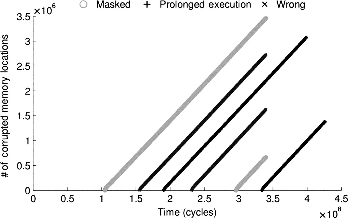
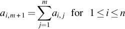
Fig. 2 provides another interesting information: faults propagate linearly in time. This information can be used to build a fault propagation model and to estimate the number of memory location corrupted by a fault detected at time tf. By using linear regression or machine learning techniques, it is possible to derive a family of linear fault propagation models (one per experiment) to estimate the number of corrupted memory locations (CML) as function of the time t:
where a expresses the propagation speed and b is the intercept with the time axis.3 The value of b for a specific experiment can be determined as:
By averaging the propagation speed factor of all experiments, it is possible to derive the fault propagation speed (FPS) factor for an application. FPS expresses how quickly a fault propagates in the application memory state and represent an intrinsic characteristic of an HPC application. FPS is an actionable metric that can be used to estimate the number of memory locations contaminated by a fault. For example, assuming that a fault is detected at time tf, then the maximum number of contaminated memory locations in an time interval [t1, t2] is:
which assumes that tf is close to the lower extreme of the interval, t1. This information can be used, for example, to decide when and if a rollback should be triggered.
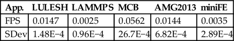
Table 1 shows the FPS values for all the application reported in Fig. 1. The table show that, when considering the speed at which faults propagates, LULESH is much more vulnerable than LAMMPS, as faults propagate at a rate of 0.0147 CML/s in the former and 0.0023 CML/s in the latter. MCB is the most vulnerable application among the ones tested. For this application faults propagate at a rate of 0.0531 CML/s.
3 System-Level Resilience
The most appealing resilience solutions, from the user prospective, are those that automatically make applications and systems tolerant to faults without or with minimal user intervention. Compared to application-specific fault tolerance solutions presented in Section 4, system-level resilience techniques provide fault-tolerance support without modifications of the application’s algorithm or structure. Applications and fault-tolerance solutions are mostly decoupled, thus the user can chose the most appropriate system-level solutions, i.e., a dynamic library, for each application or can simply use the one already provided by the supercomputer system administrator.
Among the system-level fault-tolerance techniques, checkpoint/restart solutions are the most widely used, especially in the context of recovering from hard faults, such as compute node crashes [14, 15]. Checkpointing refers to the action of recording the current total or partial state of a computation process for future use. Checkpoint/restart solutions periodically save the state of a computational application to stable/safe storage, such as a local disk or a remote filesystem storage media, so that, in the event of a failure, the application can be restarted from the most recent checkpoint. Generally, checkpoint/restart solutions work well under the following assumptions:
Fault detection: Faults can always be detected, either using hardware or software techniques, or can be safely assumed, such as in the case of a nonresponding compute node. This model is often referred to as fail-stop semantics [16].
Consistency: The state of the entire application, including all compute nodes, processes, and threads, can be stored at the same time and all in-flight communication events must be processed before the checkpoint is taken or delayed until the checkpoint is completed.
Ubiquity: In the case of a compute node failure, a checkpointed process can restart on a different node and the logical communication layer can safely be adapted to the new physical mapping.
Many properties of a checkpoint/restart solution affect the execution of parallel applications. First, the direct overhead introduced by periodically saving the state of the application takes resources that would have been used to make progress in the computation. An application that is checkpointed during the execution runs in a lock-step fashion, where all processes compute for a certain amount of time and then stop so that a consistent checkpoint can be taken. The checkpointing interval is the amount of time that intercurs between two consecutive checkpoints. Generally, the checkpointing interval is constant, especially for transparent solutions that periodically save the state of the application without user intervention. However, adaptive checkpointing intervals can be used if the application present different execution phases or if the vulnerability of the system increases. Adaptive checkpoint/restart solutions present higher complexity, thus solutions with fixed checkpointing interval are more common. The size of the checkpoint refers to the amount of data that is saved to stable storage to properly restart the application in case of failure. The size of the checkpoint strongly depends on the application’s memory footprint but is also affected by the meta-data used by the checkpoint/restart system to describe the state of the application on storage. To reduce the checkpointing size, researchers have investigated alternatives that avoid saving the entire application state (full checkpointing) but rather save only the data that has changed since the last checkpoint (incremental checkpointing). Incremental checkpointing might reduce the amount of data that needs to be saved at every checkpoint but generally increases the restarting time after a failure. In fact, it might be necessary to use more than a single checkpoint to rebuild the full state of the application, possibly starting from a full checkpoint. Moreover, whether or not incremental checkpointing is beneficial for an application depends on the memory access patterns. Several applications, such as streaming or stencil computations, tend to rewrite the entire memory space within a short amount of time, possibly shorter than the checkpointing interval. Finally, a checkpoint/restart solution is considered transparent if it does not require user intervention (except, perhaps, to set some system-level parameters, such as the checkpointing interval), or semitransparent if the user needs to provide guidance about which data structures need to be saved or when.
A general objective of any resilience solution, including checkpoint/restart systems, is to minimize the impact on the application performance and power consumption. In other terms, the amount of resources that can be dedicated to resilience, either temporally or spatially, is limited. For checkpoint/restart solutions, the two major objectives are to minimize the runtime overhead and the disk space. The former is affected by the checkpointing interval, the amount of data to be saved and the location of the storage media. Saving the checkpoint in memory or on local disk reduces the transfer time but also increases the risk of not being able to restart the application, if the entire node fails. The disk space used is mainly a function of the checkpoint size. As discussed above, incremental checkpointing can be used to minimize the size of a single checkpoint. However, more than one checkpoint needs to be stored on disk to ensure proper restart in case of failure. In the other hand, in case of full checkpoint, it could be possible to discard all the other checkpoints taken before the last.
3.1 User-Level Checkpointing
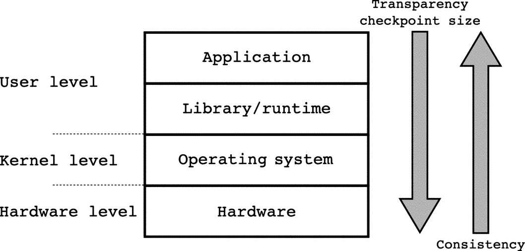
Checkpoint/restart solutions are designed and implemented at different levels of the hardware/software stack. The choice of where to implement the solution affects most of its properties, including transparency to the application, size of the state to be saved, and comprehensiveness of the state saved. Fig. 3 shows possible implementations within the hardware/software stack. At higher level, a checkpoint/restart solution can be implemented within the applications. This approach is generally expensive in terms of user effort and is seldom adopted, as many checkpoint/restart operations are common to many applications. The next step is to group together common checkpoint/restart functionalities within a user-level library. These libraries provide specific APIs to the user to instrument which data structures should be saved and when should a checkpoint be taken to guarantee consistency. Solutions implemented at this level are considered intrusive, as they require application code modifications, but are also the ones that provide the user with APIs to express which data structures are really important for the recovery of the state of the application in case of failure. The checkpoint size is generally smaller as compared to other solutions implemented at lower level. However, the user has to explicitly indicate which data structures should be saved during checkpointing and when the checkpoint should be taken to guarantee consistency. Compiler extensions can be used to ease the burden on the programmer by automatically identify loop boundaries, global/local data structure, and perform pointer analysis. The compiler can, then, either automatically instrument the application or provide a report to the user that will guide the manual instrumentation. At restart time, the user may need to provide a routine to redistribute data among the remaining processes or to fast-forward the execution of the application to the point where the most recent checkpoint was taken.
At lower level, a runtime system can be used to periodically and automatically checkpoint a parallel application. These solutions typically come in the form of a runtime library that can be preloaded before the application is started, as an extension of the programming model runtime, such as MPI [17, 18], or as compiler modules that automatically instrument the application code and link to the checkpoint/restart library for runtime support. The main advantage of this approach is the higher level of transparency and the lower level of involvement of the user, thus higher productivity. A single checkpoint/restart solution can generally be used with many applications without major effort from the programmer. It usually suffices to recompile or relink the applications against the checkpoint/restart library and set some configuration parameters, such as the checkpointing interval. The primary disadvantage is the lost of application knowledge that can be used to disambiguate which data structures are actually essential for the correct representation of the state of the application and which can be omitted from the checkpoint. The checkpoint size generally increases and, for long-running application, the space complexity may be a limiting factor.
Completely transparent runtime checkpoint/restart solutions do not require user intervention and periodically save the application state based on a timer or the occurrence of an event, such as at loop boundaries identified by the compiler. The flexibility and transparency provided by automatic checkpoint/restart runtime solutions come at the cost of a generally larger checkpoint size and increased complexity to guarantee consistency. In fact, without user intervention, it becomes difficult to distinguish the data structures that contain the application state from those that are temporal or redundant. Typically, local variables stored on the process’ stacks and read-only memory regions are omitted from the checkpoint. However, even within the heap and read-write memory regions there might be redundant or temporal data structures that need not to be saved. Consistency is also difficult to guarantee. For tightly coupled applications that often synchronize with global barriers, the checkpoint can be easily taken when the last application’s process reaches the barrier and before all processes leave it. Several automatic checkpoint/restart solutions intercepted the pMPI barrier symbol in the MPI communication library to ensure that all processes where at the same consistent state when the checkpoint was taken. Applications that often synchronize with global barriers, however, do not tend to scale well, especially on large supercomputer installations. Applications that exchange asynchronous messages and that synchronize with local barriers scale more effectively but also pose problems regarding the consistency of checkpointing. In particular, the automatic checkpointing runtime needs to ensure that there are no in-flights messages. If the checkpoint is taken when the message has left the source process but has not yet reached the destination, the message’s content would be neither in the context of the source process nor the context of the destination and it becomes lost. At restart time, there is no information about the lost message: the source process will not resend the message, as it appears already sent in its context, and the destination process will wait for a message that will never arrive, thereby possibly blocking the progress of the entire application.
3.2 Privileged-Level Checkpointing
In some cases, the application state does not contain sufficient information to seamlessly restart the system after a failure. This happens when some hardware or system software states must be restored before restarting the application. Solutions implemented at supervisor/hypervisor level, i.e., operating system (OS) or virtual machine manager (VMM) level, provide the necessary support to save the state of the entire compute node as part of the checkpoint. These solutions are capable of restoring the entire system, both hardware and application, at the point when the failure occurred. With this approach, the application does not need to be fast-forwarded to the time when the fault occurred just to set the underlying hardware and OS to the proper state.
Privileged access to hardware and software compute node information may also facilitate the gathering of the state information. The OS has unrestricted access to the state information of all processes running in a compute node and to the underlying hardware. Implementing incremental checkpoint/restart solutions based on page frame dirty bit is usually easier at this level because the OS can directly manipulate the page table entries. The OS can mark a page as dirty and as to-be-saved at the next checkpointing interval without incurring in the high overhead cost of using the mprotect() system call. A similar operation performed from a user-level library or application would involve a two-step procedure: First, the process address space needs to be protected from write access through the mprotect() system call. On attempt to modify a page, the OS will send a SIGSEV signal to the process. This signal must be intercepted by the process or checkpointing library signal handler and the page must be marked as to-be-saved. In this endeavor, the user/kernel boundary is passed twice, once from the mprotect() system call for restricting access to a page, and once from the signal handler to record that the page has been modified since the last checkpoint.
One of the OS-level checkpoint/restart solution is the Transparent Incremental Checkpointing at Kernel level, TICK [19] TICK is a fully transparent solution implemented as a Linux kernel module that provides the user with functionalities to perform both full and incremental checkpointing with extremely low overhead. As explained above, tracking dirty pages at kernel level is more efficient than at user level. TICK uses the dirty bits stored in the page table entry of each page to track which page has been modified since the last checkpoint. On the first access to a protected page, the OS triggers a page fault exception (similar to the case in which a page is protected through mprotect() system call) and TICK stores the address of the page is a bitmask so that the page can be saved at the next checkpoint.
Fig. 4 shows the runtime overhead introduced by TICK to save the full application state for two applications, SAICs Adaptive Grid Eulerian (SAGE) and Sweep3D. SAGE hydrocode is a multidimensional (1D, 2D, and 3D), multimaterial, Eulerian hydrodynamics code with adaptive mesh refinement. The code uses second order accurate numerical techniques, and is used to investigate continuous adaptive Eulerian techniques to stockpile stewardship problems. SAGE has also been applied to a variety of problems in many areas of science and engineering including water shock, energy coupling, cratering and ground shock, stemming and containment, early time front end design, explosively generated air blast, and hydrodynamic instability problems [20]. The ASCI Sweep3D benchmark is designed to replicate the behavior of particle transport codes which are executed on production machines [21]. The benchmark solves a one-group time-independent discrete ordinates neutron transport problem, calculating the flux of neutrons through each cell of a three-dimensional grid along several directions of travel. Both SAGE and Sweep3D were developed at the LANL.
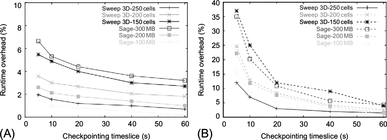
As expected, the runtime overhead decreases with the increased checkpointing interval, both for in-memory and on-disk checkpointing. However, Fig. 4A shows that, even with extremely small checkpointing intervals (5 s) the runtime overhead introduced to save the full application state in memory is less than 8%. Saving the checkpoint to disk introduces larger overhead, especially for small checkpointing intervals. For more realistic checkpointing intervals, 60 s or more, the runtime overhead is less than 4%, when saving the checkpoint in memory, and 5% when saving the checkpoint to disk. It is worth noticing that, for on-disk checkpointing, the overhead greatly reduces for checkpointing intervals larger than 10 s. This is because 10 s coincides with the normal dirty pages synchronization time interval, thus the pages containing the application checkpoint can be piggy-backed to the other dirty pages with a unique stream of data to disk.
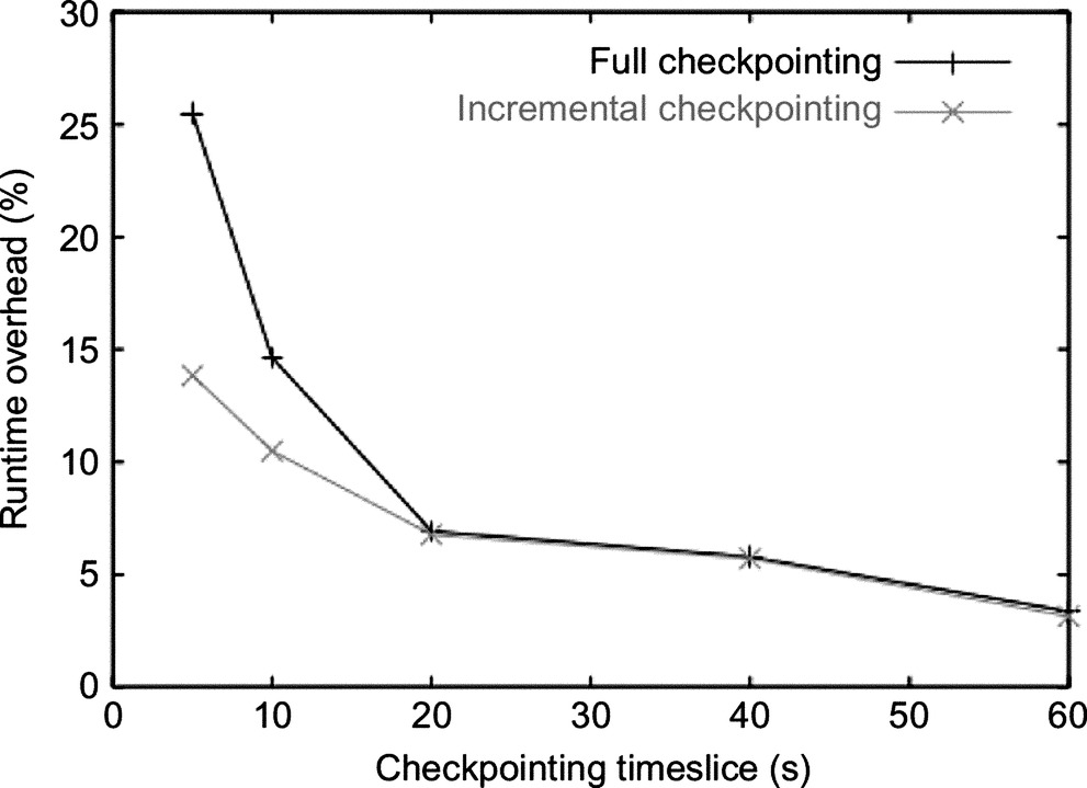
Fig. 5 shows the TICK runtime overhead for SAGE when using full and incremental checkpointing and saving the application state to disk. The plot shows that for small checkpointing intervals, incremental checkpoint is more efficient than full checkpointing, with a runtime overhead of 14% instead of 26% with a checkpointing interval of 5 s. However, as the size of the checkpointing interval increases, the relative advantage of incremental checkpoint decreases and eventually disappears with checkpointing intervals larger than 20 s. With such checkpointing intervals, in fact, the application rewrite most of its data structures, thus the number of dirty pages to be save in each incremental checkpointing interval approximates the full set of pages. Fig. 6 shows that, indeed, the number of pages to be saved with incremental and full checkpoint is fairly similar with a checkpointing interval of 20 s.

An OS-level implementation also provides access to information that are not generally available in user-mode, such as anonymous and file memory mappings, pending signals and I/O transfers, and hardware state. This information can help restore the state of the system and to understand which data has been actually transferred to I/O. At every checkpointing interval, TICK also saves the state of the system (both hardware and OS). At restart time, TICK restore the state of the system as it was before the failure, hence avoiding that the application be fast-forwarded in time just to restore the correct hardware and software state.
Despite their efficiency, OS-level implementations are not widely common, mainly because of the difficulty in porting and maintaining code among various OSs and even among different versions of the same OS. Virtual machines (VM) solutions have been proposed as an easier and more portable way to provide supervisor privileges to checkpoint/restart solutions. The general idea is that the application runs within a VM rather than directly on the host compute node. The VMM periodically saves the entire state of the VM on safe storage. For checkpoint/restart, the VMM leverage VM migration functionalities usually present in modern VMM to migrate VMs from one compute node to another in data-center installation. Upon restart, the checkpointed VM is migrated to an available compute node and restarted. Since there interaction between VM and host node is managed by the VMM and the guest OS is not aware of the actual hardware on top of which the VM is running, restarting a VM is a pretty seamless procedure.
Although privileged-level solutions provide easy access to system software and hardware information and provide faster restart, they incur in larger checkpoint sizes and increased consistency complexity. Privileged-level solutions do not reason in terms of data structures, but rather manage memory pages. A page is considered dirty even if a single byte in the page has been modified since the last checkpoint. Saving the entire page even for a minimal modification could results in an unnecessary space overhead. On the other hand, as discussed earlier for incremental checkpointing, parallel applications tend to rewrite their address space fairly quickly. If the checkpointing interval is large enough, there are good chances that most of the data contained in a page has been updated since the last checkpoint.
4 Application-Specific Fault Tolerance Techniques
System-level resilience techniques attempt to provide transparent solutions to guarantee the correct execution of parallel applications. Although general, these solutions may incur in extra-overhead caused by the lack of knowledge regarding the application’s algorithm and data structures. For example, full-checkpoint/restart systems save the state of the application without distinguishing between temporal and permanent data. As such, system-level techniques may save more data that it is actually necessary. In contrast, application-specific resilience and fault-tolerance solutions (also called application-based fault tolerance) leverage application knowledge and internal information to selectively protect or save data structures that contain the fundamental application state. Many scientific application’s algorithms have mathematical invariant properties that can be leveraged to understand the correctness of partial solutions. For example, the user could assert that a certain quantity be positive, thus errors are easily detectable if the sign of the quantity turns negative. In other cases, redundant information can be added to detect or detect/correct a finite number of faults.
On the positive side, application-specific resilience techniques generally introduce lower runtime and space overhead, are highly portable because they do not depend on the underlying architecture, and are generally more salable. Computing the residual error falls into the application-specific resilience techniques category, among the error detection solutions. The major drawback of application-specific techniques is the high-effort of maintainability and the lower productivity. Compared to system-level solutions, application-specific techniques have to be implemented for each algorithm and algorithm’s variant, as they are generally part of the application itself. Moreover, modifications to the algorithm (e.g., changing the solver of a linear algebra system) may require a reimplementation of the resilience part as well, as the original algorithm may have different mathematical properties.
Fortunately, many applications use fundamental operations that can be embedded in mathematical libraries together with their corresponding resilience solutions. One of such algorithm is the matrix-matrix multiplication used in many scientific codes. Let An, m be a n-by-m matrix and Bm, n be a m-by-n matrix. The result of multiplying A by B is a matrix Cn, n = An, m × Bn, m. In this case, the problem is determining whether matrix Cn, n is correct, given that the input matrices An, m and Bn, m are correct, and possibly correcting errors due to bit-flips. Check-summing is a well-know techniques used to guarantee the integrity of data in scientific computations, communication and data analytic, among others.
Check-summing techniques are based on adding redundant information to the original data. Once the computation is completed, the redundant information is used to determine the correctness of the results, in this case the matrix C. Let’s consider a generic matrix An, m:

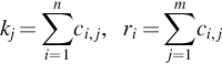
The column checksum matrix Ac of matrix A is an (n + 1)-by-m matrix which consists of matrix A’s first n rows plus an additional (n+1)th row that contains column-wise sums of the A’s elements. The elements of the additional row are defined as:

Similarly, the row checksum matrix Ar of matrix A is a n-by-(m + 1 matrix, which consists of the first m columns of A and a row followed by a (m+1)th column containing the sum of each row. The elements of Ar are defined as:
Finally, the full checksum matrix Af of matrix A is an (n + 1)-by-(m + 1) matrix composed by the column checksum matrix Ac and the row checksum matrix Ar and whose elements are defined as:

Ac and Ar can also be expressed as:

thus,

The computation of the original matrix C is extended to account for the redundant checksum information. In the case of C = A × B, the column checksum matrix Ac and the row checksum matrix Br are used to compute full checksum matrix Cf:

Obviously, computing Cf requires extra operations as compared to computing the original matrix C. In this case, thus, resilience is achieved through lower performance and higher energy consumption. The redundant information in Cf can be used to assess the correctness of C. More in details, the column and row checksum of the computed matrix C can be compared to the ones produces by multiplying Ac and Br. Let kj and ri be the column and row checksum of matrix C, respectively, such that:
then, kj and ri can be compared to cn+1, j and ci, m+1, respectively, to detect errors in each column j or row i, respectively. In this particular case, one single-bit error per column or row can be detected. If we assume that one error occurred during the computation, then the error can be located at the intersection between the inconsistent column j* and inconsistent row r*. With this technique, a single error can also be corrected by adding the difference between the checksum computed during the computation of Cf and the ones computed after the computation, kj and ri.
Although checksum is a fairly well-know and wide-spread solution, many other application-specific techniques have been developed for scientific algorithms [22–27].
5 Resilience for Exascale Supercomputers
HPC systems have historically been vulnerable to hard errors caused by the extremely large number of system components. Mechanical parts, such as storage disks, and memory DIMM failures were, and still are, among the most common reasons for system shutdown and require manual intervention or replacement. While this is still true in current-generation supercomputers and expected to worsen for future exascale systems because of the even larger number of system components, the stringent power constrains expected in the exascale era will change the balance between hard and soft errors. New low-power and near-threshold voltage (NTV) technologies, along with higher temperature and voltage tolerance techniques, are expected to be deployed on exascale system to address the power challenge [28]. Without additional mitigation actions, these factors, combined with the sheer number of components, will considerably increase the number of faults experienced during the execution of parallel applications, thereby reducing the mean time to failure (MTTF) and the productivity of these systems. Two additional factors further complicate the exascale resilience problem. First, power constraints will limit the amount of energy and resources that can be dedicated to detect and correct errors, which will increase the number of undetected errors and silent data corruptions (SDCs) [29]. Second, transistor device aging effects will amplify the problem. Considering that supercomputers stay in production for about 5 years, aging effects can dramatically diminish the productivity and return of investment of large-scale installations. The net effect is that new resilience solutions will have to address a much larger problem with fewer resources.
To address the exascale resilience problem, it is expected that new radical solutions be developed. Such solutions are currently under investigation and are not yet ready for deployment. This section will list the desirable properties and the main challenges that exascale resilience solutions will have to address.
5.1 Checkpoint/Restart at Exascale
Global checkpoint/restart will be prohibitive for exascale systems because of both space and time complexity. Given the massive number of parallel processes and threads running on an exascale system, saving the entire or even the incremental state of each thread on safe storage would require a prohibitively large amount of disk space. Since the I/O subsystem is not expected to scale as much as the number of cores, saving the states of each thread on disk would create severe I/O bottlenecks and pressure on the filesystem and disks. The serialization in the I/O subsystem, together with the large I/O transfer time necessary to save all thread states, will also increase the checkpoint time. Projections show that the checkpointing time might closely match or exceed the checkpointing interval, for representative HPC applications, thus the application may spend more time taking checkpoints than performing computation.
The second, but not less important, problem is how to guarantee checkpoint consistency for an application that consists of hundreds millions threads. Waiting for all the threads to reach a consistency point might considerably reduce the system utilization and throughput. Moreover, researchers are looking at novel programming models that avoid the use of global barriers, natural consistency points, as they have been identified as a major scalability limiting factor. Reintroducing these barriers, in the form of checkpoint consistency points, would bring back the problem and is, thus, not desirable.
5.2 Flat I/O Bandwidth
Many parameters are expected to scale on the road to exascale. Table 2 shows the past, current, and expected typical values of the most important system parameters, including the core count, memory size, power consumption, and I/O bandwidth.4 Most of the system parameters see an increase, albeit not always linear, from petascale to exascale systems. For example, the total number of processor core increases from 225,000 in 2009, to 3 and 5 million in 2011 and 2015, and it is expected to be in the order of billion in exascale systems. The I/O bandwidth per compute node, on the other hand, remains practically flat. While the overall I/O bandwidth is expected to double from 2015 to 2018 and to reach about 20 TB/s, the number of compute nodes per system is expected to increase much more, hence the I/O bandwidth available per compute node may decrease. This means that, on one side the number of cores and process threads will increase by two or three orders of magnitude, while, on the other side, the I/O bandwidth used to transfer checkpoints from local memory to stable storage will remain constant or slightly decrease. Moving checkpoints to stable disk is one of the aspects of the exascale data movement problem [30]. With memory systems becoming more hierarchical and deeper and with the introduction of new memory technologies, such as nonvolatile RAM or 3D-stacked on-chip RAM, the amount of data moved among the memory hierarchy might increase to the point of dominating the computation performance. Moreover, the energy cost of moving data across the memory hierarchy, currently up to 40% of the total energy of executing a parallel application [30], may also become the primary contribution to the application energy profile.
Table 2
Past, Current, and Expected Supercomputer Main Parameters
| Systems | 2009 | 2011 | 2015 | 2018 |
| System peak FLOPS | 2 Peta | 20 Peta | 100–200 Peta | 1 Exa |
| System memory | 0.3 PB | 1 PB | 5 PB | 10 PB |
| Node performance | 125 GF | 200 GF | 400 GF | 1–10 TF |
| Node memory BW | 25 BG/s | 40 GB/s | 100 GB/s | 200–400 GB/s |
| Node concurrency | 12 | 32 | O(100) | O(1000) |
| Interconnect BW | 1.5 GB/s | 10 GB/s | 25 GB/s | 50 GB/s |
| System size (nodes) | 18,700 | 100,000 | 500,000 | O(million) |
| Total concurrency | 225,000 | 3 million | 50 million | O(billion) |
| Storage | 15 PB | 30 PB | 150 PB | 300 PB |
| I/O | 0.2 TB/s | 2 TB/s | 10 TB/s | 20 TB/s |
| MTTI | O(days) | O(days) | O(days) | O(1 day) |
| Power | 6 MW | 10 MW | 10 MW | 20 MW |

Considering the expected projections, extending current checkpointing solutions to exascale will considerably increase the pressure on data movement. New resilience solutions for exascale will necessarily need to reduce data movement, especially I/O transfers. Local and in-memory checkpointing are possible solutions, especially for systems that features nonvolatile memory (NVRAM) [31]. In this scenario, uncoordinated checkpoints are saved to local NVRAM. In case of failure, the failed compute node will restart and resume its state from the checkpoint store in the local NVRAM memory, while the other nodes will either wait at a consistency point or restore their status at a time before the failure occurred. This solution has its own limitations: First, if the failed node cannot be restarted, the local checkpoint is lost. To avoid such situations, the each local checkpoint can be saved to remote, safe storage with a time interval much larger than the local checkpointing interval. Second, the checkpoint/restart system needs to guarantee consistency when recovering the application. As explained in the next section, novel parallel programming models might help to alleviate the need of full consistency across the application treads.
5.3 Task-Based Programming Models
Synchronizing billions of threads through global barriers might severely limit the scalability of HPC applications on future exascale systems and the system productivity. Novel programming models are emerging, which provide asynchronous synchronization among subset of application threads, generally much smaller than the total number of threads. Task-based programming models are among the most promising programming models for exascale systems [32–34]. Task-based programming models follow a divide-and-conquer approach in which the problem is decomposed in several subproblems recursively until a small unit of work (task) is identified. The efficacy of task-based approaches is based on the idea of overprovision the system with a myriad of tasks that will be managed and assigned to worker threads by an intelligent runtime scheduler. The number of instantiated tasks is much larger than the available computing units, i.e., CPU and GPU cores, so that there are usually tasks available to run on idle cores. The runtime scheduler takes care of mapping a task to a computing element.
Fig. 7 shows a possible task-based implementation of the Fibonacci algorithm. The program in Fig. 7A follows a fork-join semantics in which tasks are spawn at each level of the recursion and synchronize after completing their computation. The When a task spawns another task (fork point), the runtime scheduler decides whether the current worker thread will execute the newly spawn tasks (blue nodes in Fig. 7B) or their continuation (yellow nodes in Fig. 7B). The suspended task or continuation will be placed on a local stack. Idle worker threads will be able to steal from busy worker threads’ stacks thereby providing automatic load balancing. After completing their computation, each task will reach a synchronization point (gray nodes in Fig. 7B). Only after all the spawn tasks reach the synchronization point, a task can continue its computation. The synchronization points (or join point), thus, act as local barriers.
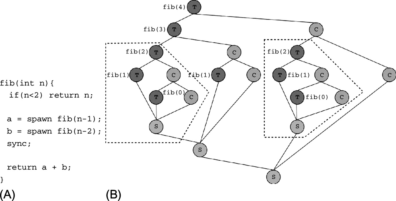
Task-based programming models are attractive for two main reasons: their adaptivity and the decoupling of computation and data. The adaptive and dynamic nature of the task-based approach allows for adapting the computation to a given set of computing resource whose availability varies in time and for performing automatic load balancing. One of the possible causes that may reduce the amount of computing resources available is the occurrence of failures. In case of failure, the work performed by the failed node can be re-executed by another node without forcing all the other compute nodes to roll-back to a previous checkpoint. For example, if the compute nodes that executed the tasks within red, dashed lines in Fig. 7B fail, other compute nodes can re-execute the lost computation without rolling back the other live worker threads.
Dividing the execution of an application in tasks also provides an inherent form of soft errors containment. In fact, if a fault is detected before a new task is spawn and if the current task as only modified local variables or local copies of variables, it is possible to re-execute only the current task without even notifying the other worker threads of the detected failure. This model is particularly suitable for data-flow programming models, in which tasks exchange data only through input and output parameters. In case tasks also modify global data structure, it might still be required to perform a form of checkpointing. However, since task-based programming models decouple computation and data structure, it is possible to restart the computation with a different set of worker threads without explicitly redistributing data. This means that the checkpoint consistency does not need to be guaranteed for all worker threads in the systems but only for the ones that are somehow impacted by the failure, i.e., the worker threads that spawn the failed tasks. This greatly reduces the complexity of taking checkpoint and avoid the use of global barriers as synchronization points.
5.4 Performance Anomalies
An interesting new dimension for exascale systems is represented by the fact that hardware components gracefully degrade performance in the presence of contingent problems or because of aging. This behavior are not necessarily caused by hardware faults but are still considered performance anomalies and undesirable. For example, a processor core may reduce the operating frequency if the temperature raises over the safe threshold. Similarly, a network links may reduce the transferring bandwidth if the number of packets corrupted reduces the quality of service. In these cases the system continues to operate “correctly” but the performance provided does not match the expectation of the users. Although these examples are not generally considered under the scope of resilience techniques, the symptoms they expose are often similar to the ones generated by hard and soft errors. Moreover, the effects of these performance faults can be assimilated to the PEX cases analyzed in Section 2. It is thus necessary to distinguish performance anomalies caused by hard or soft errors from those caused by contingent conditions. In most cases, it is frustrating to see that an application does not perform as expected even if everything looks OK and performances of previous runs, in the “exact same conditions,” were higher.
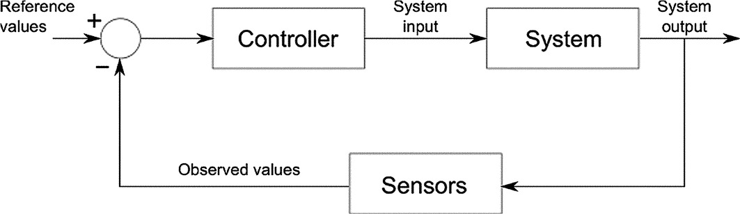
To be able to disambiguate actual hardware faults from performance anomalies or, more in general, be able to understand whether the performance provided by an application in a particular run are satisfactory, researchers have proposed lightweight runtime monitoring that analyze the performance of a parallel application and compare current performance against previous executions or application performance models. In case a discrepancy between observed and expected performance or in case a fault is detected, the monitor may activate a controller module that will take the necessary actions to guarantee the correct and satisfactory execution of the application. Fig. 8 shows a graphical representation of how monitor, controller and applications are placed in a closed feedback loop.
The feedback system depicted in Fig. 8 can be used to detect performance anomalies caused by the thermal management system, which may reduce the processor frequency or skip processor cycles to reduce the temperature of the system. Fig. 9 shows the outcome of this test case: the plot reports the performance in FLOPS of NEKBone during the execution of the application. NEKBone is a thermal hydraulic proxy application developed by the ASCR CESAR Exascale Co-Design Center to capture the basic structure of NEK5000, a high order, incompressible Navier-Stokes solver based on the spectral element method.5 NEK5000 is an MPI-based code written in Fortran and C that employs efficient multilevel iterative solvers and designed for large eddy simulation (LES) and direct numerical simulation (DNS) of turbolence in complex domains. NEKBone mimics the computationally intense linear solvers that accounts for a large percentage of the more complicated NEK5000 computation, and the communication costs required for nearest-neighbor data exchange and vector reduction. In particular, the NEKBone kernel solves a standard 3D Poisson equation using the spectral element method with an iterative conjugate gradient solver with an orthogonal scaling preconditioner.

From the plot it is evident how some processor cycles are periodically skipped and the application performance decreases. A monitoring system can detect the sudden lost of performance and activate the controller, which can identify the reason behind the performance drop (e.g., high temperature) and take the proper corrective actions to maintain satisfactory performance and lower the temperature.
Although the example in Fig. 9 is just a test case, it highlights a general trend for exascale systems. Given the extreme level of parallelism, the large number of system components, the thigh power budget, and the high probability of soft and hard fault, exascale systems will be dynamic and applications will be forced to run in changing execution environments. Self-aware/self-adaptive systems become essential to be able to run in such environment and still obtain the desired performance and correctness while maintaining the target power budget.
6 Conclusions
Although not generally deployed in hostile or unsafe environments, supercomputers have historically be particularly susceptible to soft and hard faults because of their extremely large number of system components, the general complexity of these systems, and the environmental conditions in which they operate. Without appropriate resilience solutions, it would be impractical to run a large-scale application on modern supercomputers without incurring in some form or errors.
Many fault-tolerance solutions have been developed throughout the past years. Some of these solutions, such as checkpoint/restart, are transparent to the user and can be employed with different application without or with minimal code modification. Other solutions are more intrusive and strongly depends on the mathematical characteristics of a particular algorithm or algorithm’s implementation. Such application-level solution allow the user to specify which data structures are essential for the correct recovery of the application in case of failure and which are only temporal.
As systems become larger and include more components, the probability of failures increases. Moreover, the strict power limits enforced on exascale systems will force the use of novel low-power and NTV technologies, which, together with the massive number of system components, will negatively impact system resilience. Projections show that the number of soft error that may result in SDC will become dominant in the exascale era and that novel resilience solutions are necessary to guarantee the correct execution of HPC applications.
Current solutions based on global checkpoint seem impractical at the scale of future generation supercomputers, both because of the limited I/O bandwidth and because of the difficulties in guaranteeing consistency upon restart. Novel programming models, such as task-based programming models, are emerging as new programming models for exascale systems. These new programming models incorporate, directly or indirectly, primitives or properties that can be leverage to increase system resilience to the point that is needed by exascale supercomputers.