4

Leveraging Lean Flow to Keep the Work Moving

In Chapter 1, Introducing SAFe® and DevOps, we saw the inclusion of Lean thinking approaches such as Lean software development and Kanban into the Agile movement. Jez Humble saw it as important enough to include it in the CAMS model, creating the CALMS model from which we base the SAFe® CALMR model. Scaled Agile talks about that Lean-Agile mindset with an emphasis on both Lean thinking and an Agile mindset derived from the Agile Manifesto. How does this focus on Lean thinking manifest itself in DevOps and SAFe?

In this chapter, we will see that keeping product development moving at a predictable pace requires the establishment of a Lean flow. Proper flow allows automation to succeed. To that end, we will look at the following practices to establish Lean flow:

• Making sure all work and work progress is visible
• Limiting our Work in Progress/Process (WIP)
• Keeping the size of each batch of work appropriately small
• Monitoring our work queues
• Employing systems thinking to change the traditional definitions of project and teams

Making the work visible

Work could be defined as the effort the team or Agile Release Train (ART) (as a team of teams) may put forth to develop a product or solution. But not all that work may be focused on customer value.

The Phoenix Project: A Novel about IT, DevOps, and Helping your Business Win by Gene Kim, Kevin Behr, and George Spafford identifies four kinds of work. These are summarized as follows:

• Business projects: Requests for new features that will bring value to the customer
• Internal projects: Work that helps organizations continue to develop products efficiently
• Maintenance: Work needed to maintain existing products
• Unplanned work: Bugs, defects, and emergencies that occur from time to time

SAFe takes a few of these work categories and places them in enablers. The idea here is that enablers help create future business value. The four kinds of enablers defined by SAFe are listed here:

• Infrastructure: This enabler exists to enhance how products can be developed and delivered. Examples include new automated tests to include in the continuous delivery (CD) pipeline.
• Architectural: This enabler exists to enhance the architecture that business features and user stories rely on. SAFe defines the sequence of architectural enablers as an architectural runway that drives future business value. Examples include creating a new database server virtual machine (VM) for the staging and production environments.
• Compliance: This enabler describes additional work that may be needed in certain regulated industries. Examples include Verification and Validation (V&V), approvals, and documentation.
• Exploration: Sometimes, additional research is required to understand the optimal approach, learn about new technologies, or refine customer desires. Exploration enablers are created to identify the work that research requires. An example of this is a Spike, used by Agile teams to research new technologies or evaluate a development option, such as determining the correct technology for web streaming.

Given the different categories of work that is done, it’s important to have a uniform way of displaying all the work of a team or ART. Traditionally, enterprising people, often with a technical background, have resorted to spreadsheets whose arrangement is flexible to allow for additional information such as work category or status. In addition, sharing spreadsheets among team members becomes difficult as there may be changes that need to be synchronized.

Dominica DeGrandis, in her book Making Work Visible, Exposing Time Theft to Optimize Work & Flow, notes that the majority of people are visual-spatial learners, in that they are able to understand and respond to information presented visually. This is one of the reasons for setting up a Kanban board.

A Kanban board is a space divided into columns. Each column represents a state in the workflow of an item of work. Items of work are represented by note cards and color-coded to represent the appropriate work category.

A simple Kanban board is illustrated in Figure 4.1. Note the three columns, representing work to be done (Backlog), WIP (Doing), and work completed (Done):

Figure 4.1 – Simple Kanban board

Additional features on a Kanban board can help teams manage the work they do. Let’s take a look at those other features on a Kanban board.

Specifying workflow with additional columns

Often, having a single in-progress column doesn’t provide visibility into everything that a team or ART is doing, especially if there are bottlenecks in the overall process. It makes sense to break up the in-progress column to highlight major steps in the development so that bottlenecks are easy to identify.

While having discrete process steps separated into separate WIP columns is generally done, it’s important to remember that teams shouldn’t be taking all issues and moving all of them from column to column as that devolves the process into Waterfall. The movement of the issues happens in a continuous fashion.

Figure 4.2 shows an illustration of separating our Doing column with stages for analysis, implementation, and review:

Figure 4.2 – Expansion of the Doing column into several stages

Flagging impediments and urgent issues

Sometimes a work issue may be blocked due to some external event or dependency. As these impediments or blockers come up, an icon can be attached to the work issue as an indicator to the teams to continue to pay attention to the issue until the blocker is removed.

In the same way, any urgent issue may need the attention of the entire team. The team may need to swarm on the urgent issue until it is resolved. Urgent issues may be identified by a special indicator put on the issue or by its position in an expedite swimlane that cuts horizontally across all columns of the Kanban board. In the following screenshot, an example of an urgent issue highlighted by a special indicator in the expedite lane is illustrated:

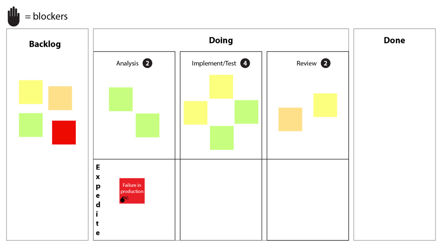
Figure 4.3 – Work issue with an urgent indicator in the expedite lane

Policies for specifying exit criteria

For every stage in the process, the team needs to have a clear agreement on the exit criteria. Having clear exit criteria avoids confusion as to whether an issue is truly finished at that stage. This agreement for each column is known as a policy.

Column policies have their place in a team charter or working agreement so that these are explicit and agreed upon. Examples of this include a Definition of Ready (DoR), where any questions are answered, and requirements are detailed enough that development can begin. Another example is a Definition of Done (DoD), which is an agreement by the team of the criteria that determine when a story is complete and development work on that story can stop. These policies avoid any confusion about whether a piece of work is truly complete as opposed to done done.

Other additions to the Kanban board will be identified as we look at other practices to ensure that Lean flow occurs. In the following section, we will examine the problem of having too much WIP and how a Kanban board can help by providing visibility and enforcing constraints on team behavior.

Limiting WIP

WIP is the work a team or ART has in process. It has been started but is not complete. If we were to view WIP on our Kanban board, it would resemble the following screenshot:

Figure 4.4 – Kanban board highlighting WIP

It is important to make sure that the work within these columns is monitored so that it doesn’t overwhelm the teams or ART. According to Dominica DeGrandis, the effects of too much WIP may include the following:

• Too much multitasking, which will cause teams to spend too much time doing context switching and prevent them from finishing work
• New work items are started before existing work is finished
• Work takes a long time to finish (long lead times/cycle times)

A key way of ensuring that a team is not letting WIP go unchecked is by setting up WIP limits or constraints on each column between the Backlog column (where work has not been accepted yet) and the Done column (where completed work goes). An example of WIP limits on a Kanban board is shown in the following screenshot:

Figure 4.5 – WIP limits on columns

To understand how WIP limits can help a team achieve Lean flow, consider the following comparison of team behavior.

First, imagine a Kanban board with no WIP limits. A developer on the team has just finished the development of a user story. It meets the policy criteria for the column and could be pulled to the next column. If the developer moves that story to the next column and pulls a story to work, has that developer done anything to lower the amount of work that’s in progress? This may be acceptable if there is flow already established, but if there is a bottleneck in the team’s process, this action may exacerbate the bottleneck and prevent the entire team from actually delivering. This situation is captured on our Kanban board in the following screenshot:

Figure 4.6 – Scenario with no WIP limits, resulting in no reduction in WIP

Now, let’s imagine the same Kanban board with WIP limits in place. That developer who has finished the user story cannot move anything into the Implement/Test column. Also, no one can move anything from Implement/Test into Review. To help get the bottlenecks fixed, the developer acts to assist other team members to move a story from Review to Done. This has the effect of introducing throughput and establishing flow. We can view this scenario in the following screenshot:

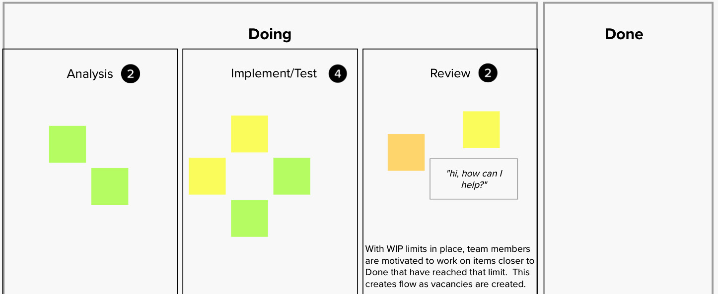
Figure 4.7 – Scenario with WIP limits, resulting in flow

Teams can select initial WIP limits as they start work. After a period of time, if bottlenecks are still seen, they can lower the WIP limits until the bottlenecks disappear, and flow at that point is achieved. Even with that bottleneck gone, other bottlenecks will appear. The Theory of Constraints, as written by Eliyahu M. Goldratt in his book The Goal, specifies that you move to the subsequent bottlenecks, removing them one by one, to optimize the flow for the entire process.

WIP limits are a necessary mechanism according to David J. Anderson in his book Kanban: Successful Evolutionary Change for Your Technology Business. WIP limits create tension for a team, encouraging the team to act in order to work and enable flow, as seen in our previous scenario. The tension also may highlight constraints and systemic impediments in the organization. Open discussion of these constraints and impediments to finding solutions leads to continuous improvement.

We’ve seen how limiting WIP by imposing column constraints or WIP limits may help us address bottlenecks in our development process. One other source of bottlenecks in our process is the size of our items of work. Let’s take a look at keeping those at an appropriate size to attain and maintain flow.

Keeping batch sizes small

Batch size commonly refers to the size of a standard unit of work. One of the accomplishments of the Agile movement was the success of focusing delivery on smaller increments. That forced a look at reducing the batch size that could be accomplished for delivery. Reducing batch sizes in addition to limiting WIP are important parts of accomplishing Lean flow. Donald Reinertsen noted the effects of batch size in his book The Principles of Product Development Flow: Second Generation Lean Product Development. Let’s examine what role small batch sizes play.

Small batch sizes decrease cycle time

A key takeaway from Agile development was the delivery of value in short cycles. This had the effect of shortening the cycle time a team had to deliver an increment of value, allowing the team to look at delivering only what it could deliver by the end of the cycle. This allows us to say that batch size is directly related to the cycle time.

Keeping to large batches of work has several adverse effects. The work may not be delivered by the end of the cycle. What may be delivered may have defects that need to be fixed or reworked, increasing cycle time. The appearance of these defects also increases batch sizes, creating a snowball effect. The growth of the batch size and cycle time leads to cost overruns and schedule slippages.

Small batch sizes decrease risk

As we saw in the previous subsection, a large batch of work may carry with it defects that need to be fixed, impacting both the overall batch size and cycle time. Working in small batches will not eliminate the possibility of defects but will keep the number of possible defects small so that they can be managed easily.

A side effect of small batch sizes is that they result in short cycle times. This short cycle time provides opportunities for customer feedback. The opportunity for feedback negates any risk that the team is moving in the wrong direction in terms of delivering value.

Small batch sizes limit WIP

Batch sizes and WIP are directly related to each other. Directly changing one changes the other in a correlated fashion. Let’s look at a few examples of this correlation at work.

A large batch size will mean there is a large number of items of WIP. As mentioned before, large numbers of WIP increase multitasking, preventing work from finishing because of increased context switching. This effect is another factor that increases cycle time.

The large batch size also creates a bottleneck in the system. This variability in flow impedes work from effectively moving, increasing cycle time.

Reinertsen also advocates in his book The Principles of Product Development Flow: Second Generation Lean Product Development that when optimizing between batch sizes and limiting WIP by attacking bottlenecks, start with reducing batch sizes first. This is often an easier step to implement. Reducing bottlenecks to allow for adequate flow may involve deeper changes in both process and technology.

Small batch sizes improve performance

As counter-intuitive as it may seem, large batch sizes do not create efficiencies with overhead. Time processing overhead activities are actually greater with large batches as opposed to smaller batches. The overhead compounds on large batches. Overhead costs on small batches can be reduced easily because of the shorter cycle times.

Small batch sizes improve efficiency. This may seem to also be counter-intuitive, but because small batch sizes receive fast feedback, subsequent batches of work are able to take advantage of that feedback, reducing rework. A large batch of work exposes all those problems at once, creating more work and removing any implied efficiency.

We’ve seen the advantages of working with small batch sizes and what happens when you work with a large batch size. The question then becomes, “How do I make sure I’m not working with a large batch size?” Let’s take a look at finding out what your optimal batch size is.

Finding the ideal batch size

We have identified the benefits of working with small batch sizes. The question then becomes, “What would be an adequate enough batch size?”

Reinertsen proposes looking at batch size in terms of economics. When approaching the cost of development and determining what size of work is ideal, you need to consider two costs:

• Holding cost: The cost of keeping (and not releasing) what you develop
• Transaction cost: The cost to develop your work

An example of this comes from releasing work to a production environment. The following diagram shows the relationship between the transaction and holding cost curves if we were to look at the cost of releasing a change versus the cost of waiting to collect changes at an optimal time:

Figure 4.8 – Transaction and holding cost curves

In our preceding diagram, an example of a small change—such as a single line of software code to release—is represented by point A. At point A, we incur a very low holding cost to immediately release, but the high cost at point A comes from the transaction cost. We are spending a lot of time performing testing and deployment for a simple line of code.

Does this mean we should always look to consolidate changes to incur less cost? Let’s look at point B in our preceding diagram, which collects our changes over a larger time period—say, a month. Now, the costs are reversed. The transaction cost is low as we are performing testing and releasing a large number of changes, but now our holding cost is high. Perhaps in delaying the release of our change, we missed an important market window and lost sales because our competitors released an equivalent change first.

If we wanted to figure out the break-even point of when to actually release a collection of changes, we would perform a u-curve optimization. We would take the sum of the holding cost and the transaction cost and plot it on the same graph as shown in the preceding diagram. On the graph of the total cost curve (sum of holding cost and transaction cost), find the lowest point on the curve. That’s the ideal number of items to have in your batch.

How can we improve on this ideal number of items per batch? If we introduce new ways of doing things or new technology, that can affect the transaction cost, giving us a new total cost curve with which to perform a u-curve optimization. Extending our example of releasing changes into production, the use of automated testing and deployment tools that enable faster, more reliable deployments with more frequent testing in a CD pipeline reduces transaction costs, giving us the confidence to release stories more frequently within a sprint. The new cost curves would probably resemble the following diagram:

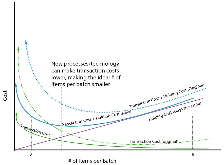
Figure 4.9 – New cost curves after optimization

We can see from the preceding diagram at point A, the holding cost remains the same but the transaction cost has decreased. Also, we can see that the low point of the total cost curve has shifted to the left, moving our ideal point “left," to smaller batch sizes.

So, what can our teams and ARTs do that will yield lower transaction cost curves? Adopting practices and technology such as automated testing and automated deployment is one example that certainly fits the bill. They allow for smaller batch sizes to go through and encourage flow.

In this section and the previous section, we looked at WIP and batch size as factors for achieving Lean flow. In the next section, we will see how those factors work with other factors to determine whether your system has Lean flow.

Monitoring queues

To enable Lean flow, you need to closely examine queueing theory, the mathematical field behind the behavior of queues and waiting in line (think Starbucks or the checkout area of your local supermarket!). A number of mathematical formulas will be useful in helping us make sure we understand what we have to do to ensure Lean flow. These are:

• Little’s Law
• Kingman’s Formula

Let’s see how we can use these elements of queueing theory to enable Lean flow.

Where are our queues?

A key difference between product development queues and product manufacturing queues is that the artifacts of product development (particularly software development) are not physical and it is difficult to grasp the progress until completion, whereas in manufacturing, you can visually ascertain the completeness of a product while on the factory floor. This invisibility factor makes it easy to ignore these queues, often at your own peril.

Long queues unrestrained by WIP limits or small batch sizes create an array of problems, as summarized by Reinertsen. These problems include the following:

• Longer cycle times
• More risk
• More overhead
• More variability
• Lower quality
• Lower motivation

We’ve talked about problems with overhead, risk, and quality when talking about large batch sizes. If we consider the size of our work as the queue for our system, then the mathematical formulas that we will examine later are applicable and can model the state of our Lean flow.

How can long queues lower workplace motivation? Imagine a scenario where you were preparing work and the next part of the process was ready whenever you finished it. There would be a sense of urgency to finish your part of the work. That sense of urgency would not be there if, after you delivered your work, it sat behind a queue of other items and wouldn’t be seen for weeks.

Now that we’ve established our batch sizes and WIP as queues, it’s time to see how mathematical formulas illustrate the relationship between our queues and cycle time and variability.

Little’s Law and cycle time

We have seen how both WIP and batch size correlate to cycle time, or the time it takes to deliver work once we’ve accepted it. Mathematically, cycle time, WIP, and batch size are tied using Little’s Law.

Little’s Law is an expression tying cycle time, WIP or batch size, and throughput. This expression for Little’s Law is presented here:

L stands for the length of the queue. This can be thought of as either WIP or batch size. L is the throughput of work processed by the teams or ART. W gives you the cycle time or the wait time for a customer.

At this point, it’s simple mathematics if we’re concerned about finding out our cycle time. Written in the following manner, you can see that cycle time (W) is directly related to the size of our queue (L):

A simple illustration of this is a backlog for a Scrum team. If their backlog has 9 user stories, each estimated at 5 story points, and their velocity (the measure of how many story points’ worth of work they have been able to deliver per sprint) is 15 story points per sprint, we can take Little’s Law to predict how many sprints it will take to complete that set of stories in the backlog, as illustrated in the following diagram:

Figure 4.10 – Illustration of Little’s Law

Kingman’s Formula

Kingman’s Formula is a mathematical model to describe how wait time equates to cycle time, variability, and utilization. The formula is illustrated here:

Each term in the formula represents an individual quantity. The first term represents the utilization of the people doing the work. The second term () represents the variability of the system. The third term (t) represents the service time or the cycle time.

We want to examine the relationship between wait time, utilization, variability, and cycle time. If we substitute a letter for each term, we get the following (simpler) equation, commonly referred to as the VUT equation:

So, this equation shows us that the total wait time for a customer is directly proportional to the utilization, variability, and cycle time.

We have previously looked at how queue size, batch sizes, and limiting WIP have an effect on cycle time. Let’s take a look at the other variables of Kingman’s Formula to see how utilization and variability can affect the wait time.

Utilization and its effects

Let’s start with utilization. When we refer to utilization, we look at the percentage of the overall capacity of the system. A high utilization may be desired by management—after all, we don’t want our workers to goof off. But after looking at Kingman’s Formula, we see that wait time increases as utilization increases. We can see this effect by plotting out utilization in comparison to the queue size. The resulting curve is a nonlinear graph that starts to ascend around 60% utilization and approaches infinity at 100% utilization. This is seen in the following diagram:

Figure 4.11 – Utilization compared to queue size

Another way of looking at this percentage utilization is seeing it as a load/capacity. If load looks at the rate at which new work comes in, capacity looks at the rate at which work leaves and is delivered to the customer. This ensures adequate utilization so that we do not take in more work than we can process.

The idea that for Lean flow to occur, scheduling slack or idle time must be introduced to keep utilization at a reasonable level (for example, not at 100%) has its roots in the Toyota Production System. Muri or overburdening was seen as one of the three wastes to eliminate in Lean. We will look at another waste: Mura, or unevenness. We also call this variability.

Variability, its effects, and actions

Let’s explain what variability is. So far, we’ve been making the assumption that, as with manufacturing products on a factory floor, all work involves the same effort. But this is often not the case. Each piece of work may involve different levels of effort or even different efforts. Some work may have unknowns that require a more detailed investigation. Some work may have defects. Variability is the quality that describes the individuality of each piece of work.

From Kingman’s Formula, we see that the effects of variability have a compounding effect on wait time. The curve in the following diagram shows the effects of high variability versus low variability when looking at utilization:

Figure 4.12 – Effects of variability on utilization and queue size

We can see from the preceding diagram that this effect is linear, but the combination produces an undesired result. With high variability, working at somewhat lower utilization will not stem the growth of your queue. You’d have to work at much lower utilization to keep your queue in control. What can you do?

It’s important to understand that not all variability is bad. Some may be necessary to learn new things. So, the key is really to manage variability so that it doesn’t affect the queue size and, consequently, the wait time. Ways to do that include the following:

• Limiting WIP
• Working with smaller batch sizes
• Setting up buffers in your system
• Establishing standard processes

We’ve spoken before about the benefits of limiting WIP and working with smaller batch sizes, so let’s examine some of the other ways we can manage variability.

Setting up process buffers

Lean manufacturing looks to limit variability by setting up buffers. These buffers are used to limit the following factors:

• Inventory
• Capacity
• Time

In product development, WIP limits and small batch sizes act as inventory and capacity buffers accordingly. To set up a time buffer, you can establish buffer states on those WIP columns on your Kanban board where variability exists in your process. An example on our Kanban board is shown in the following screenshot:

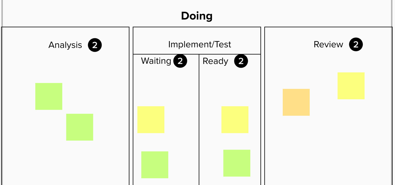
Figure 4.13 – Kanban board with buffer states in the Implement/Test column

Note that WIP limits are established in each buffer state to ensure throughput is maintained.

Establishing standard processes

In the previous section, we discussed using several types of buffers to ensure that variability is managed at several stages of the process. The variability managed by buffers is often the type that is tolerated, even encouraged by the nature of the work.

Some variability, however, may exist due to inefficiencies in the development process. An example of this is encouraging one type of test to be automated—for example, unit tests for code—without striving to automate behavior-driven development (BDD) tests to ensure correctness. This has the effect of keeping cycle times long.

Establishing standard processes ensures the reduction of needless variability of cycle time. Standardizing processes includes establishing a standard, detecting any possible problems, and discovering the root cause of these problems continuously.

We’ve seen the practices you can use to model your development process to ensure that the work is progressing to completion. These practices need to be anchored by people that look at the entire process from start to finish. In the next section, we’ll take a closer look at establishing that viewpoint and the systemic changes needed.

Moving from project-based to product-based work

When adopting value stream thinking, it’s important to change the view and mindset of development from project-based management to product-based management.

In Project to Product: How to Survive and Thrive in the Age of Digital Disruption with the Flow Framework, Mik Kersten contrasts the success of integrating IT and software in assembling BMW models in Leipzig, Germany, with the failure of Nokia to continue its dominance in the smartphone industry as the iPhone and Android phones were introduced. He notes that although Nokia had successfully adopted Agile practices, it did not appear to foster change to the entire product development process or affect the entire organization. He identifies that for this Age of Software, product-oriented development using value streams allows for the creation and maintenance of successful products.

Mik Kersten highlights seven key categories where the differences between project-based management and product-based management are apparent. These differences are illustrated as follows:

• Budgeting
• Timeframe
• Success
• Risk
• Team assignments
• Prioritization
• Visibility

Let’s individually look at these differences now.

Project budgets versus value stream funding

In project management, the iron triangle is a well-known construct. In management, you look at three factors or sides to see whether you can fix one or more of them to bring a project or product to completion. These three factors are as follows:

• Resources (people, equipment, facilities, and so on)
• Scope
• Time

A project budget is often a bet. Can the project do everything required (scope) in the projected timeframe (time) and with the projected resources? Because this budget is necessary for approvals, it is often a guess of the largest number of resources for the other parts of the triangle. Sometimes these guesses fall short, resulting in cost overruns and possibly another project (with another budget).

Funding for value streams is easier. Resources and time are kept constant over the period of the budget. At the end of the timeframe for the budget (often less than an annual basis; typically, quarterly) the results of the development and the customer feedback determine whether continued effort and capacity are needed to match the demand for delivered features. If so, a new budget with an increased allocation is created for the new time period.

Defined endpoint versus product life cycle

A defining characteristic of the project is its life cycle There is a beginning, with a flurry of activity to organize teams and get started. This then proceeds along with development, continuing until the project reaches its conclusion: the delivery of a product. At this point, the project is over. With the project and its funding at an end, the teams that developed the product are dispersed. The product goes to a dedicated maintenance team that may not have had a role in its development, consequently preventing learning from reaching the entire organization.

Value streams approach the timeline of the entire product from cradle to grave. The same teams and ARTs that develop and release the initial features of a product become responsible for its maintenance and ongoing health. Part of maintenance includes identifying and removing technical debt, resulting in keeping the product viable. This occurs until the product reaches the end of its life.

Cost centers versus business outcomes

Measurement of progress in project-based development is often aligned with how the cost centers that comprise teams are performing. This disjointed view of progress focuses on the performance of individual silos rather than the entire system.

Another consequence of this cost-center approach is that because the budgets tend to be large, the project stakeholders are drawn to create large projects as opposed to viewing the value of efforts once delivered.

Value streams use a different metric for success. They look at the outcomes produced by efforts delivered. By allowing for incremental delivery and learning from customer feedback, the value stream can adjust to deliver better business outcomes.

Upfront risk identification versus spreading risks

In project-based development, risks to delivery are identified as early as possible to create contingencies. But frequently, there are risks not identified due to the unknowns yet to be discovered when development is underway.

With product-based development, risks are identified as more learning occurs. Incremental delivery allows for pivots to occur at regular checkpoints. Although there may be overhead involved in these pivots, this overhead is spread out over the product life cycle and becomes a small fraction as it is distributed over that long period of time.

Moving people to the work versus moving work to the people

Project-based development creates teams from cost-center-based resource pools. This method of creating teams to work on projects assumes that individuals from the resource pools have identical talents and skills. This assumption is never true.

Another consequence of this reallocation of these individuals interferes with the team’s well-being and productivity. In 1965, psychologist Bruce Tuckman created the Forming, Storming, Norming, Performing, and Adjourning (FSNPA) model of team creation, illustrating the stages teams go through as they become high-performing. Constant reassignments and team shakeups impede the ability of the team to achieve a high-performing status where the team works as one unit.

Product-based development emphasizes long lifespans for teams. This allows teams to focus on acquiring product knowledge and grow together as one team. This improves the ability of the team to deliver and the team’s morale.

Performing to plan versus learning

In project-based development, adherence to the project plan is paramount. Adjustments to the plan result in cost overruns and reallocation of resources due to the overhead cost of performing any changes.

Product-based development welcomes changes by setting up piecemeal delivery of features and creates a space for learning and the validation of hypotheses. After the delivery of each increment of value, feedback and outcomes are collected and necessary adjustments are made.

Misalignment versus transparent business objectives

In project-based development, there is often a disconnect between the business stakeholders and the IT departments that develop products. This disconnect stems from IT’s focus on the product and the business side’s focus on completing the project through a progression of steps with no runway for readjustment.

With product-based development, the goals for both the business and IT development sides are the same: the fulfillment of business objectives. This transparency of the goal allows for alignment to occur and for easier sharing of progress and feedback.

Summary

In this chapter, we looked at Lean flow as part of the CALMR model. We know that achieving a Lean flow of work where the progression of work is steady and teams are neither overburdened nor underburdened allows for the success of the other parts of the model. To that end, we took a close look at Lean practices that allow teams to achieve Lean flow.

The first practice we investigated was to make sure that all the work a team commits to and its progress are visible. To ensure this visibility, we looked at the types of work a team could do. We then mapped that work to a Kanban board, highlighting the features of the board that allow us to see the progress for any one piece of work and where urgent work could go. We saw how we can visualize WIP on the Kanban board and how to keep WIP in check using WIP limits.

From there, we took a look at the size of the work or batch size. We strove to understand the importance of making sure the batch size was as small as possible. We looked at the relationship batch size had with cycle time, WIP, and performance. With this in mind, we looked at the economics of batch size and how you could determine the ideal batch size through u-curve optimization.

We then looked at other factors at play by looking closely at queueing theory. We saw how Little’s Law describes the relationship between cycle time and WIP or batch size. We saw the other factors and how they related to cycle time by examining Kingman’s Formula. Approaching one of these factors, utilization, we saw how cycle times increased with high utilization. We also learned more about the other factor, variability, and how to manage it.

Finally, to allow value streams to deliver work through Lean flow, we looked at the differences between project-based development and product-based development. These differences create stronger teams and stronger products in shorter cycle times.

To ensure that work is progressing in Lean flow, we need to take regular measurements. We also want to make sure that whatever is delivered does not adversely affect the staging and production environments. To do this, we will examine measurement, the next element of our CALMR model, in the next chapter.

Questions

Test your knowledge of the concepts in this chapter by answering these questions.

1. Which of these are types of enablers in SAFe (pick two)?
   1. Exploration
   2. Measurement
   3. Visualization
   4. Compliance
   5. Actual
2. Which feature of a Kanban board can be used to visualize work that is urgent?
   1. WIP limits
   2. An expedite lane
   3. Column policy
   4. Expanded workflow columns
3. What is a consequence of too much WIP?
   1. Too much multitasking
   2. Reduced cycle times
   3. Newer work gets started after older work is completed
   4. Short queues
4. What results from large batch sizes?
   1. Low WIP
   2. Decreased risk
   3. High cycle times
   4. High performance
5. According to Reinertsen, long queues lead to which problems (pick two)?
   1. Shorter cycle times
   2. Higher overhead
   3. Less risk
   4. Higher quality
   5. More variability
6. Which of these is a method for managing variability?
   1. Larger batch sizes
   2. Establishing buffers
   3. “One-off” processes
   4. Increasing WIP
7. According to Mik Kersten, which of these is present in product-based development?
   1. Moving the people to the work
   2. Identifying all risks upfront
   3. Focus on business outcomes
   4. Project planning

Further reading

Here are some resources for you to explore this topic further:

• Making Work Visible: Exposing Time Theft to Optimize Work and Flow by Dominica DeGrandis: A look at five time thieves and how Lean practices can remove them. Too much WIP is identified as one of these time thieves.
• The Goal by Eliyahu M. Goldratt: A look at the Theory of Constraints and how to eliminate bottlenecks in your process.
• Kanban: Successful Evolutionary Change for Your Technology Business by David J. Anderson: The authoritative source on Kanban. Further exploration of the Kanban board and limiting WIP can be found here.
• The Principles of Product Development Flow: Second Generation Lean Product Development by Donald Reinertsen: An exhaustive look at the economics behind Lean practices in this chapter, whether limiting WIP, identifying the ideal batch size, or the effects of utilization and variability the effects of utilization and variability.
• Project to Product: How to Survive and Thrive in the Age of Digital Disruption with the Flow Framework by Mik Kersten: A look at value streams and measuring their performance.
• A look at teamwork models including the FSNPA model from Bruce Tuckman: https://www.atlassian.com/blog/teamwork/what-strong-teamwork-looks-like