Chapter 12
IBM SPSS Data Preparation
IBM SPSS Statistics is comprised of a base system, which has many options for data preparation, graphing, and data analysis. Users can also add modules that provide additional functionality. Personally, I would recommend some of these modules, like the Custom Tables module, to just about every user. Other modules, like the Forecasting module, are very specialized, and I would only recommend it to users that truly require these techniques. One module that SPSS Statistics users may not be aware of but which can be very useful is the Data Preparation module.
The Data Preparation module consists of four techniques: two (Validation and Identify Unusual Cases) are located under the Data menu; and two (Optimal Binning and Data Preparation for Modeling) are positioned under the Transform menu. These four techniques can be used to improve the quality of your data before performing data analysis.
Unfortunately, to provide a complete example of each of the techniques would result in an incredibly long chapter, therefore I will only cover two of these techniques (Identify Unusual Cases and Optimal Binning). I have chosen these two procedures because I wanted to show at least one technique from each menu (Data and Transform), but also because I find Identify Unusual Cases and Optimal Binning to be the most useful of the four components of the Data Preparation module.
Identify Unusual Cases
Unusual data is not always a cause for concern. Sometimes unusual cases can be errors in the data. For example, a school teacher’s recorded salary of $1,000,000 is most likely due to an extra zero that was added during data entry. Sometimes unusual cases can be extreme scores; for example, a customer that purchased 5,000 speakers in the last month, where typically monthly orders range from 100 to 1,000 speakers per month. Sometimes unusual cases can be interesting cases; for example, a patient with cystic fibrosis who is 52 years old, where life expectancy for this disease is in the mid-30s.
In addition, sometimes unusual cases can be valuable. For example, there might a small group of customers that use their cell phones a lot and so this group is valuable as customers, but we might want to analyze their data separately so they do not distort the findings of typical customers. Or sometimes unusual cases can be a real cause for concern, such as when investigating insurance fraud.
Whatever you call them, outliers, unusual cases, or anomalies can be problematic for statistical techniques. By definition, an outlier is a data value unlike other data values. Someone can be an outlier on a single variable or they can be an outlier on a combination of variables. Outlier detection can be as simple as running a series of graphs or frequencies to detect outliers on a single variable. It is also relatively simple to identify outliers on a combination of two or maybe three variables—many times a graph, like a scatterplot, can detect these situations. However, detecting unusual cases on a combination of many variables is almost impossible to do manually, and even low-dimensional error detection can be time consuming.
IBM SPSS Statistics includes the ability to Identify Unusual Cases on a combination of many variables in an automatic manner. This technique is an exploratory method designed for the quick detection of unusual cases that should be candidates for further analysis. This procedure is based on the TwoStep clustering algorithm, and is designed for generic anomaly detection, not specific to any particular application. The basic idea is that cluster analysis is used to create groups of similar cases. Cases are then compared to the group norms and the cases are assigned an anomaly score. Larger anomaly scores indicate that a case is more deviant (anomalous) than the cluster or group. Cases with anomaly scores or index values greater than two could be good anomaly candidates because the deviation is at least twice the average. In addition, this technique not only identifies which cases are most unusual, but it also specifies which variables are most unusual.
Identify Unusual Cases Dialogs
In this example we will use the file Electronics.sav. The Electronics.sav file has several variables and we will use the Identify Unusual Cases procedure to look for unusual cases on the combination of all the variables:
-
Select the Data menu, and then choose Identify Unusual Cases, as shown in Figure 12.1.

Figure 12.1 Data menu
The Identify Unusual Cases: Variables dialog allows you to specify the variables to use in the analysis. You can optionally place a case identification variable in the Case Identifier Variable box to use in labeling output, and you must place at least one variable in the Analysis Variables box. Typically you would place all the variables that you would use in your models in the Analysis Variables box, as shown in Figure 12.2.
- Place the variable ID in the Case Identifier Variable box.
-

Figure 12.2 Identify Unusual Cases: Variables dialog
Place all the other variables in the Analysis Variables box.
This procedure works with both continuous and categorical variables and it assumes that all variables are independent. Each continuous variable is assumed to have a normal distribution, and each categorical variable is assumed to have a multinomial distribution, although this technique is fairly robust to violations of both the assumption of independence and the distributional assumptions.
- Click the Outputs tab.
The Identify Unusual Cases: Output dialog (see Figure 12.3) allows you to specify what output you would like to view.
- The List of unusual cases and reasons why they are considered unusual option produces three tables that display the unusual cases and information concerning their corresponding peer groups. Anomaly index values are also displayed for cases identified as unusual and the reason (variable) why a case is an anomaly is also displayed.
- The Peer group norms option produces peer group norms for continuous and categorical variables.
- The Anomaly indices option produces anomaly index scores based on deviations from peer group norms for cases that are identified as unusual.
- The Reason occurrence by analysis variable option produces variable impact values for variables that contribute most to a case considered unusual.
- The Cases processed option produces counts and percentages for each peer group.
- Choose all of these options, as shown in Figure 12.3, so that we can discuss these.
- Click the Save tab.
The Identify Unusual Cases: Save dialog (shown in Figure 12.4) allows you to save model variables to the active dataset. You can also choose to replace existing variables whose names conflict with the variables to be saved.
- The Anomaly index option saves the anomaly index value for each case.
- The Peer groups option saves the peer group ID, case count, and size as a percentage for each case to variables.
- The Reasons option saves sets of reasoning variables. A set of reasoning variables consists of the name of the variable as the reason, its variable impact measure, its own value, and the norm value. The number of sets depends on the number of reasons requested on the Options tab.
- The Replace existing variables checkbox is used when repeating this procedure.
-
The Export Model File option allows you to save the model in XML format.
As shown in Figure 12.4, again choose all of these options, so that we can discuss these.

Figure 12.3 Identify Unusual Cases: Output dialog

Figure 12.4 Identify Unusual Cases: Save dialog
- Click the Missing Values tab.
The Identify Unusual Cases: Missing Values dialog (see Figure 12.5) is used to control how to handle user-missing and system-missing values.
- The Exclude missing values from analysis option excludes cases with missing values from the analysis.
-
The Include missing values in analysis option substitutes missing values of continuous variables with means, and groups missing values of categorical variables together so they are treated as a valid category. Optionally, you can request the creation of an additional variable that represents the proportion of missing variables in each case and use that variable in the analysis.
Single or multiple imputation missing value analysis is available in separate procedures.
In our dataset we have no missing data, so in our case either option will produce the same result (see Figure 12.5).
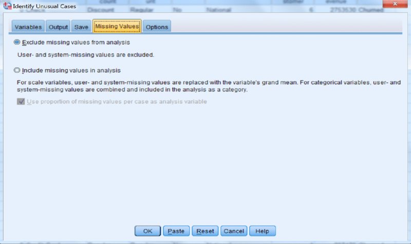
Figure 12.5 Identify Unusual Cases: Missing Values dialog
- Click the Options tab.
The Identify Unusual Cases: Options dialog (shown in Figure 12.6) allows you to specify the criteria for identifying unusual cases and to determine how many peer groups (clusters) will be created.
- The Criteria for Identifying Unusual Cases option determines how many cases are included in the anomaly list. This can be specified as a Percentage of cases with highest anomaly index values or as a Fixed number of cases with highest anomaly index values.
- The Identify only cases whose anomaly index value meets or exceeds a minimum value option identifies a case as anomalous if its anomaly index value is larger than or equal to the specified cutoff point. This option is used together with the Percentage of cases and Fixed number of cases options.
-
The Number of Peer Groups option searches for the best number of peer groups between the specified minimum and maximum values.
-
The Maximum Number of Reasons option controls the number of sets of reasoning variables in the Save tab. A set of reasoning variables consists of the variable impact measure, the variable name for this reason, the value of the case on the variable, and the value of the corresponding peer group.
We will just go with the default options as shown in Figure 12.6.
- Click OK.

Figure 12.6 Identify Unusual Cases: Options dialog
Identify Unusual Cases Output
The Case Processing Summary table (Figure 12.7) displays the counts and percentages for each peer group (cluster). In our data three clusters were found and the largest cluster was Peer ID 1 with a total of 1,659 cases or almost 50% of the sample.

Figure 12.7 Case Processing Summary table
The Anomaly Case Index List table (Figure 12.8) displays cases that are identified as unusual and displays their corresponding anomaly index values. This table lets us know who the unusual cases are, so now we can further investigate. In our data cases 714 and 1835 had the largest anomaly index values (3.925). This means that these cases had a deviation that is almost four times the average.
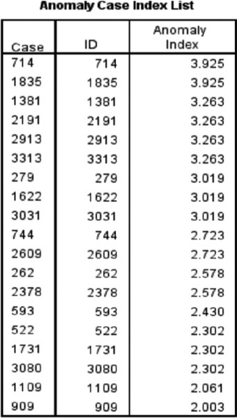
Figure 12.8 Anomaly Case Index List table
The Anomaly Case Peer ID List table (Figure 12.9) displays unusual cases and information concerning their corresponding peer groups. For example, we can see that Case ID 714 is in Peer ID group 1 and that this peer group has 1659 cases, which account for about 50% of the data file.
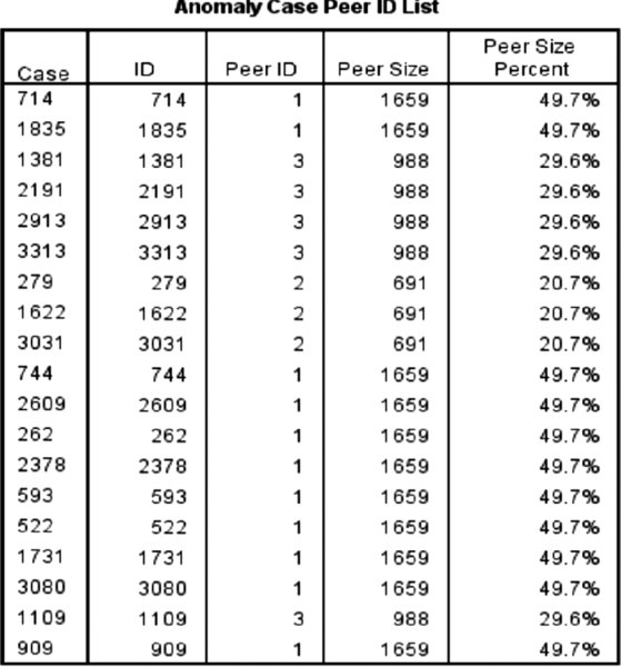
Figure 12.9 Anomaly Case Peer ID List table
The Anomaly Case Reason List table (Figure 12.10) displays the case number, the reason variable, the variable impact value (percentage of anomaly score due to that variable), the value of the case on the variable, and the norm (typical value) of the variable for each reason. As an example, Case ID 714 as we have seen has a high anomaly index score, 3.925 (see Figure 12.8). This case was most unusual on the variable Speakers. The contribution of this variable to Case ID 714’s anomaly index score was .678. Case ID 714 had a score of 411 on the Speakers variable while the mean score for peer group 1 on this variable was only 54.64. Note that if the variable impact value is low, it suggests that the case was classified as an outlier because of unusual values on more than one variable.

Figure 12.10 Anomaly Case Reason List table
So now not only do we know which cases are unusual, we also now know on what variables these cases are most unusual.
The Scale Variable peer group Norms table (Figure 12.11) displays the mean and standard deviation of each continuous variable for each peer group. The mean of a continuous variable is used as the norm value to compare to individual values.
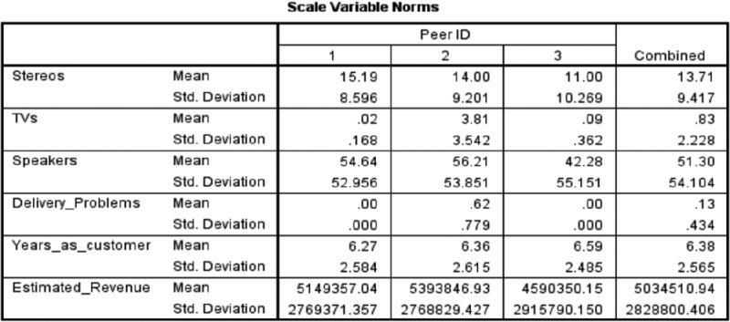
Figure 12.11 Scale Variable Norms table
The Categorical Variable Norms table (Figure 12.12) displays the mode, frequency, and frequency percentage of each categorical variable for each peer group. The mode of a categorical variable is used as the norm value to compare to individual values.

Figure 12.12 Categorical Variable Norms table
The Anomaly Index Summary table (Figure 12.13) displays an overall summary of the descriptive statistics for the anomaly index of the cases that were identified as the most unusual. You can see that for our data, 19 cases were identified as unusual and you can see the minimum, maximum, and mean values.
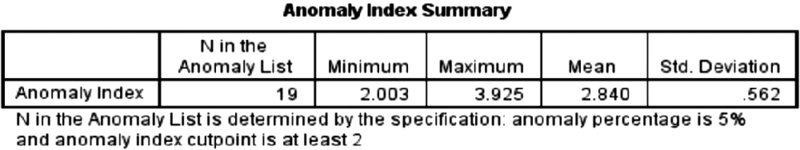
Figure 12.13 Anomaly Index Summary table
The Reason Occurrence by Analysis Variable table (Figure 12.14) displays the frequency and percentage of each variable’s occurrence as a reason. The table also reports the overall descriptive statistics of the impact of each variable. As was mentioned previously, only one variable appeared as the main reason for all of these outliers, and you can see the minimum, maximum, and mean values.

Figure 12.14 Reason 1 table
Now let’s take a look at the Identify Unusual Cases procedure created in the data editor.
- Switch to the Data Editor.
-
Right-click the AnomalyIndex variable and choose Sort Descending, as shown in Figure 12.15.
Figure 12.16 shows the new variables that were saved to the data file. As you can see, the data has now been sorted on the anomaly index value so it is easy to identify the unusual cases and begin further investigations. Now the researcher will need to determine if the unusual cases should be kept, removed, or modified.

Figure 12.15 Sorting data

Figure 12.16 New variables sorted
Optimal Binning
After exploring a data file, you often need to modify some variables. One common type of modification is to transform a continuous variable into a categorical variable; this is often referred to as binning. Note that since binning necessarily results in a loss of information, it should only be done where necessary. You might do this for several reasons:
- Some algorithms may perform better if a predictor has fewer categories.
- Some algorithms handle a continuous field by grouping it; however, you may wish to control the grouping beforehand.
- The effect of outliers can be reduced by binning.
- Binning solves problems of the shape of a distribution because the continuous variables are turned into an ordered set. Note that binning followed by treating a variable as a factor allows for nonlinear effects of predictors in a regression context.
- Binning can allow for data privacy by reporting such things as salaries or bonuses in ranges rather than the actual values.
SPSS Statistics has several procedures that allow users to bin continuous variables. For example, you can use the Visual Binning technique to create fixed-width bins (a new variable with groups of equal width, or ranges, such as age in groups of 20–29, 30–39, and so on). You can also use Visual Binning to divide a field into groups based on percentiles so that you create groups of equal numbers of cases. You can also use Visual Binning to create a field based on a z-score, with the groups defined as the number of standard deviations below and above the mean. Lastly, you can use Visual Binning to create customized bins.
Optimal Binning Dialogs
Optimal binning is another technique that bins a continuous field. Here, however, the transformation is based on the help of a separate categorical field that is used to guide or “supervise” the binning process. The transformation is done so that there is maximum separation between groups in the binned field’s relationship with the supervising field. The supervising field should be at least moderately related to the field to be binned. Note that this technique is only for continuous variables; however, the STATS OPTBINEX extension command (Data ➪ Extended Optimal Binning) extends this technique to allow binning of categorical variables by using the CHAID algorithm from the TREES procedure.
-
To use Optimal Binning, select the Transform menu, and then choose Optimal Binning, as shown in Figure 12.17.
The Optimal Binning: Variables dialog allows you to specify the variables to use in the analysis. You will need to place your categorical supervisor variable in the Optimize Bins with Respect to box and you must place at least one continuous variable in the Variables to Bin box. By optimally binning a predictor variable with the outcome variable, we create the ideal cutpoints to best separate—predict—the outcome’s values. Because the supervising variable must be categorical, this procedure can only be used with categorical outcome variables. However, you can always use another categorical variable in your data to bin a continuous predictor variable.
- Place the variable Status in the Optimize Bins with Respect to box.
- Place Stereos, TVs, and Speakers in the Variables to Bin box, as shown in Figure 12.18.
- Click the Output tab.
The Optimal Binning: Output dialog (Figure 12.19) allows you to specify what output you would like to view.
- The Endpoints for bins option creates a table for each binned variable that displays the cutoff values for each bin.
- The Descriptive statistics for variables that are binned option produces a table that shows the minimum and maximum values for each original field, as well as the number of unique original values and the number of bins that were created for each new binned field.
-
The Model entropy for variables that are binned option produces the entropy scores for each binned field. The transformation is done so that there is maximum separation between groups in the binned field’s relationship with the supervising field. If there is only one value of the categorical variable in a bin of the continuous variable, then the entropy is a minimum (equal to 0). That is the ideal, but the entropy will always be greater than 0 in practice.
Choose all of these options, as shown in Figure 12.19, so that we can discuss these.
-
Click the Save tab.
The Optimal Binning: Save dialog, shown in Figure 12.20, allows you to save binned variables to the active dataset. You can also choose to replace existing variables whose names conflict with the variables to be saved.
- Select Create variables that contain binned data values.
-
Click the Missing Values tab.
The Optimal Binning: Missing Values dialog, shown in Figure 12.21, is used to control how to handle missing values. Listwise deletion only uses cases that have complete data across all the variables that will be used in the analysis (this ensures that you have a consistent case base across all of the newly created variables). Pairwise deletion, on the other hand, focuses on each binned variable separately; therefore, it uses as much data as possible. However, this results in not having a consistent case base across all of the newly created variables. As mentioned previously, in our dataset we have no missing data, so in our case either option will produce the same result.
- Click the Options tab.
The Optimal Binning: Options dialog (see Figure 12.22) allows you to specify the maximum number of possible bins to create, identify criteria for bin endpoints, and define how to handle bins with a small number of cases.
- In the Preprocessing option, the binning input variable is divided into n bins (where n is specified by you), and each bin contains the same number of records, or as near the same number as possible. This is used as the maximum potential number of bins, by default 1,000.
- Sometimes optimal binning creates bins with very few cases. The Sparsely Populated Bins option allows for the possibility of merging small-sized bins with neighboring bins.
-
The last couple of options, Bin Endpoints and First/Last Bin, focus on bin criteria preferences.
We will just go with the default options as shown in Figure 12.22.
- Click OK.

Figure 12.17 Transform menu
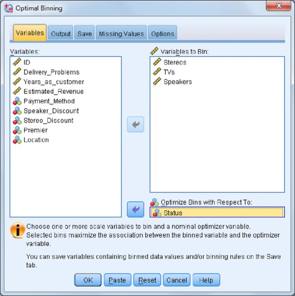
Figure 12.18 Optimal Binning: Variables dialog
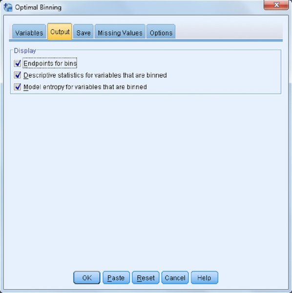
Figure 12.19 Optimal Binning: Output dialog
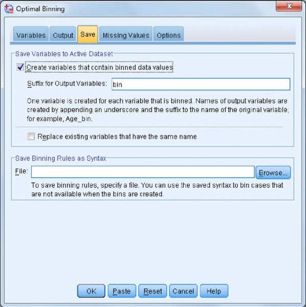
Figure 12.20 Optimal Binning: Save dialog

Figure 12.21 Optimal Binning: Missing Values dialog

Figure 12.22 Optimal Binning: Options dialog
Optimal Binning Output
The Descriptive Statistics table (Figure 12.23) displays the number of cases, and the minimum and maximum values for each original field, as well as the number of unique original values and the number of bins that were created for each new binned field. In our data we can see that two bins were created for the variables Stereos and Speakers, while three bins were created for the variable TVs.

Figure 12.23 Descriptive Statistics table
The Model Entropy table (Figure 12.24) shows the entropy values for each new binned variable. As mentioned in the table, lower entropy scores are associated with a stronger relationship between the binned and supervisor variables. In our case, all the entropy scores are similar; however, the new binned version of the variable, Stereos, has a slightly stronger relationship with the supervisor variable than the other binned variables.

Figure 12.24 Model Entropy table
The binning summary tables (Figure 12.25) display the number of bins for each newly created variable, as well as the endpoints. Furthermore, we can see how the newly created binned variables relate to the supervisor variable. In our data, for example, we can see that two bins were created for the variable Stereos and that the first bin captures all the values from negative infinity to one, while the second bin captures all the values from two to positive infinity (the presentation of these endpoints is controlled in the Optimal Binning Options dialog). We can also see that the first bin is associated with churned customers, since of the 422 cases in this bin, 361 (86%) are churned customers. Meanwhile, the second bin is associated with current customers, since of the 2916 cases in this bin, 1828 (63%) are current customers.
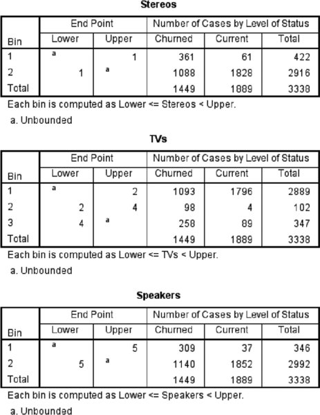
Figure 12.25 Binning summary table
We have now created binned versions of the variables: Stereos, TVs, and Speakers. As a simple test, we can do a quick analysis to determine if these binned versions of these variables are indeed more strongly related to the outcome variable, Status, than the original variables. To do this, we will run a stepwise logistic regression.
To use logistic regression:
- Select the Analyze menu, choose Regression, and then choose Binary Logistic.
- As shown in Figure 12.26:
- Place the variable Status in the Dependent box.
- Place the variables Stereos, TVs, Speakers, Stereos_bin, TVs_bin, and Speakers_bin in the Covariates box.
Choose Forward:LR in the Method box.
Now we have specified our outcome variable as well as the predictors. The Forward:LR method is a form of stepwise logistic regression that selects the predictor variable that has the strongest relationship with the outcome variable. It will choose the predictor variable that has the second strongest relationship with the outcome variable second (after controlling for any previously selected variables), and so forth. The Forward:LR method will stop once it can no longer incorporate additional significant predictors.
- Click OK.
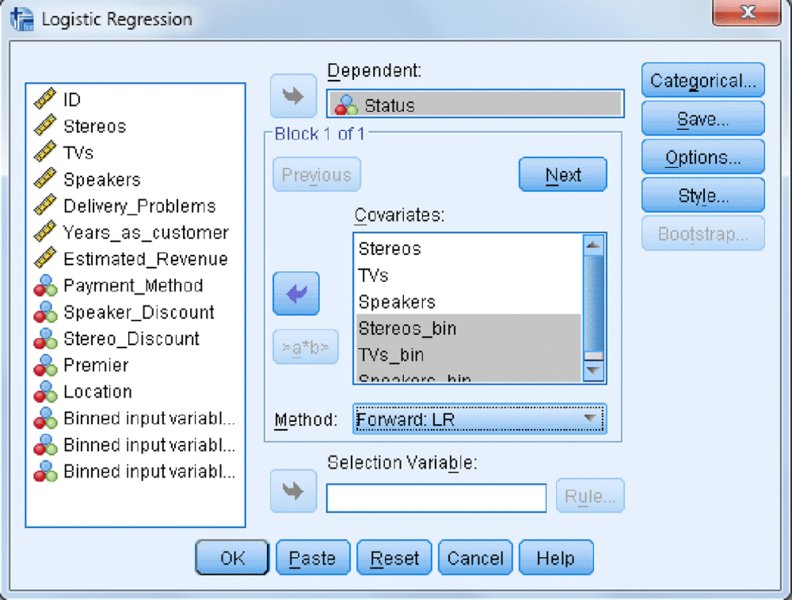
Figure 12.26 Logistic Regression dialog
Because the purpose of this logistic regression is just to show that the binned versions of the Speakers, TVs, and Stereos variables are more strongly related to the outcome variable, Status, than the original variables, scroll through the output until you find the output shown in Figure 12.27.
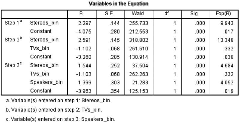
Figure 12.27 Variables in the Equation table
The Variables in the Equation table (Figure 12.27) shows that the first variable in the equation was Stereos_bin, and this is the variable with the strongest relationship to the outcome field status (incidentally, this is also the variable that had the lowest entropy score). The second variable admitted into the model was TVs_bin, and this is the variable with the second strongest relationship to the outcome variable after controlling for the previous variables in the equation. The third variable in the model was Speakers_bin, and this is the variable with the third strongest relationship to the outcome variable after controlling for the previous variables in the equation. Note that in this simple demonstration, all of the binned variables were chosen over their continuous counterparts; thus, the Optimal Binning procedure successfully created binned variables that maximized the relationship between the supervisor variable and the variables of interest.