Chapter 14
Powerful and Intuitive: IBM SPSS Decision Trees
Now that we’ve seen Artificial Neural Nets, we are going to move on to another technique. Decision trees are more accurately thought of as a class of techniques as they represent multiple algorithms. The chapter that lays the groundwork for what we will see in this chapter, and all of Part III, is Chapter 11. If you are new to data mining, in general, you may want to start there. IBM SPSS Decision Trees offers four “Growing Methods”: CHAID, Exhaustive CHAID, CRT, and QUEST. The C5.0 Tree extension command offers a fifth possible option. Extension commands will be discussed in Chapter 18. We will demonstrate just CHAID and CRT, but running more than one iteration of each. CHAID and CRT provide a number of contrasts to each other so those two will give a good understanding of the decision tree approach. By altering the settings of both CHAID and CRT, it will allow the differences to become even more clear. A deeper understanding of two will prove a more satisfying introduction than a brief introduction of all five. (Note that Exhaustive CHAID, as the name implies, is quite similar to CHAID.) Finally, at the close of the chapter we will demonstrate the Scoring Wizard.
Building a Tree with the CHAID Algorithm
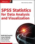
We’ll use the Titanic_Results.sav dataset (available in this chapter’s downloads), and the same partition variable, Train_Test, that was created near the end of Chapter 13. As shown in Figure 14.1, Pclass, Age, Sex, and Parch (as scale) will be chosen as Independent Variables. Train/Test validation using a partition variable is not the only method, however, and alternatives are covered in the “Alternative Validation Options” section near the end of this chapter.
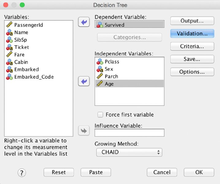
Figure 14.1 Decision tree main menu
Notice that the button for the Validation submenu is selected in Figure 14.1. We move to that submenu next. Note the symbols next to the variables in the figure indicating level of measurement. Different levels of measurement declarations in the Variable View could result in a different tree, as the algorithm will treat nominal, ordinal, and continuous independent variables differently.
Restricting the variables like this is temporary while you get used to this new technique. Once we review the basics, we will be using all of the available variables. Tree algorithms are generally quite good at performing feature selection as part of model building.
As mentioned, we will also perform a couple of iterations to show what it is like to repeat the model a number of times. In statistics, confidence in one’s result comes from carefully choosing a single approach that is recommended by theory. When using these predictive modeling techniques rigor comes from systematically attempting all plausible options, carefully documenting what you have tried, and validating all attempts against a hold-out sample (or similar alternative approaches like N-fold validation). The choice of the final model is justified empirically, not on theoretical grounds.
The partition variable is declared in the Validation submenu shown in Figure 14.2. Using an external variable is not the default, but the necessary choice is easily indicated. Select “Use variable” and indicate that we will “Split Sample By” Train_Test.
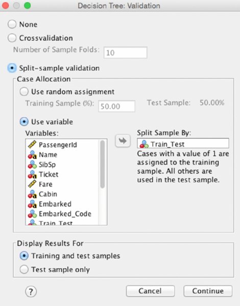
Figure 14.2 Validation submenu
Otherwise, we will let the model run on defaults. The result in the output window shows us the Training Sample tree, shown in Figure 14.3, as well as the Test Sample tree, shown in Figure 14.4. The shape of the two trees will be the same since the shape was built using the Training Sample only. However, the tree can be thought of as a set of rules. For instance, this rule:
- If Female and First/Second class then Survive
can be applied to any other data. So the Test Sample tree has the identical shape to correspond to the same rules, but the values are drawn from the Test dataset so the exact values will be somewhat different. However, since the Train and Test datasets were chosen at random, they are structurally the same—they have the same variables and the same possible categories. Any future dataset for which you used the tree model to make predictions would also have the same variables and categories.

Figure 14.3 Training Sample tree

Figure 14.4 Test Sample tree
For example, let’s consider the rule involving female passengers in First or Second class, the survival rate in the Training Sample is 95.5%, but a tad lower at 93.2% in the Test Sample. (The relevant information is in Node 3 in both cases.)
While we are at it, let’s review some more details of the tree using the Training Sample. Remember that the Training Sample tree is the one shown in Figure 14.3. We observe the following:
- The “Root Node” (Node 0) reveals that we have a total sample size of 608, of which 38.7% survived.
- The most important variables are Gender and Pclass, in that order.
- There are four “leaf nodes” (Nodes 3, 4, 5, and 6). Their sample sizes add up to 608, and they represent a mutually exclusive and exhaustive segmentation of the sample.
- The lowest survival rate is found in Node 6 (15.9%) and the highest (95.5%) in Node 3.
Finally, if we observe the survival rates for the same nodes, 6 and 3, but this time in the Test Sample tree, Figure 14.4, we find that while they are not identical, they show a similar pattern.
Next we will consider our overall accuracy. Figure 14.5 gives us a report of the performance of the tree as a whole. There are four figures in the table that we will focus on:
- The Training Risk Estimate: .220
- The Test Risk Estimate: .198
- The Overall Percentage Correct for the Training Sample: 78.0%
- The Overall Percentage Correct for the Test Sample: 80.2%

Figure 14.5 Overall accuracy results
The “Risk” is simply a measure of inaccuracy. Why report for the training sample .22 wrong instead of .78 correct? This is because, by reporting that along with a standard error, you can build a confidence interval around it. When reporting to others, the more salient facts will be the stability in the form of comparing the training accuracy to test accuracy (here 78.0% and 80.2%), and the test accuracy. The accuracy for the test sample is especially important since it is based on “unseen” data, but the most conservative approach is reporting the lower accuracy of the two. This result would be considered stable, but a closer level of accuracy between the two would have been desirable. In other words, the test accuracy is OK, but it would be nice to do better. However, the fact that the test accuracy is even better than the training accuracy certainly makes the model appear stable. If the test accuracy were much worse than the training accuracy we would be concerned about stability.
It is noteworthy that the tree didn’t grow all that much. We only have four leaf nodes. We will make some changes to our settings and give this another shot. First, however, let’s review what CHAID is doing behind the scenes to produce the tree.
Review of the CHAID Algorithm
Note that Sex was the first split variable. It was chosen over Pclass. Let’s refer to the Crosstab results, which have been produced using the Crosstab menus, shown in Figures 14.6 and 14.7, to explore why. Although both Sex and Pclass have Asymptotic Significance results (p values) that are very small, and well below .05, the result for Sex is smaller. That is why Sex is the top branch of the tree.

Figure 14.6 Crosstab results for Sex variable
Figure 14.7 Crosstab results for Pclass variable
We’ve just seen that in CHAID the top branch is awarded to the lowest p value, but in actuality, our Crosstab demonstration is concealing a step. First, we have to determine if our ordinal variable will collapse any categories. Reference to the tree diagrams will show that collapsing has, indeed, occurred. However, the left branch and right branch differ. Why is this occurring? To answer, we need a more descriptive Crosstab result. As shown in Figure 14.8, we need to split on gender to show that the Pclass crosstab, when examining only females, is different when we examine only males. We noticed that the survival rate for First class and Second class females is actually very similar—96.8% and 92.1%—so the CHAID algorithm first collapses them and uses the two-category version of Pclass for a new Chi-Sq p value (not shown). For males, Second class and Third class are very similar (15.7% and 13.5%) so the CHAID algorithm collapses those two categories. Scale variables pose an interesting problem because Chi-Sq is not designed to investigate scale variables. CHAID buckets scale variables into deciles (a default setting which can be changed), and then treats them as ordinal variables. While the results work pretty well, recognize that the boundaries between the deciles are essentially arbitrary. These differences in treatment serve as an important reminder that the independent variables must have their levels of measurement declared properly in the very first step (Figure 14.1). We will see later that CRT finds boundaries with a more granular level of precision using a very different approach.

Figure 14.8 Crosstab showing all three variables
Adjusting the CHAID Settings
In order to let the tree grow more aggressively, we will allow for a depth of 5 and smaller Parent/Child sizes, as shown in Figure 14.9. One could also describe the result as being more flexible, or even more “liberal” as the word is used in statistics. In short, the tree will become a larger tree with more branches and leaf nodes, as shown in Figure 14.10. We will also allow all of the available independent variables to be used (not shown). There is nothing magic about these adjustments. Given our sample size the default settings of 100 and 50 are a bit high. Is a maximum tree depth of 5 too aggressive? It is more aggressive than 3, but we are simply responding to the fact that we got a fairly parsimonious tree on the first attempt, so we are attempting to get a more “bush like” tree with more branches. If the more aggressive settings produce an unstable tree, we have a failed experiment. If it is more accurate (bush-like trees are always more accurate on the training sample), but also stable (accurate on both training and test samples), then we have a successful experiment.

Figure 14.9 Decision tree criteria

Figure 14.10 Training tree after changing settings
The tree is much expanded. The top half of the tree (Train Sample) is the same. Three new variables have joined Sex and Pclass: Embarked Code, Age, and Fare. Embarked Code represents where the passenger boarded the Titanic. It made three stops in Europe before entering the North Atlantic. The new variables create a more granular tree, and we now have a segment with a lower survival rate than we saw in our Training Sample tree before. Node 12 has a survival rate of 9.5%. Note that Age has been split (or rather its deciles have been collapsed down to two categories). Those missing Age have a survival rate somewhat like the passengers over 14 years of age so CHAID has combined them with this group. We will see that CRT has a very different approach. Fare has also been collapsed down to two groups even though it too would have started with deciles.
Let’s examine the accuracy and stability of this example using the results shown in Figure 14.11. It won’t always be the case, but we achieved considerably better results on the second try. Sometimes you might need a compromise between the conservative and aggressive settings. You may also choose to change the settings shown in the CHAID tab (not shown). These settings would include changing from 95% confidence levels to something either more or less aggressive like 90% or 99%. Lowering to 90% would allow for an even larger tree. Raising to 99% would make it more conservative, resulting in a potentially smaller tree. A half dozen or even a dozen different versions of settings for just the CHAID algorithm would not be unusual. Because it is more accurate, and quite stable (even better performance on the Test is always nice) this model is now in first place, and we will try another algorithm. It is worth noting that it is more common to have a slight degrading of performance on the test. Having better performance on the test is less common. However, the more important fact is that the numbers are fairly similar, indicating stability.

Figure 14.11 Accuracy results for the larger tree
CRT for Classification
Set the configuration for this example in the dialog shown in Figure 14.12. We will change the Growing Method to CRT, but not make any other changes. All of the possible inputs will be used (which was the case for our second CHAID attempt). The variables as shown are Pclass, Sex, Parch, Age, SibSp, Fare, and Embarked_Code. As we noted with CHAID, remember that the Level of Measurement declaration has an impact on the outcome. Validation remains the same—use the Train_Test variable. For Criteria use the settings we just chose for the second CHAID attempt—depth of 5, 30 for parent minimum, and 15 for child minimum. The result, shown in Figure 14.13 is a much larger tree.
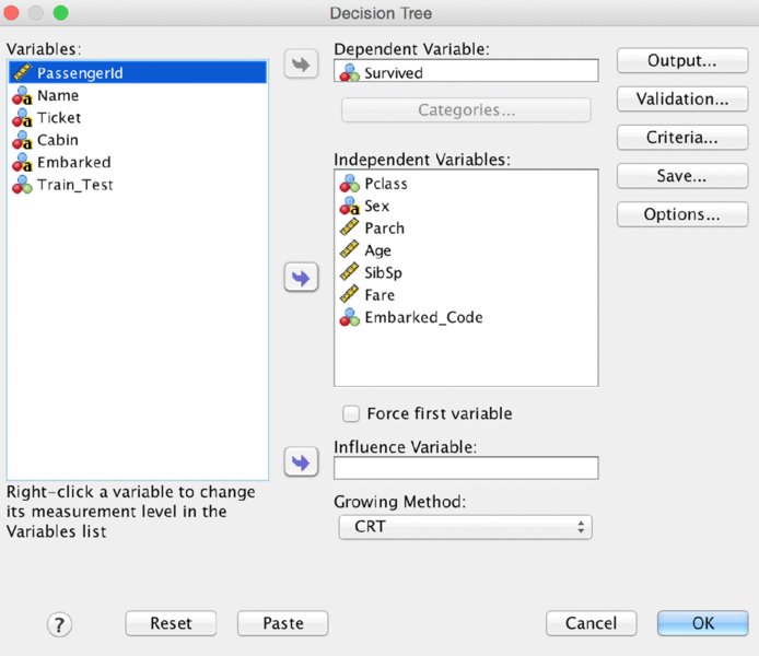
Figure 14.12 Decision tree main menu

Figure 14.13 Intial CRT tree
CRT has produced a considerably more complex tree. Its performance is about the same as the second CHAID attempt. It is also fairly stable (see Figure 14.14). Note that it uses Age as the second most important variable for males. Also, Fare is used multiple times with subtle and tiny little differences between the cut-off points.
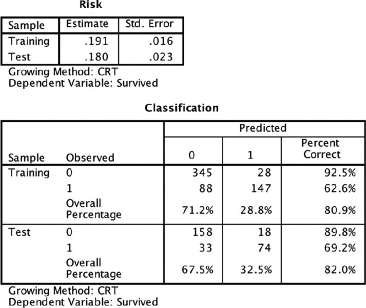
Figure 14.14 Accuracy results for CRT tree
Understanding Why the CRT Algorithm Produces a Different Tree
The CRT algorithm was first described in 1984 by Leo Breiman, Jerome Friedman, Charles J. Stone, and R.A. Olshen in their book Classification and Regression Trees (Chapman and Hall/CRC). However, a key component of the approach is to use the Gini Coefficient, which is 75 years older. Sociologist Corrado Gini’s Gini Coefficient is used to describe income disparity in countries. A Gini Coefficient of zero would describe a country where everyone has the same income, and a Gini coefficient of 1 means that one person has all the income. The CRT algorithm repurposes this in a clever way. Ultimately the goal of a decision tree is to identify leaf nodes where there is no “disparity” in the target variable. Alternate vocabulary serves us better in the context of a decision tree. In a “pure” leaf node, all values of the target variable would be the same. So, when using CRT or adjusting settings we generally use the words “purity” and “impurity.”
So there are two key observations to make about the fact that CRT selected Sex as the first variable. First, CRT always produces a binary split. CHAID, as we have seen, does not always do so. So two trees, one CHAID and one CRT, will tend to look quite different, but may be similar, or even identical in their predictions. Second, since reduction in impurity is a goal, Sex must have produced a substantive reduction in impurity. The overall survival rate is about 40%, which is not terribly far away from the percentage that would maximize impurity. A binary target with 50% in each category would achieve that. In contrast, after splitting on Sex, the survival rate for females climbs, moving away from 50% within Node 1, and the opposite occurs for Males. CHAID’s search for the lowest p value tends to produce the same effect, but with CRT we move rather directly to the goal of pure leaf nodes. If you reflect carefully on this approach, you should grow concerned. A leaf node with only one case will always be pure. This is disconcerting, but the CRT algorithm addresses this by weighing “balance” equally with the reduction in impurity. While Nodes 1 and 2 are not equal in size, their sizes of 212 and 396 are not terribly out of balance. The Sex variable was the strongest option when weighing both purity and balance, and therefore CRT split on Sex first.
Scale variables are handled elegantly in CRT. It need not transform them as an initial step. As we have seen, CHAID converts scale variables into deciles and then treats them as ordinal variables in later steps. CRT’s algorithm considers every possible cut point. Naturally, the first and last cut points would produce a very unbalanced split, but it calculates them all. In the instance of this dataset we see that young boys have a much higher survival rate than male teens and adults. Of all the possible cut points for age, 13 years old was the optimal for purity and balance. And of all the possible variables with which to subdivide Males, Age was the best.
Missing Data
Surrogates are a fascinating solution to the problem of missing data. In contrast to CHAID, CRT does not treat missing data as a separate category. A substantial number of passengers are missing a value for age in the Titanic data, for instance. CHAID’s behavior in this regard makes its treatment of missing data rather transparent because you can easily see where the cases with a missing value are in the tree. Instead, when CRT encounters a missing value, it attempts to determine whether that case should join the left branch or the right branch. What is brilliant about the solution of using surrogates is that it does not require a very precise estimate of age. Imputation, a well-known technique, would involve trying to estimate the passenger’s age, producing an estimate such as 5 years old, or 48 years old. With surrogates, we simply need to identify if the passenger is more likely to be younger or older than 13 since that was the threshold that we just discussed. CRT identifies five variables from among the variables specified for the tree that allow us to make this determination. If they are traveling with a spouse or their own children, for instance, they are certainly unlikely to be under 13 years old. Each node has up to five surrogates, and obviously they will be different depending on what is missing. The five variables will be those five that the complete data reveals to be the most correlated with the missing information.
Changing the CRT Settings
We can change a number of settings with CRT to produce a larger or smaller tree. We could change the maximum depth or the parent/child settings. We could also change the “minimum change in impurity” found on the CRT tab, which has a line of coaching on the effect of increasing or decreasing this setting: “Large values tend to produce larger trees.” Try adding or dropping a zero (or two) at first so that you have more or fewer decimal places. That should serve as a guideline for how much of a change will have a noticeable effect. We will only be attempting one additional CRT tree in this chapter, and will choose Pruning as the criterion to change. This is a terribly important setting, is how CRT is designed to work, and frankly should be on by default. It can be interesting to examine an unpruned tree as an exploratory step, but generally this setting should be turned on. The Pruning submenu is shown in Figure 14.15.
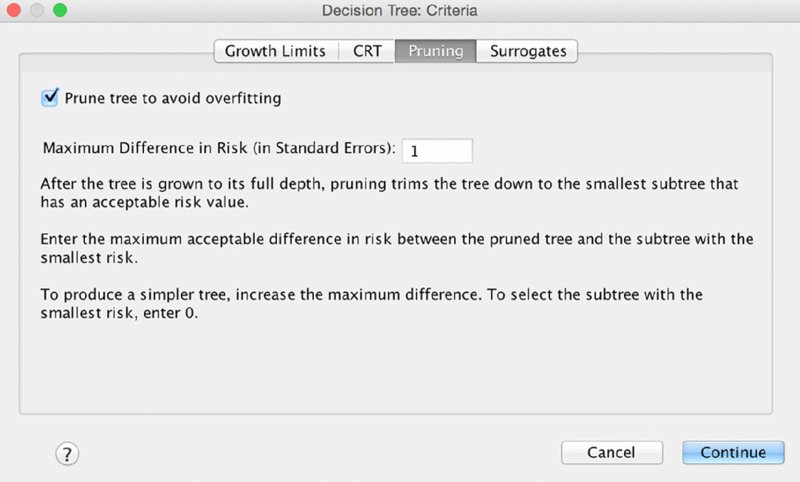
Figure 14.15 Pruning criteria submenu
The resulting tree is very different, and much smaller (the Training Sample tree is shown in Figure 14.16).

Figure 14.16 Second CRT tree
The original developers of the CRT algorithm approach (Breiman et al.) experimented with a number of variations on the algorithm and discovered that the best results were found when they grew a tree aggressively and pruned it back. This was better, for instance, than constraining the growth of the tree without pruning. What “cost complexity” pruning attempts to do is remove those branches that have more complexity than they are “worth.” Branches that increase accuracy enough are worth it, but branches that fail to increase accuracy enough are not. It is this ratio between complexity and the increase in accuracy that is being weighed.
The stability is quite good—the Overall Percentage accuracy is similar in both the Training and Test samples. The accuracy is also good, at 83.4% for the Test data. It actually appears to be the best so far, as shown in Figure 14.17.

Figure 14.17 Second CRT tree accuracy results
Comparing the Results of All Four Models
Let’s compare the results of the four models. We can apply many criteria in comparing and contrasting these results. Table 14.1 shows just one possible way to examine the results in a table. In data mining consulting work, it is not unusual to consider more than 100 models using many algorithms and dozens of settings.
Table 14.1 Comparing our four tree attempts
| First CHAID | Second CHAID | First CRT | Second CRT | |
| Number of Variables Used in Tree | Two | Five | Five | Three |
| Number of Leaf Nodes | Four | Seven | Ten | Four |
| Highest Survival Rate (Train) | 95.5% | 98.6% | 95.5% | |
| Lowest Survival Rate (Train) | 15.9% | 0% | 5.9% | |
| Settings | Default | Increased depth, and reduced Parent/Child | Reduced Parent/Child | Reduced Parent/Child and Pruning |
| Train Accuracy | 78.0% | 80.6% | 80.9% | 79.6% |
| Test Accuracy | 80.2% | 82.3% | 82.0% | 83.4% |
Given the results here, we would probably be inclined to go with the Second CRT. We’ve been lucky in that all four are stable. None have a dramatic gap drop in accuracy moving from Train to Test. In fact, all did better in the Test, so all are viable in that sense. The last one has somewhat better Test accuracy, and once we establish stability we don’t care that much about Train accuracy. Finally, the fourth model is even somewhat parsimonious. It is not an overly complex tree. With that in mind, we will save the predicted values as a new variable in the dataset to be used in the next chapter. We will close the chapter with a discussion of the Scoring Wizard, using our best model for the example. But first, we will discuss alternative validation options.
Alternative Validation Options
Let’s consider an alternative setting for our validation. We have been using the same variable, Train_Test, in order to compare multiple algorithms. It is possible, and quite easy, to have SPSS generate partition variables as shown in Figure 14.18. Note that we’ve chosen 70% for the Training Sample because the sample size is a bit small in the Titanic dataset. When faced with that challenge it is usually recommended to increase the Training Sample somewhat, just as we did with the Train_Test variable.

Figure 14.18 Using a random assignment
The results when rerunning with the same settings as the second CRT tree indicate a lower value for Test accuracy, 80.8%, than for Training accuracy, 81.1%. The steps in creating the tree are not reshown, but the Risk results are in Figure 14.19.

Figure 14.19 Results using the random assignment
This pattern, of higher Train accuracy, is more typical than higher Test accuracy. As we have seen several times in this chapter, it is not impossible to have higher Test accuracy, but the pattern in Figure 14.19 is more common.
You may have noticed another option in Figure 14.18. Although we will not repeat our analysis using this option, cross-validation works in the following way. Crossvalidation divides the sample into a number of subsamples, or “folds.” The default is 10, but you can specify up to 25 sample folds. Each time a different fold is withheld. For example, if you choose the default of 10, the first tree would use 90% of the data to build the tree, and 10% (the first 10%) as the test data. Crossvalidation reveals a single, final tree model in the output. The risk in the output is the average risk of all the trees.
The Scoring Wizard
In order to show the Scoring Wizard, we are going to save our model as an XML file as shown in Figure 14.20. While we are going to demonstrate only one scoring method, there are actually numerous options. For example, the TREES procedure (the SPSS Syntax command for producing decision trees) offers a number of other formats for saving the rules that may be useful in other scoring contexts. The RULES subcommand of the TREE procedure allows you to generate SQL statements. If you are new to SPSS Syntax, you will want to read the chapters in Part IV of this book, starting with the introduction to SPSS Syntax in Chapter 16. It is not uncommon to find features—like the SQL rules option—that are available in SPSS Syntax, but are not found in the menus.

Figure 14.20 Scoring Wizard first menu
To be consistent with the figures, be certain to use the settings of the second CRT model that we’ve decided was our best option.
Now load a different data file. We will use the Titanic_Test.sav file. This file contains the same variables except that it is lacking the Survived variable. A willing suspension of disbelief is required here. We all know that the Titanic sank a hundred years ago, so naturally we know the outcome of all of the passengers, but we are going to pretend to not know the outcome for the Test data. We are going to use our Train dataset’s model, but use it to score the Test dataset. This is a bit different in SPSS Modeler, as we have seen with its unique partition node, and so on, but SPSS Statistics is quite capable of doing a hold-out sample validation as well, and it does it quite elegantly as we are about to rehearse. Please ensure that Titanic_Test.sav is not only open, but is the active file.
The Scoring Wizard is found in the Utilities menu. It will list any .xml files that can be used. Note that it may also display .zip files that you might have on your machine. We are only interested in the file that we just made: TitanicModel .xml. The opening screen is shown in Figure 14.21.

Figure 14.21 Scoring Wizard second menu
SPSS wants to verify that the variables referred to in the model are also found in the Test dataset, shown in Figure 14.22. They should indeed align, which allows us to continue.
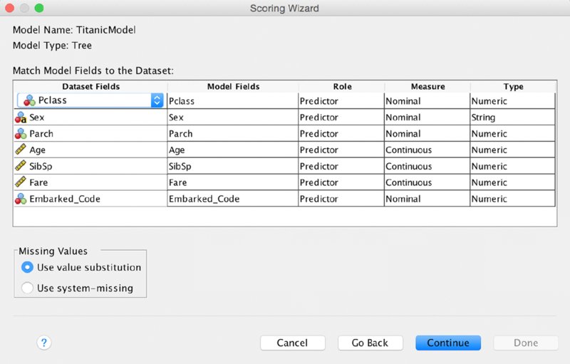
Figure 14.22 Scoring Wizard third menu
Finally, we have to decide which new scored variables are to be created by the Scoring Wizard. These differ by model type, and are affected by what we requested when we built the .xml file. We will request the latter three choices: Node Number, Predicted Value, and Confidence as shown in Figure 14.23.

Figure 14.23 Scoring Wizard fourth menu
The predictions for the Test passengers should now be visible in the data window, Figure 14.24. (The Name variable has been moved to make it easy to view the predictions.)

Figure 14.24 Predictive scores for some passengers in the Test dataset
We covered the Scoring Wizard in some detail, showing each screen, but as you can see it is really quite straightforward. It is one of many SPSS Statistics features that fewer people know about than those that can benefit from it. For instance, many SPSS Statistics users use linear regression, but few also know that they can score new records with their regression model using this same menu.