Chapter 16
Write More Efficient and Elegant Code with SPSS Syntax Techniques
Many SPSS users rarely (or never) use SPSS Syntax. Others remember when Syntax was the only way to interact with SPSS. Back in the ’90s, not everyone embraced the graphical user interface (GUI) at the same time or to the same extent. The GUI definitely leapt forward around the time of Windows 95. It is easy to forget that SPSS was already in its fourth decade at that time, first written in 1968! Now, few SPSS users ignore the GUI completely. However, the reverse, predictably, has occurred—many SPSS users don’t learn about Syntax. If you are among them, why learn now? If you are rusty, what is the latest news regarding Syntax? If you are expert, are there any commands that you might be missing out on?
When I (Keith) was first faced with SPSS in college (late ’80s), my project advisor dropped a very big and very heavy tome on the desk. It was the programming manual for SPSS-X, an older version of SPSS that would have forced me to learn SPSS Syntax in earnest. I was studying computer science so I wasn’t particularly reluctant about using code, but having to worry about statistics theory, the specifics of the project, deadlines, and learning a new programming grammar all at the same time was daunting. Fortunately, I had just won a research grant. It was a small grant, but it allowed me to purchase my own copy of the much newer version of SPSS with a graphical user interface. It reduced the amount left over to pay me for the research considerably. My advisor thought that quite a prodigal move given my age and resources, but I somehow knew that it would pay off in the long run. My coauthor, Jesus, had a similar initial frustration with Syntax, which he describes in the next chapter.
Why did I avoid Syntax at the time, and why do I embrace it to such an extent now? Frankly, Syntax has a bit of a learning curve, which I feared would slow me down. I was more enthusiastic about the results, and wanted to jump right in. Also, I was at the stage in the project during which I was exploring data. I’ve always felt that the menus make that easier and faster. However, when the analysis becomes routinized and repetitive, switching to Syntax can increase efficiency by an order of magnitude. I can say without exaggeration that some analyses are simply not possible (or at least not practical) without some coding. Quite simply, you can’t be a power user of SPSS without it.
The goals of this chapter are to move you along to your next milestone in your journey of using Syntax, and to prepare you for some of the topics in this section of the book. Many SPSS users are a bit intimidated by Python and R, for instance. One can actually make the argument that as a programming language Python is easier to learn than Syntax. However, you have to get used to using code, and not clicks, to control SPSS. What if you are already using Syntax? Your next milestone is learning about commands that cannot be pasted from the menus, which means learning of their existence, adopting strategies that use them, and writing better and more readable code as a result. Even if you are doing all of that, this chapter reviews those topics in a way that prepares you for the chapter on programmability and extension commands, Chapter 18.
The themes of this chapter are efficiency, elegance, and readability/maintainability. Efficiency is simply working smart, and ultimately working briskly. Computers are generally pretty quick, so efficiency means working on the slower half of the human/computer interface. It means getting past performing tasks like pointing and clicking the same steps repeatedly, or needless copying and pasting. Elegance is about writing code that is easy to read (by our colleagues and ourselves), correct, and easy to maintain. Code that is easy to read and easy to maintain is relatively short and easier to validate. Code that is hundreds of pages long is a challenge on both counts. Easy to read implies well-documented code. Easy to maintain involves concepts like parameters and loops, which we will explore. These techniques allow us to keep our code reasonable in length.
We are going to take precautions and assume that you haven’t used Syntax at all before. We show how to “paste” commands and review the grammar. This is a brief transition before the real nuts and bolts of the chapter: using Syntax well and being brilliant in the basics of Syntax.
A Syntax Primer for the Uninitiated
If you’ve never used Syntax before, the best place to start your journey is not with typing in a blank syntax window, but rather with using the Paste button. This is not the same as “cut and paste,” as we will see. Consider the Frequencies dialog shown in Figure 16.1. The Paste button is shown at the bottom of the dialog on the left. (Its position on a windows version will be somewhat different.)
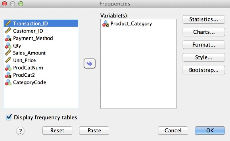
Figure 16.1 Frequencies main dialog
Let’s examine the results as they appear in the Syntax window, shown in Figure 16.2.
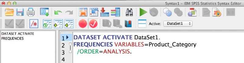
Figure 16.2 Resulting Syntax in the Syntax Editor
Note that the SPSS Syntax window is not merely a text editor. It has features specifically designed to help you write Syntax. On the left is a list of commands. At the moment, we have just two. On the right we have line numbers and the complete Syntax code. The color coding is important; you can see it when working in the Syntax window. Commands are blue, and appear right up against the left margin. Back in the day, when punch cards were still used, starting commands in the first column was a requirement but that is no longer the case. The use of capitals is not required, but it is conventional to use uppercase for commands. In contrast, variable names, like Product_Category, are conventionally typed in mixed case or lowercase.
Our first command is DATASET ACTIVATE. This can be valuable when using multiple data windows, but we will set aside our discussion of this command until later. The second command, FREQUENCIES, is the command we were expecting because it is the dialog that we are working in. Subcommands appear in green. We have one subcommand, /ORDER. The subcommands allow you to take advantage of the potentially numerous features of the commands. In the Syntax Reference Guide, available in the Help menu, you will find many pages dedicated to some of the more complex commands. They can have numerous subcommands. Some keywords are also reserved words—words are not available to be used as variable names. While it is sometimes possible, it is rarely a good idea to use any variable name that could be confused with commands or keywords. When Syntax users speak of keywords they generally mean the words appearing in a maroon color in the editor. In this case, the ANALYSIS portion of /ORDER = ANALYSIS is this part of the command. The ORDER subcommand indicates that we want to designate the order, and ANALYSIS makes explicit what order we would like. Variable names, filenames, and so on appear in black. They do not belong to the language, but are rather referring to the specifics of our dataset.
Note well that both commands—not all three lines—end in periods. This is critical. If we violate this rule, the color coding will change, and we run a considerable risk of an unexpected result or no result at all. Note as well that the subcommand is indented and has a slash. The indentation is not as critical as it was in the punch card days. The slash punctuation, however, remains very important.
Two important buttons are visible in Figure 16.2. The Run Selection button, which looks like a “play” button, is indicated with a green arrow and can be used to run selected code. Four icons to its right is the symbol showing a page and question mark. It is the Syntax Help button. An example of Syntax Help is shown in Figure 16.3.
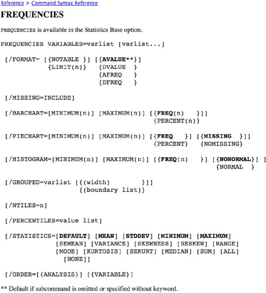
Figure 16.3 Syntax Help
The results of requesting Syntax Help might be a bit different than you were expecting. It is essentially a grammar chart. There is hypertext in the document that takes you to examples and explanations of the command, but the primary purpose of this button is to show you the available subcommands, and available choices for each subcommand. Notice, for instance, that in lieu of /ORDER = ANALYSIS we could have chosen /ORDER = VARIABLE. Brackets ([ ]) indicate that the entire subcommand or a portion of it is optional, and braces ({ }) indicate our choices on the subcommand.
Note that virtually everything is optional. We could actually type the following, and it would run just fine:
FREQ Product_Category.
In contrast, the full command, as SPSS pastes it into the Syntax Window, appears in Figure 16.4. Note that the code has been highlighted which is required is you are going to use the Run Selection button (green arrow icon) which we discussed earlier. The menus also offer you the option to Run All (not shown) which would not require this step.

Figure 16.4 Frequencies command in the Syntax editor
You won’t want to get bogged down in the details. The key point is that pasting easily produces accurate Syntax that we can save and rerun when we need the same result in the future. However, that doesn’t mean that you will never want to modify the result. In particular, pasting on default settings will produce an EXECUTE command. See the side bar on this subject.
This rapid-fire review is enough to get you through the chapter, but if it is a brand new topic to you, you should read the following chapters of the Command Syntax Reference:
- Introduction
- Universals
You can find this extensive (and huge) document in the Help menu, as shown in Figure 16.5. Note that the Help menu in version 24 is abbreviated and doesn’t have as many options listed, but the Command Syntax Reference is still available in the menu. Don’t get dissuaded by the size of the document—the two recommended chapters are manageable.
Figure 16.5 Help menu showing the Command Syntax Reference
Making the Connection: Menus and the Grammar of Syntax
Understanding commands, subcommands, and keywords is very easy if you compare some pasted Syntax to the dialogs. The name of the dialog corresponds, sometimes exactly, with the command. The subcommands are generally modified via subdialogs and the keywords are modified with check boxes. This is not always followed in the design of the dialogs, but using two commands as examples we will explore how the dialogs and the resulting Syntax relate to each other. We will take a closer look at the familiar Frequencies and Crosstab commands.
The first example of the command (Figure 16.6) was done with default settings (Lines 1–2). “Old school” syntax practitioners who mastered syntax without the menus sometimes find the “extra words” distracting, but it is harmlessly making the defaults explicit. Line 4 provides an example stripped of the defaults.
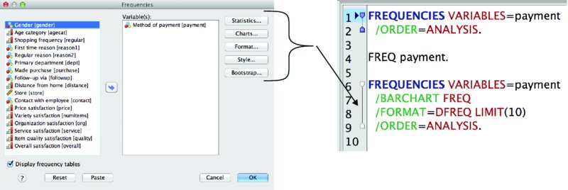
Figure 16.6 Frequencies dialog and Frequencies commands
Noteworthy is the near one-to-one correspondence between the rectangular buttons in the upper right-hand portion of the menus, and the three pasted commands (Lines 6–9). /BARCHART, inserted with the Chart button, and /FORMAT, inserted with the Format button, are two examples. The Charts subdialog, accessible by pressing the Charts button, is shown in Figure 16.7.
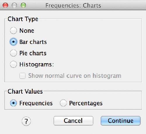
Figure 16.7 Charts subdialog
Figure 16.7 shows the check boxes within the menus. In this case, Bar Charts have been requested and that is visible in the syntax as the /BARCHART subcommand with the keyword FREQ. Figure 16.8 shows the Crosstabs main dialog and the Cell Display subdialog.
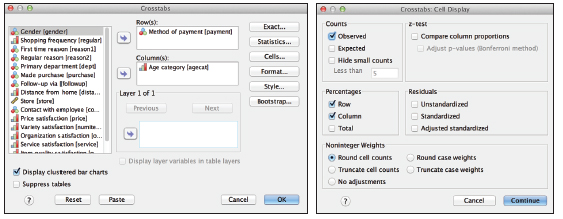
Figure 16.8 Main dialog and Cell Display subdialog
The CROSSTABS command provides an additional example of the relationship between the dialogs and the commands. The first pasted bit of code (Lines 11–15) imitates our last example in that it was pasted with default settings. Line 17 in Figure 16.9 shows an example that has been typed with abbreviations. Though this is an old style, it is not just nostalgia. Because you will find collections of code written like this lurking about in organizations that have been using SPSS Syntax for decades, seeing it might help you understand why it looks that way.
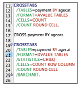
Figure 16.9 Three CROSSTABS examples
Let’s examine some of the specifics of this example. In the third example of the CROSSTABS command (Lines 19–25) you can see the keywords that have been chosen. The format has been changed—Line 21. The choice of the Chi-Square statistic (check box not shown) adds a new subcommand with keyword CHISQ. The additional, non-default check boxes Row and Column are visible on Line 23. The choice to Display cluster bar charts is visible on Line 25.
What Is “Inefficient” Code?
Obviously for a series of pasted syntax commands to be useful, they have to work, and they have to reproduce the correct result consistently. However, we want to set the bar higher than merely “working.” They should also be easy to read and easy to modify.
Many organizations get trapped in a situation where a single Syntax user produces some code, often running dozens or hundreds of pages, and colleagues struggle to read it, making it impossible to modify or maintain. Even if it is well documented, it is very difficult to maintain a large program. There are ways of shortening the code, and this is not a trivial improvement as it eases readability and modification. Code that “works” but ties the organization to something that no one can adapt to current processes can do considerable harm in the long run. Many an SPSS expert has been asked to visit an organization to address a problem like this that has been accumulating over many years.
Another big problem area is copying and pasting that produces many very similar jobs that all have to be maintained separately. This can grow into thousands or tens of thousands of jobs, which paralyzes the organization. Attention should be paid to ways to generalize the code to minimize the number of jobs.
Most discussions of SPSS command syntax are organized around a series of commands with one or more examples per command. In the case of the massive (albeit necessary) Command Syntax Reference the commands are arranged alphabetically, all 2000+ pages of it. The majority of shorter introductions follow the same basic approach. We will use a different approach. We will take a single extended case study, and introduce only those commands that support the case study.
The Case Study
In the case study, we begin with two datasets from a fictional media distribution firm. It sells media services to hotels, bars, college dorms, and so on. It specializes in one time fee-for-service sales like in room hotel pay per view, but it offers some monthly plans and bundles as well. Along the way, we are going to make some simple formatting changes, merge and label the datasets, restructure the resulting dataset, and make some calculations. If we assume that these files are pulled off routine systems like Point of Sale or CRM systems, these are tasks that we might have to perform monthly or even daily. Therefore, automating them seems appropriate if not critical. Doing so in a way that enables multiple members of the team to understand, modify, and execute the code is important. If this supports a routine reporting function and is mission-critical data, then the vacation, or illness, or departure of the code author cannot jeopardize the data. If the code is opaque to all but the author, this is exactly what can (and often does) happen.
The first dataset is called Media Sales Transactions Start.sav. We notice two issues that can be easily resolved in the menus. The currency column, Sales_Amount, needs its formatting corrected because we cannot see decimal places that we know are expected. Also, a nominal variable, Category_Code, needs labeling. We could use the Variable View tab (Figure 16.10), but it is not recommended in this instance.

Figure 16.10 Data View (above) and Variable View (below)
Using the Define Variable Properties window (accessed from the Data menu) is a better choice because we can paste from it (Figure 16.11). We only have three variables so we will scan all three.

Figure 16.11 Define Variable Properties dialog
As shown in Figure 16.12, to correct Sales_Amount, we will simply choose Currency, and adjust the width. The width refers to the total width, so when displaying two decimals, this allows for the amount to display tens of thousandths, which is sufficient.

Figure 16.12 Declaring the Sales_Amount variable
To correct our nominal variable’s value labels, we are going to employ a little trick. First we are going to label just one category in the menus (Figure 16.13). Add the label “Special Event” to the code 101, and then click the Paste button.
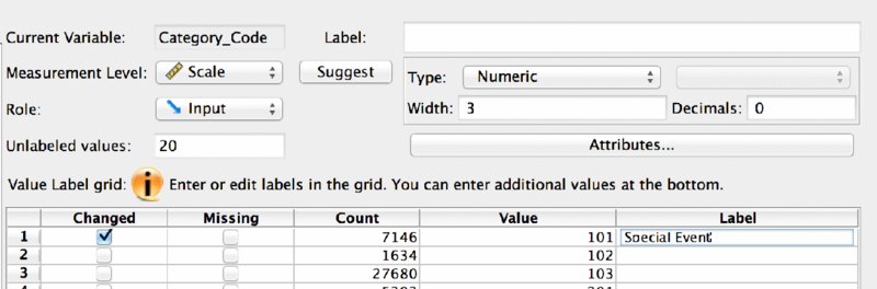
Figure 16.13 Adding a Value Label to Category_Code
The resulting syntax is quite easy to read (Figure 16.14). The FORMATS line declares Sales_Amount as Dollar, just as we indicated in the dialog. Now, we will turn our attention to completing the VALUE LABELS command.

Figure 16.14 Pasted code from the Define Variable Properties dialog
The “trick” used here is that we only pasted one of twenty one categories in the menus. The structure of the command is easily grasped, so we can imitate the structure using just that one example, supplying the relevant codes (see Figure 16.15). We simply add additional value labels. If you are lucky you might have a Word doc with these code and label pairs lying about that has been maintained by others in the organization, which would allow you to copy and paste them into the Syntax window. There is no assumption that this is another SPSS user. These product category codes tie the products with their descriptive labels so they can probably be found somewhere in electronic form. You will almost certainly have to alter the list to meet the grammatical requirements, but it will still save time.

Figure 16.15 Value Labels with additional category codes
With only twenty one codes, we wouldn’t worry about this too much, but if there were a thousand, we would ask everyone we could if the values were available in a spreadsheet somewhere before we resorted to typing. This might seem trivial, but this is just about the easiest command to learn, and there is little reason to do labeling in the menus.
Customer Dataset
Let’s take a look at the second dataset, Customer Financial Start.sav. This dataset has a variety of variables that include credit card and shipping information (all completely faked data). This represents the most recently available personal financial information for each customer, and is pulled from the most recent transaction. Much of it is unnecessary to the analysis and can be deleted, but some of the information will be important to us (Figure 16.16). In particular, we are going to rehearse three examples of formatting steps:
- Fixing the four-digit ZIP codes in Massachusetts and elsewhere
- Addressing the fact that some cities’ names are in caps, and others are not
- Parsing the e-mail addresses to place the domain name in a new variable
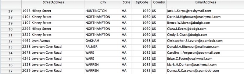
Figure 16.16 A few rows of address information in the customer data
Fixing the ZIP Codes
Our first task, fixing the ZIP codes, is straightforward enough, but will require using some conversion functions and string functions. The actual solution is a bit more involved than you might guess because SPSS doesn’t allow you to do this kind of conversion in one step. Also, the conversion is only part of the problem. We have to add (or “pad”) the zeros that are missing. We can do the first step in the windows. If you are really savvy with functions in SPSS or even Excel, you might question the creation of ZipCode2. Note the use of the Type and Label subdialog in Figure 16.17. I’m approaching it this way to make a point—a point that will become clear by the end of the example. If we paste this, we get the code shown in Lines 1–2 (Figure 16.18). We’ve already discussed that you won’t always need the DATASET ACTIVATE line that is pasted. Also, as we’ve seen, we don’t need an EXECUTE after every transformation. All of that has been removed. Note that the sidebar in the Syntax Primer section of this chapter discusses EXECUTE in some detail.
For ZipCode3, Lines 4–5, we introduce two functions, and notice that they’ve been nested. The LTRIM portion gets rid of the leading space that has filled the vacuum. We must remove that space before CHAR.LPAD can do its job of making sure that all of the ZIP codes have five characters.

Figure 16.17 Type and Label subdialog
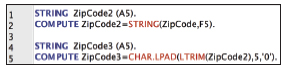
Figure 16.18 The STRING command
Now, let’s take a look at some ways to improve what was pasted. We don’t really need to keep ZipCode2. It is an intermediate step. Nesting is one way to try to address this, but in this case a very easy way is to make ZipCode2 a “scratch variable” by adding a # symbol. As a result it will never appear in the data window. It will have meaning only in the Syntax Window, and only until SPSS encounters a procedure command.
Because you can’t put string values in a numeric value, it is easier to just create a new variable and give it a meaningful name. We might have 9-digit ZIP codes for some addresses, so Zip5 seems like a good name. We no longer need the original, so we apply DELETE VARIABLES to it (Figure 16.19). We could try using RENAME VARIABLES to go back to the original if we wanted (not shown). A little documentation would be wise as well. Also, note that DELETE VARIABLES won’t execute (yet) until it is followed by a procedure command. (The difference between procedure and transformation commands is discussed in the sidebar “The Evil Execute Command” earlier in this chapter.)
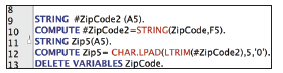
Figure 16.19 Code examples using scratch variables
Addressing Case Sensitivity of City Names with UPPER() and LOWER()
Some cities are mixed case and some are all uppercase. Why should we be concerned? A number of operations are case sensitive, including merging (it is the variable key that causes the problem) and reporting. For instance, consider the frequencies output shown in Figure 16.20. Boca Raton has 51 sales and Boise has 91, but we have to get out our scratchpad to confirm that because both cities have variation in the use of upper and lower case. Of course, there are misspellings and other issues, but we will address just the mixed case for now. It will be sufficient to accomplish our goal—identify the Top 10 cities.
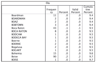
Figure 16.20 City names in mixed case
We could simply make everything all uppercase:
COMPUTE City = UPCASE(City).
But we will try a command that is a little more interesting:
COMPUTE City =
CONCAT( CHAR.SUBSTR(City,1,1) , LOWER(CHAR.SUBSTR(City,2)) ).
In theory you could work exclusively with the mouse to perform these functions, but when you are writing functions inside of functions it is easier to work in the Syntax window, and it is much easier to save your work. The new frequencies with the descending cases output shown in Figure 16.21 shows that we have made progress.

Figure 16.21 City names in descending case
We could be considerably more ambitious. For instance, “New york” has a space in its name, and we have not addressed that. It leaves the second word in its name lowercase. For this, and similar complications, we will delay a richer solution until we get to Chapter 18.
Parsing Strings and the Index Function
For this example, we are going to extract the e-mail domain information from the client’s e-mail addresses. Domains sometimes have slightly different rules on what e-mail attachments are allowed. This information might help our marketing materials successfully reach our clients. In our fake data, the e-mails are unnaturally uniform, and some of the domain names are odd, but there are plenty of formatting issues to contend with. We are only interested in the string between the @ symbol and the period that follows the @ symbol.
First we have to find the locations and the length of the domain name:
COMPUTE At_Loc=CHAR.INDEX(EmailAddress,'@').

COMPUTE Period_Loc=CHAR.RINDEX(EmailAddress,'.').

COMPUTE Domain_Length = (Period_Loc-At_Loc)-1.
Run these and examine the results. We get the locations, as an integer, of the symbols. Note that the RINDEX looks for the last instance of the period. Now, we will use the STRING and SUBSTRING functions again while converting our new variables into scratch variables:
COMPUTE #At_Loc=CHAR.INDEX(EmailAddress,'@').
COMPUTE #Period_Loc=CHAR.RINDEX(EmailAddress,'.').
COMPUTE #Domain_Length = (#Period_Loc-#At_Loc)-1.

STRING Domain(A16).
COMPUTE Domain=CHAR.SUBSTR(EmailAddress,#At_Loc+1,#Domain_Length).
EXECUTE.
This dataset is ready to merge, so we are going to switch back to the other dataset and finalize it for merging.
Aggregate and Restructure
We are almost ready to combine the datasets so we are going to switch back to the transactional dataset. We will use the Restructure Data Wizard, but for that we have to aggregate first. In a sense, this is the most sophisticated data manipulation thus far, but the menus do all the work. Take a closer look at the first customer, as shown in Figure 16.22.
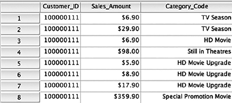
Figure 16.22 A few rows of the transactional dataset
Currently there are two lines for TV Season; restructuring forces us to have just one line. The same problem exists for HD Movie Upgrade. Aggregating easily solves the problem. We will choose both Customer_ID and Category_Code as break variables and sum customer spending within the categories. Importantly, we are using the DATASET commands for the first time. DATASET DECLARE will give our new dataset a name. This is not at all the same as saving it to a drive. If we were to exit SPSS without saving it, we would lose the new data file. When we restructure we will reference this data window by name using DATASET ACTIVATE:
DATASET DECLARE Media_Trans_AGGR.
AGGREGATE
  /OUTFILE='Media_Trans_AGGR'
  /BREAK=Customer_ID Category_Code
  /Sales_Amount_sum=SUM(Sales_Amount).
The restructure menu (see Figure 16.23) presents three choices. We want the middle choice because we want to convert a “tall dataset” into a “wide dataset.” Specifically, a transactional dataset needs to become a customer-level dataset. When you’ve made the selection, click Continue.

Figure 16.23 First screen of the Restructure Wizard
We want Customer_ID to define the height, or number of rows, of the dataset. Category_Code is in the important Index Variable Role and will define the columns of the dataset. The only variable that should be remaining, Sales_Amount_Sum will populate the body of the resulting table. See Figure 16.24. Press continue and paste the syntax.

Figure 16.24 Second screen of the Restructure Wizard
The resulting Syntax follows:
DATASET ACTIVATE Media_Trans_AGGR.
SORT CASES BY Customer_ID Category_Code.
CASESTOVARS
  /ID=Customer_ID
  /INDEX=Category_Code
  /GROUPBY=INDEX.
Pasting Variable Names, TO, Recode, and Count
Next we have to create a sum of all of our customers’ spending so that we can use it as our denominator. The menus offer up many ways to save time. We could go into the Transform ➪ Compute menu, and drag all of the variables into place, but there is also a way to be more creative. We can use just two variables to make sure that we have the proper grammar:
Compute Total_Spend = SUM( Sales_Amount_sum.101,
Sales_Amount_sum.102).
Then use the following trick. From the Utilities menu click Variables (Figure 16.25). Choose all of the variables you need, and then click Paste. The variables will appear in the Syntax window. All you have to do now is add some commas and writing the command is quite quick. You still have to understand the command, and how to write it, but you’ve saved yourself considerably on the typing.

Figure 16.25 The Utilities Menu
Compute Total_Spend = SUM( Sales_Amount_sum.101,
Sales_Amount_sum.102, Sales_Amount_sum.103,
Sales_Amount_sum.201, Sales_Amount_sum.202,
Sales_Amount_sum.203, Sales_Amount_sum.204,
Sales_Amount_sum.205, Sales_Amount_sum.301,
Sales_Amount_sum.401, Sales_Amount_sum.402,
Sales_Amount_sum.403, Sales_Amount_sum.501,
Sales_Amount_sum.502, Sales_Amount_sum.503,
Sales_Amount_sum.601, Sales_Amount_sum.701,
Sales_Amount_sum.702, Sales_Amount_sum.703,
Sales_Amount_sum.704, Sales_Amount_sum.705).
There is an even better trick we can use when we don’t have to worry about the commas. Let’s use the Count Values within Cases menu option (Figure 16.26). Located in the Transform menu, this is going to be the easiest way to determine how many null values (more accurately called “system missing” and identified with the dot in the cell) there are in our sales ratios for each customer. This will allow us to figure out how many departments they have made purchases in. Customers who shop in only one department might need a different marketing approach than those who shop in many departments. When we load the variables and Define Values as being system missing, SPSS lists all of the variables. That is OK, but our code will be easier to read if we place the TO keyword between the first and last Sales_Amount_sum variable. As an added twist, we will try a scratch variable again.

Figure 16.26 Count Values within Cases menu option
COUNT
#NumMiss=Sales_Amount_sum.101 TO Sales_Amount_sum705(SYSMIS).
Because we want to know how many departments they’ve shopped in, and not how many that they have failed to shop in, we will perform the following calculation. Now the new variable NumCats will tell us in how many sales categories they have a non-SYSMIS value:
COMPUTE NumCats = 21 - #NumMiss.
The same TO keyword can be used with the RECODE command. Note that this is the equivalent of RECODE into SAME VARIABLES in the menus because no new variable name is given. RECODE into DIFFERENT VARIABLES would require the optional INTO keyword, as shown in Figure 16.27.

Figure 16.27 RECODE command in Syntax Help
Our RECODE command will be the following:
RECODE Sales_Amount_sum.101 TO Sales_Amount_sum.705 (SYSMIS=0).
DO REPEAT Spend Ratios
We now need to create 21 ratios. We could use 21 COMPUTE statements, but we are going to use a kind of loop. The DO REPEAT command may not be familiar to you or your colleagues, but it is easily explained with just a sentence or two of documentation. It will take up less space, which makes the total code easier to read and easier to test. When a section of code is longer than a page (or a screen) it invites mistakes. We have to take 21 Numerators (one for each sales category) and divide all of them by our sum. That’s it. DO REPEAT makes it easy.
First we declare what the Command Syntax Reference calls a stand-in variable. Ours is called numerator. Using the TO keyword we can refer to all of them as long as they are contiguous—which they are. In the case of our new variables, we are going to list them all explicitly. We must because they don’t exist yet, and because the names are not a simple increment. Note that if they had names like ratio1, ratio2, and so on, we could use a code fragment like this:
ratio = ratio1 to ratio21
Because we can’t do that, we write them out explicitly, being careful to place a period at the end of this section of code. The grammar requires that we separate the declarations of the stand-ins with a slash, and terminate the section with a period.
Next we have a COMPUTE statement embedded in the middle of the command:
COMPUTE ratio = numerator / Total_Spend.
The formula uses our two stand-ins as well as our variable Total_Spend. The entire command successfully creates 21 new variables. The optional PRINT keywords display the 21 COMPUTE statements as they are actually performed by SPSS:
DO REPEAT numerator = Sales_Amount_sum.101 TO Sales_Amount_sum.705
   / ratio = Sales_Ratio.101, Sales_Ratio.102, Sales_Ratio.103,
    Sales_Ratio.201, Sales_Ratio.202, Sales_Ratio.203,
    Sales_Ratio.204, Sales_Ratio.205, Sales_Ratio.301,
    Sales_Ratio.401, Sales_Ratio.402, Sales_Ratio.403,
    Sales_Ratio.501, Sales_Ratio.502, Sales_Ratio.503,
    Sales_Ratio.601, Sales_Ratio.701, Sales_Ratio.702,
    Sales_Ratio.703, Sales_Ratio.704, Sales_Ratio.705.
COMPUTE ratio = numerator / Total_Spend.
END REPEAT PRINT.
Merge
You are likely familiar with the MERGE commands in the menus. If you have been using SPSS for a while, you might be a bit surprised by the pasted command. When you paste from the Merge menus you get the STAR JOIN command. Let’s begin in the menus. We are going to write the code to be in the Customer Financial Start dataset at the time of the merge, so we want to indicate to SPSS that we want to merge with the [Media_Trans_AGGR] dataset. Untitled9 (shown in Figure 16.28) may or may not be the filename. It is an indication of how busy a session you have had. It is not important here. What is important is the “window name”—the one that we reference with DATASET ACTIVATE and DATASET NAME.

Figure 16.28 First screen of Add Variables
In the next step, we will have an opportunity to remove some variables that we do not need. We choose Match cases on key variables, and choose Customer_ID as our key. We simply exclude Zip Code (because we’ve made a new version) and the private variables Mother’s Maiden name, CCNumber, CVV2, and NationalID (Figure 16.29).

Figure 16.29 Second screen of Add Variables
We will also paste a SAVE command into our Syntax.
Let’s briefly review some little improvements that are found in the final version. (You can find the complete program in the final section of this chapter.) Consider reviewing the final syntax file in the Syntax window where the color coding may ease your review.
- We’ve consolidated everything into one file including the GET FILE commands. These can be easily generated from the menus.
- We’ve added the FILE HANDLE command and declared both file handles at the top of the file where they can be easily changed.
- We’ve used the INSERT command, allowing the VALUE LABELS command to be stored in its own file. This can be easily updated without affecting the rest of the code.
- We’ve added a few comments for documentation. We could add even more, especially if our coworkers are new to SPSS.
There is always more to be done, but the goal of the case study was to advance your knowledge of Syntax by showing that the menus can help you assemble a single cohesive program that can perform potentially complex tasks. There are hundreds of commands to learn, but any commands that were learned were a side benefit of the primary goal: Syntax programs do not have to be stolen little bits of code. Syntax programs can be solutions to routine problems that can be documented and shared, saving you and your colleagues much time in the process.
Final Syntax File
Here is the final code in its entirety. Use this code carefully. Download the code from the book’s website. Do not attempt to type it or copy and paste it. There are three complications that make it useful for reference only, but prone to error if you are not careful.
- Embedded carraige returns can impact SPSS even when they are not visible. This is primarily a problem when there is a carraige return within quotes. Consider the first three lines of code:
FILE HANDLE Trans /NAME = '/Users/KMcCormick/Documents/Wiley SPSS
Stats/Syntax Chapter/Media Sales Transactions '+
    'Start.sav'.
The + symbol gets around this problem, but with a lengthy section of code it is easy to miss. So, again, be careful.
- Publishing has different limits for the width of code than the SPSS Syntax editor does. What fits on the line can change the appearance in a way that if imitated in the editor could cause problems. Effort has been made to minimize the effect, but in the age of electonic books and devices, it would be easy to have an error introduced by changing display column widths or font sizes.
- In a related problem, indenting code is often quite useful when writing code in the SPSS Syntax editor, but it takes up columns in print potentially exacerbating the issues listed already. In the following section (abreviated), an indent would be encouraged (as shown):
DO REPEAT numerator = Sales_Amount_sum.101 TO Sales_Amount_sum.705
    / ratio = Sales_Ratio.101, Sales_Ratio.102,
  Sales_Ratio.103, Sales_Ratio.201,
  Sales_Ratio.705.
  COMPUTE ratio = numerator / Total_Spend.
END REPEAT PRINT.
There is enough value in being able to see the “big picture,” however, that the code is listed dispite the risks. It should be able to give you a better feel for the flow of the code, especially if you are reading a traditional print book, during some stolen moments away from your laptop.
FILE HANDLE Trans /NAME = '/Users/KMcCormick/Documents/Wiley SPSS Stats/
Syntax Chapter/Media Sales Transactions '+
    'Start.sav'.

FILE HANDLE Customers /NAME='/Users/KMcCormick/Documents/
Wiley SPSS Stats/Syntax Chapter/Customer Financial Start.sav'.

FILE HANDLE Categories /NAME = '/Users/KMcCormick/Documents/
Wiley SPSS Stats/Syntax Chapter/Category Code Labels.sps'.

GET FILE = Trans.
DATASET NAME Trans WINDOW=FRONT.

* Define Variable Properties.
*Sales_Amount.
FORMATS  Sales_Amount(DOLLAR7.2).
*Category_Code.
VARIABLE LEVEL  Category_Code(NOMINAL).

* The following INSERT applies labels found in an external file.

INSERT File = Categories.

DATASET DECLARE Media_Trans_AGGR.
AGGREGATE
  /OUTFILE='Media_Trans_AGGR'
  /BREAK=Customer_ID Category_Code
  /Sales_Amount_sum=SUM(Sales_Amount).

DATASET ACTIVATE Media_Trans_AGGR.
SORT CASES BY Customer_ID Category_Code.
CASESTOVARS
  /ID=Customer_ID
  /INDEX=Category_Code
  /GROUPBY=INDEX.

Compute Total_Spend = SUM( Sales_Amount_sum.101,
Sales_Amount_sum.102, Sales_Amount_sum.103,
Sales_Amount_sum.201, Sales_Amount_sum.202,
Sales_Amount_sum.203, Sales_Amount_sum.204,
Sales_Amount_sum.205, Sales_Amount_sum.301,
Sales_Amount_sum.401, Sales_Amount_sum.402,
Sales_Amount_sum.403, Sales_Amount_sum.501,
Sales_Amount_sum.502, Sales_Amount_sum.503,
Sales_Amount_sum.601, Sales_Amount_sum.701,
Sales_Amount_sum.702, Sales_Amount_sum.703,
Sales_Amount_sum.704, Sales_Amount_sum.705).

COUNT #NumMiss=Sales_Amount_sum.101 TO Sales_Amount_sum.705(SYSMIS).

COMPUTE NumCats = 21 - #NumMiss.

RECODE Sales_Amount_sum.101 TO Sales_Amount_sum.705 (SYSMIS=0).

* ratio = ratio1 to ratio21.

DO REPEAT numerator = Sales_Amount_sum.101 TO Sales_Amount_sum.705
 / ratio = Sales_Ratio.101, Sales_Ratio.102,
 Sales_Ratio.103, Sales_Ratio.201,
 Sales_Ratio.202, Sales_Ratio.203,
 Sales_Ratio.204, Sales_Ratio.205,
 Sales_Ratio.301, Sales_Ratio.401,
 Sales_Ratio.402, Sales_Ratio.403,
 Sales_Ratio.501, Sales_Ratio.502,
 Sales_Ratio.503, Sales_Ratio.601,
 Sales_Ratio.701, Sales_Ratio.702,
 Sales_Ratio.703, Sales_Ratio.704,
 Sales_Ratio.705.
 COMPUTE ratio = numerator / Total_Spend.
END REPEAT PRINT.

Get File = Customers.

DATASET NAME Customers WINDOW=FRONT.

* Mixed Case.

COMPUTE City = CONCAT( CHAR.SUBSTR(City,1,1) ,
LOWER(CHAR.SUBSTR(City,2)) ).

* Domain Name.

COMPUTE #At_Loc=CHAR.INDEX(EmailAddress,'@').
COMPUTE #Period_Loc=CHAR.RINDEX(EmailAddress,'.').
COMPUTE #Domain_Length = (#Period_Loc-#At_Loc)-1.

STRING Domain(A16).
COMPUTE Domain=CHAR.SUBSTR(EmailAddress,#At_Loc+1,#Domain_Length).
EXECUTE.

* Zip Code.

STRING  #ZipCode2 (A5).
COMPUTE #ZipCode2=STRING(ZipCode,F5).
STRING Zip5(A5).
COMPUTE Zip5= CHAR.LPAD(LTRIM(#ZipCode2),5,'0').

STAR JOIN
  /SELECT t0.Gender, t0.GivenName, t0.MiddleInitial, t0.Surname,
t0.StreetAddress, t0.City,
t0.State, t0.Country, t0.EmailAddress, t0.TelephoneNumber, t0.Birthday,
t0.CCType, t0.CCExpires,
t0.UPS, t0.Domain, t1.Sales_Amount_sum.101,
t1.Sales_Amount_sum.102, t1.Sales_Amount_sum.103,
t1.Sales_Amount_sum.201, t1.Sales_Amount_sum.202,
t1.Sales_Amount_sum.203, t1.Sales_Amount_sum.204,
t1.Sales_Amount_sum.205, t1.Sales_Amount_sum.301,
t1.Sales_Amount_sum.401, t1.Sales_Amount_sum.402,
t1.Sales_Amount_sum.403, t1.Sales_Amount_sum.501,
t1.Sales_Amount_sum.502, t1.Sales_Amount_sum.503,
t1.Sales_Amount_sum.601, t1.Sales_Amount_sum.701,
t1.Sales_Amount_sum.702, t1.Sales_Amount_sum.703,
t1.Sales_Amount_sum.704, t1.Sales_Amount_sum.705,
t1.Total_Spend, t1.NumCats, t1.Sales_Ratio.101,
t1.Sales_Ratio.102, t1.Sales_Ratio.103,
t1.Sales_Ratio.201, t1.Sales_Ratio.202,
t1.Sales_Ratio.203, t1.Sales_Ratio.204,
t1.Sales_Ratio.205, t1.Sales_Ratio.301,
t1.Sales_Ratio.401, t1.Sales_Ratio.402,
 t1.Sales_Ratio.403, t1.Sales_Ratio.501,
t1.Sales_Ratio.502, t1.Sales_Ratio.503,
t1.Sales_Ratio.601, t1.Sales_Ratio.701,
t1.Sales_Ratio.702, t1.Sales_Ratio.703,
t1.Sales_Ratio.704, t1.Sales_Ratio.705,
    t0.Zip5
  /FROM * AS t0
  /JOIN 'Media_Trans_AGGR' AS t1
    ON t0.Customer_ID=t1.Customer_ID
  /OUTFILE FILE=*.

SAVE OUTFILE='/Users/KMcCormick/Documents/Wiley SPSS Stats
/Syntax Chapter/Syntax Chapter Complete.sav'
  /COMPRESSED.