
Chapter 6. Deducing the Best Execution Plan
For Tyme ylost may nought recovered be.
Just as reducing a word problem to abstract mathematics is usually the hardest part of solving the problem, you will usually find that producing the query diagram is harder than deducing the best execution plan from the query diagram. Now that you know the hard part, how to translate a query into a query diagram, I demonstrate the easy part. There are several questions you need to answer to fully describe the optimum execution plan for a query:
How do you reach each table in the execution plan, with a full table scan or one or more indexes, and which indexes do you use, if any?
How do you join the tables in the execution plan?
In what order do you join the tables in the execution plan?
Out of these three questions, I make a case that the only hard question, and the main point of the query diagram, is the question of join order. If you begin by finding the optimum join order, which is nearly decoupled from the other questions, you will find that answers to the other two questions are usually obvious. In the worst cases, you might need to try experiments to answer the other two questions, but these will require at most one or two experiments per table. If you did not have a systematic way to answer the join-order question, you would require potentially billions of experiments to find the best plan.
Robust Execution Plans
A subset of all possible execution plans can be described as robust. While such plans are not always quite optimum, they are almost always close to optimum in real-world queries, and they have desirable characteristics, such as predictability and low likelihood of errors during execution. (A nonrobust join can fail altogether, with an out-of-TEMP-space error if a hash or sort-merge join needs more space than is available.) Robust plans tend to work well across a wide range of likely data distributions that might occur over time or between different database instances running the same application. Robust plans are also relatively forgiving of uncertainty and error; with a robust plan, a moderate error in the estimated selectivity of a filter might lead to a moderately suboptimal plan, but not to a disastrous plan. When you use robust execution plans, you can almost always solve a SQL tuning problem once, instead of solving it many times as you encounter different data distributions over time and at different customer sites.
Tip
Uncertainty and error are inevitable in the inputs for an
optimization problem. For example, even with perfect information at
parse time (at the time the database generates the execution plan), a
condition like Last_Name = :LName
has uncertain selectivity, depending on the actual value that will be
bound to :LName at execution time.
The unavoidability of uncertainty and error makes robustness
especially important.
Robust execution plans tend to have the following properties:
Their execution cost is proportional to rows returned.
They require almost no sort or hash space in memory.
They need not change as all tables grow.
They have moderate sensitivity to distributions and perform adequately across many instances running the same application, or across any given instance as data changes.
They are particularly good when it turns out that a query returns fewer rows than you expect (when filters are more selective than they appear).
Tip
In a sense, a robust plan is optimistic: it assumes that you have designed your application to process a manageably small number of rows, even when it is not obvious how the query narrows the rowset down to such a small number.
Robustness requirements imply that you should usually choose to:
Tip
Nested loops on full join keys generally scale with the number of rows that match query conditions and avoid memory required to execute hash joins or sort-merge joins, for which memory use might turn out to be excessive. Such excessive memory use can even lead to out-of-temp-space errors if the cached rowsets turn out to be larger than you expect.
Drive down to primary keys before you drive up to nonunique foreign keys
Tip
Driving down before driving up avoids a potential explosion of rows earlier in the plan than you want when it turns out that the detail table has more details per master row than you expected.
If you consider only robust plans, robustness rules alone answer the first two questions of finding the best execution plan, leaving only the question of join order:
You will reach every table with a single index, an index on the full filter condition for the first table, and an index on the join key for each of the other tables.
You will join all tables by nested loops.
I later discuss when you can sometimes safely and profitably relax the robustness requirement for nested-loops joins, but for now I focus on the only remaining question for robust plans: the join order. I also later discuss what to do when the perfect execution plan is unavailable, usually because of missing indexes, but for now, assume you are looking for a truly optimum robust plan, unconstrained by missing indexes.
Standard Heuristic Join Order
Here is the heuristic for finding the best robust execution plan, including join order:
Drive first to the table with the best (nearest to zero) filter ratio.
With nested loops—driving through the full, unique, primary-key indexes—drive down as long as possible, first to the best (nearest to zero) remaining filters.
Only when necessary, follow nested loops up diagram links (against the direction of the arrow) through full, nonunique, foreign-key indexes.
These steps might not be perfectly clear now. Don’t worry. The rest of this chapter explains each of these steps in detail. The heuristic is almost easier to demonstrate than to describe.
When the driving table turns out to be several levels below the top detail table (the root table, so-called because it lies at the root of the join tree), you will have to return to Step 2 after every move up the tree in Step 3. I describe some rare refinements for special cases, but by and large, finding the optimum plan is that simple, once you have the query diagram!
After tuning thousands of queries from real-world applications that included tens of thousands of queries, I can state with high confidence that these rules are just complex enough. Any significant simplification of these rules will leave major, common classes of queries poorly tuned, and any addition of complexity will yield significant improvement only for relatively rare classes of queries.
Tip
Later in the book, I discuss these rarer cases and what to do with them, but you should first understand the basics as thoroughly as possible.
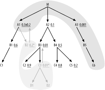
There is one subtlety to consider when Steps 2 and 3 mention following join links up or down: the tables reached in the plan so far are consolidated into a single virtual node, for purposes of choosing the next step in the plan. Alternatively, it might be easier to visualize the tables reached so far in the plan as one cloud of nodes. From the cloud of already-reached nodes, it makes no difference to the rest of the plan how already-reached table nodes are arranged within that cloud, or in what order you reached them. The answer to the question “Which table comes next?” is completely independent of the order or method you used to join any earlier tables. Which tables are in the cloud affects the boundaries of the cloud and matters, but how they got there is ancient history, so to speak, and no longer relevant to your next decision.
When you put together an execution plan following the rules, you might find yourself focused on the most-recently-joined table, but this is a mistake. Tables are equally joined upward or downward from the cloud if they are joined upward or downward from any member of the set of already-joined tables, not necessarily the most-recently-joined table. You might even find it useful to draw the expanding boundaries of the cloud of so-far-reached tables as you proceed through the steps, to clarify in your mind which tables lie just outside the cloud. The relationship of remaining tables to the cloud clarifies whether they join to the cloud from above or from below, or do not even join to the cloud directly, being ineligible to join until you join further intermediate tables. I further illustrate this point later in the chapter.
Simple Examples
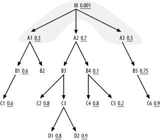
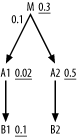
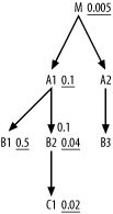
Nothing illustrates the method better than examples, so I demonstrate the method using the query diagrams built in Chapter 5, beginning with the simplest case, the two-way join, shown again in Figure 6-1.
Applying Step 1 of the method, first ask which node offers the
best (lowest) effective filter ratio. The answer is E, since E’s filter ratio of 0.1 is less than D’s ratio of 0.5. Driving from that node,
apply Step 2 and find that the best (and only) downstream node is node
D, so go to D next. You find no other tables, so that
completes the join order. Following the rules for a robust execution
plan, you would reach E with an index
on its filter, on Exempt_Flag. Then,
you would follow nested loops to the matching departments through the
primary-key index on Department_ID
for Departments. By brute force, in
Chapter 5, I already showed the
comforting result that this plan is in fact the best, at least in terms
of minimizing the number of rows touched.
Tip
The rules for robust plans and optimum robust plans take no account of what indexes you already have. Remember that this chapter addresses the question of which plan you want, and that question should not be confined by currently lacking indexes. I later address the question of settling for less than optimal plans when indexes are missing, but you must first find ideal plans before you can evaluate when to make compromises.
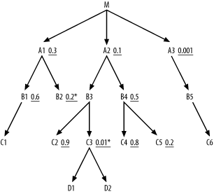
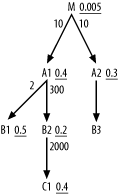
Join Order for an Eight-Way Join
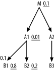
So far, so good, but two-way joins are too easy to need an elaborate new method, so let’s continue with the next example, the eight-way join. Eight tables can, in theory, be joined in 8-factorial join orders (40,320 possibilities), enough to call for a systematic method. Figure 6-2 repeats the earlier problem from Chapter 5.
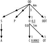
Following the heuristics outlined earlier, you can determine the optimal join order for the query diagrammed in Figure 6-2 as follows:
Find the table with the lowest filter ratio. In this case, it’s
C, with a ratio of 0.0002, soCbecomes the driving table.From
C, it is not possible to drive down to any table through a primary-key index. You must therefore move upward in the diagram.The only way up from
Cis toO, soObecomes the second table to be joined.After reaching
O, you find that you can now drive downward toOT. Always drive downward when possible, and go up only when you’ve exhausted all downward paths.OTbecomes the third table to be joined.There’s nothing below
OT, so return toOand move upward toOD, which becomes the fourth table to be joined.The rest of the joins are downward and are all unfiltered, so join to
S,P, andODTin any order.Join to
Aat any point after it becomes eligible, after the join toSplaces it within reach.
Tip
I will show that, when you consider join ratios, you will always place downward inner joins before outer joins. This is because such inner joins have at least the potential to discard rows, even in cases like this, when statistics indicate the join will have no effect on the running rowcount.
Therefore, you find the optimum join order to be C; O;
OT; OD; S,
P, and ODT in any order; and A at any point after S. This dictates 12 equally good join orders
out of the original 40,320 possibilities. An exhaustive search of all
possible join orders confirms that these 12 are equally good and are
better than all other possible join orders, to minimize rows visited
in robust execution plans.
This query diagram might strike you as too simple to represent a realistic problem, but I have found this is not at all the case. Most queries with even many joins have just one or two filters, and one of the filter ratios is usually obviously far better than any other.
For the most part, simply driving to that best filter first,
following downward joins before upward joins, and perhaps picking up
one or two minor filters along the way, preferably sooner rather than
later, is all it takes to find an excellent execution plan. That plan
is almost certainly the best or so close to the best that the
difference does not matter. This is where the simplified query
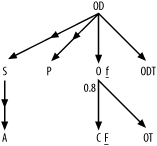
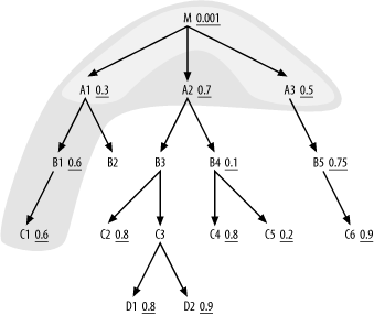
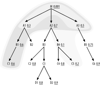
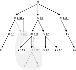
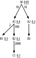
diagrams come in. The fully simplified query diagram, shown in Figure 6-3, with the best
filter indicated by the capital F
and the other filter by lowercase f, leads to the same result with only
qualitative filter information.
I will return to this example later and show that you can
slightly improve on this result by relaxing the requirement for a
fully robust execution plan and using a hash join, but for now, I
focus on teaching complete mastery of the skill of optimizing for the
best robust plan. I already showed the 12 best join orders, and I need
one of these for further illustration to complete the solution of the
problem. I choose (C, O, OT, OD, ODT, P, S, A) as the join order to
illustrate.
Completing the Solution for an Eight-Way Join
The rest of the solution is to apply the robust-plan rules to get the desired join order in a robust plan. A robust plan calls for nested loops through indexes, beginning with the filter index on the driving table and followed by indexes on the join keys. Here is the best plan in detail (refer back to Chapter 5 for the original query and filter conditions):
Drive to
Customerson an index on(Last_Name, First_Name), with a query somehow modified to make that index accessible and fully useful.Join, with nested loops, to
Orderson an index on the foreign keyCustomer_ID.Join, with nested loops, to
Code_Translations(OT) on its primary-key index(Code_Type, Code).Join, with nested loops, to
Order_Detailson an index on the foreign keyOrder_ID.Join, with nested loops, to
Code_Translations(ODT) on its primary-key index(Code_Type, Code).Outer join, with nested loops, to
Productson its primary-key indexProduct_ID.Outer join, with nested loops, to
Shipmentson its primary-key indexShipment_ID.Outer join, with nested loops, to
Addresseson its primary-key indexAddress_ID.Sort the final result as necessary.
Any execution plan that failed to follow this join order, failed
to use nested loops, or failed to use precisely the indexes shown
would not be the optimal robust plan chosen here. Getting the driving
table and index right is the key problem 90% of the time, and this
example is no exception. The first obstacle to getting the right plan
is to somehow gain access to the correct driving filter index for Step
1. In Oracle, you might use a functional index on the uppercase values
of the Last_Name and First_Name columns, to avoid the dilemma of
driving to an index with a complex expression. In other databases, you
might recognize that the name values are, or should be, always stored
in uppercase, or you might denormalize with new, indexed columns that
repeat the names in uppercase, or you might change the application to
require a case-sensitive search. There are several ways around this
specific problem, but you would need to choose the right driving table
to even discover the need.
Once you make it possible to get the driving table right, are
your problems over? Almost certainly, you have indexes on the
necessary primary keys, but good database design does not (and should
not) guarantee that every foreign key has an index, so the next likely
issue is to make sure you have foreign-key indexes Orders(Customer_ID) and Order_Details(Order_ID). These enable the
necessary nested-loops joins upward for a robust plan starting with
Customers.
Another potential problem is that optimizers might choose a join method other than nested loops to one or more of the tables, and you might need hints or other techniques to avoid the use of methods other than nested loops. If they take this course, they will likely also choose a different access method for the tables being joined without nested loops, reaching all the rows that can join at once.
Tip
However, I will show that sort-merge or hash joins to
a small table like Code_Translations would be fine here, even
slightly faster, and nearly as robust, since tables like this are
unlikely to grow very large.
In this simple case, with just the filters shown, join order is likely the least of the problems, as long as you get the driving table right and have the necessary foreign-key indexes.
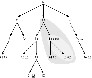
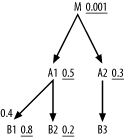
A Complex 17-Way Join
Figure 6-4 shows a deliberately complex example to fully illustrate the method. I have left off the join ratios, making Figure 6-4 a partially simplified query diagram, since the join ratios do not affect the rules you have learned so far. I will step through the solution to this problem in careful detail, but you might want to try it yourself first, to see which parts of the method you already fully understand.
For Step 1, you quickly find that B4 has the best filter ratio, at 0.001, so
choose that as the driving table. It’s best to reach such a selective
filter through an index; so, in real life, if this were an important
enough query, you might create a new index to use in driving to
B4. For now though, we’ll just
worry about the join order. Step 2 dictates that you next examine the
downward-joined nodes C4 and
C5, with a preference to join to
better-filtered nodes first. C5 has
a filter ratio of 0.2, while C4 has
a filter ratio of 0.5, so you join to C5 next. At this point, the beginning join
order is (B4, C5), and the cloud
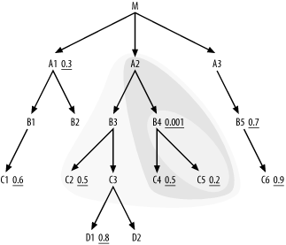
around the so-far-joined tables looks like Figure 6-5.
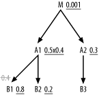
If C5 had one or more nodes
connected below, you would now have to compare them to C4, but since it does not, Step 2 offers
only the single choice of C4. When
you widen the cloud boundaries to include C4, you find no further nodes below the
cloud, so you move on to Step 3, find the single node A2 joining the cloud from above, and add it
to the building join order, which is now (B4,
C5, C4, A2). The cloud around the so-far-joined tables now
looks like Figure
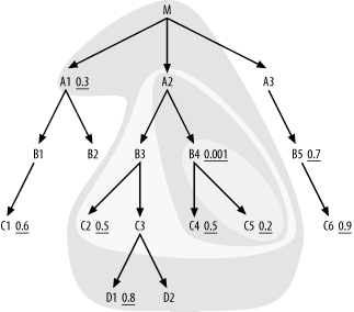
6-6.
Note that I left in the original two-node cloud in gray. In
practice, you need not erase the earlier clouds; just redraw new
clouds around them. Returning to Step 2, find downstream of the
current joined-tables cloud a single node, B3, so put it next in the join order without
regard to any filter ratio it might have. Extend the cloud boundaries
to include B3, so you now find
nodes C2 and C3 applicable under Step 2, and choose
C2 next in the join order, because
its filter ratio of 0.5 is better than the implied filter ratio of 1.0
on unfiltered C3. The join order so
far is now (B4, C5, C4, A2, B3, C2). Extend the cloud further around
C2. This brings no new downstream
nodes into play, so Step 2 now offers only C3 as an alternative. The join order so far
is now (B4, C5, C4, A2, B3, C2,
C3), and Figure
6-7 shows the current join cloud.
Step 2 now offers two new nodes below the current join cloud,
D1 and D2, with D1 offering the better filter ratio. Since
neither of these has nodes joined below, join to them in filter-ratio
order and proceed to Step 3, with the join order so far now (B4, C5, C4, A2,
B3, C2, C3, D1, D2). This completes the entire branch from
A2 down, leaving only the upward
link to M (the main table being
queried) to reach the rest of the join tree, so Step 3 takes you next
to M. Since you have reached the
main table at the root of the join tree, Step 3 does not apply for the
rest of the problem. Apply Step 2 until you have reached the rest of
the tables. Immediately downstream of M (and of the whole join cloud so far), you
find A1 and A3, with only A1 having a filter, so you join to A1 next. Now, the join order so far is
(B4, C5, C4, A2, B3, C2, C3, D1,
        D2
, M, A1), and Figure 6-8 shows the current
join cloud.
Find immediately downstream of the join cloud nodes B1, B2,
and A3, but none of these have
filters, so look for two-away filters that offer the best filter
ratios two steps away. You find such filters on C1 and B5, but C1 has the best, so add B1 and C1
to the running join order. Now, the join order so far is (B4, C5, C4, A2, B3, C2, C3, D1, D2, M, A1, B1, C1). You still find no better
prospect than the remaining two-away filter on B5, so join next to A3 and B5, in that order. Now, the only two nodes
remaining, B2 and C6, are both eligible to join next, being
both directly attached to the join cloud. Choose C6 first, because it has a filter ratio of
0.9, which is better than the implied filter ratio of 1.0 for the
unfiltered join to B2. This
completes the join order:(B4, C5, C4, A2, B3,
C2, C3, D1, D2, M, A1, B1, C1, A3, B5, C6, B2).
Apart from the join order, the rules specify that the database
should reach table B4 on the index
for its filter condition and the database should reach all the other
tables in nested loops to the indexes on their join keys. These
indexed join keys would be primary keys for downward joins to C5, C4,
B3, C2, C3,
D1, D2, A1,
B1, C1, A3,
B5, C6, and B2, and foreign keys for A2 (pointing to B4) and M
(pointing to A2). Taken together,
this fully specifies a single optimum robust plan out of the
17-factorial (355,687,428,096,000) possible join orders and all
possible join methods and indexes. However, this example is artificial
in two respects:
Real queries rarely have so many filtered nodes, so it is unlikely that a join of so many tables would have a single optimum join order. More commonly, there will be a whole range of equally good join orders, as I showed in the previous example.
The later part of the join order matters little to the runtime, as long as you get the early join order right and reach all the later tables through their join keys. In this example, once the database reached node
M, and perhapsA1, with the correct path, the path to the rest of the tables would affect the query runtime only slightly. In most queries, even fewer tables really matter to the join order, and often you will do fine with just the correct driving table and nested loops to the other tables following join keys in any order that the join tree permits.
Tip
If you need to change a query anyway and have the chance to get the whole join order right, you might as well. However, if you already have a plan that is correct in the early join order, the improvement might not be worth the trouble of changing the query just to change the end of the join order.
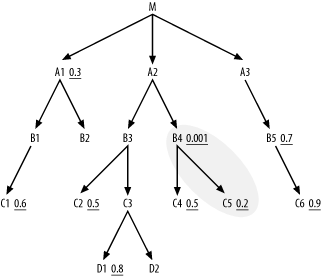
A Special Case
Usually, following the tuning-process steps without deviation works fine, but the problem shown in Figure 6-4 turns out to offer, potentially, one last trick you could apply, especially with Oracle.
Tip
This section first describes an especially efficient trick that sometimes helps on Oracle. However, take heart if you need something like this outside of Oracle: at the end of the section, I describe a less efficient version of the trick for other databases.
The Oracle Solution
Return to Figure
6-4 and consider a special case: all tables other than M are relatively small and well cached, but
M is very large and therefore
poorly cached and much more expensive to access than the other tables.
Furthermore, M is a special
combinations table to express a many-to-many
relationship between A1 and
A2. An example of such a
combinations table would be a table of actor/movie combinations for a
movie-history database, linking Movies and Actors, when the relationship between these
is many-to-many. In such a combinations table, it is natural to use a
two-part primary key made up of the IDs of the linked tables—in this
case, Movie_ID and Actor_ID. As is commonly the case, this
combinations table has an index on the combination of foreign keys
pointing to the tables A2 and
A1. For this example, assume the
order of the keys within that index has the foreign key pointing to
A2 first, followed by the foreign
key pointing to A1 .
Consider the costs of accessing each table in the plan I found
earlier as the original solution to Figure 6-4. You find low costs
for the tables up to M, then a much
higher cost for M because you get
many more rows from that table than the previous tables and accessing
those rows leads to physical I/O. Following M, the database joins to just as many rows
in A1 (since M has no filter), but these are much cheaper
per row, because they are fully cached. Then, the filter in A1 drops the rowcount back down to a much
lower number for the remaining tables in the plan. Therefore, you find
a cost almost wholly dominated by the cost of accessing M, and it would be useful to reduce that
cost.
As it happens, in this unusual case, you find an opportunity to
get from the foreign key in M
pointing to A2 to the foreign key
pointing to A1, stored in the same
multicolumn index in M, without
ever touching the table M! The
database will later need to read rows from the table itself, to get
the foreign key pointing to A3 and
probably to get columns in the query SELECT list. However, you can postpone going
to the table until after the database reaches filtered tables A1 and C1. Therefore, the database will need to go
only to 18% as many rows in M (0.3
/ 0.6, picking up the filter ratios 0.3 on A1 and 0.6 on C1) as it would need to read if the database
went to the table M as soon as it
went to the index for M. This
greatly reduces the query cost, since the cost of reading rows in
table M, itself, dominates in this
particular case.
No database makes it particularly easy to decouple index reads
from table reads; a table read normally follows an index read
immediately, automatically, even when this is not optimal. However,
Oracle does allow for a trick that solves the problem, since Oracle
SQL can explicitly reference rowids. In this case, the best join order
is (B4, C5, C4, A2, B3, C2, C3, D1, D2, MI,
A1, B1, C1, MT, A3, B5, C6, B2). Here, MI is the index on M(FkeyToA2,FkeyToA1), inserted into the join
order where M was originally.
MT is the table M, accessed later in the plan through the
ROWID from MI and inserted into the join order after
picking up the filters on A1 and
C1. The trick is to refer to
M twice in the FROM clause, once for the index-only access
and once for a direct ROWID join,
as follows, assuming that the name of the index on M(FkeyToA2,FkeyToA1) is M_DoubleKeyInd:
Select /*+ ORDERED INDEX(MI M_DoubleKeyInd) */ MT.Col1, MT.Col2,...
...
FROM B4, C5, C4, A2, B3, C2, C3, D1, D2,
M MI, A1, B1, C1, M MT, A3, B5, C6, B2
WHERE ...
AND A2.Pkey=MI.FKeyToA2
AND A1.Pkey=MI.FKeyToA1
AND MI.ROWID=MT.ROWID
AND...
So, two joins to M are really
cheaper than one in this unusual case! Note the two hints in this
version of the query:
ORDEREDSpecifies that the tables are to be joined in the order they occur in the
FROMclauseINDEX(MI M_DoubleKeyInd)Guarantees use of the correct index at the point in the order where you want index-only access for
MI
Other hints might be necessary to get the rest of the plan just
right. Also note the unusual rowid-to-rowid join between MI and MT, and note that the only references to
MI are in the FROM clause and in the WHERE clause conditions shown. These
references require only data (the two foreign keys and the rowid)
stored in the index. This is crucial: Oracle avoids going to the table
M as soon as it reaches the index
on the primary key to M only
because MI refers solely to the
indexed columns and the rowids that are also stored in the index.
Columns in the SELECT clause and
elsewhere in the WHERE-clause
conditions (such as a join to A3,
not shown) all come from MT.
Because of all this, the optimizer finds that the only columns
required for MI are already
available from the index. It counts that join as index-only. The
direct-ROWID join to MT occurs later in the join order, and any
columns from the M table are
selected from MT.
However, the technique I’ve just described is not usually needed, for several reasons:
Combination indexes of the two foreign keys you need, in the right order you need, happen rarely.
Usually, the root detail table does not add enough cost, in both relative and absolute terms, to justify the trouble.
The benefits rarely justify creating a whole new multicolumn index if one is not already there.
Solving the Special Case Outside of Oracle
If you cannot refer directly to rowids in your WHERE clause, can this trick still work in
some form? The only part of the trick that depends on rowids is the
join between MI and MT. You could also join those table aliases
on the full primary key. The cost of the early join to MI would be unchanged, but the later join to
MT would require looking up the
very same index entry you already reached in the index-only join to
MI for those rows that remain. This
is not as efficient, but note that these redundant hits on the index
will surely be cached, since the execution plan touches the same index
entries moments before, leaving only the cost of the extra logical
I/O. Since the database throws most of the rows out before it even
reaches MT, this extra logical I/O
is probably much less than the savings on access to the table
itself.
A Complex Example
Now, I demonstrate an example that delivers a less straightforward join order that requires more attention to the whole join cloud. You will find that the sequence of next-best tables can jump all over the query diagram in cases like the one I describe in this section. Consider the problem in Figure 6-9, and try it yourself before you read on.
Here, you see, as is quite common, that the best filter falls on the root detail table.
Tip
The best filter is often on the root detail table, because the entities of this table are the true focus of the query. It is common that the main filter references a direct property of those entities, rather than some inherited property in the joined tables.
Since you will drive from the root detail table, Step 3 will never apply; you have no nodes upstream of the starting point. The cloud of tables joined so far will grow downward from the top, but keep in mind that you can find the next-best node anywhere along the boundary of this cloud, not necessarily near the last table joined. Try to find the best join order yourself before you read on.
The first eligible nodes are A1, A2, and
A3, and the best filter ratio lies on
A1, so A1 falls second in the join order. After
extending the join cloud to A1, add
B1 and B2 to the eligible nodes, and A2 and A3
are still eligible. Between these four nodes, A3 has the best filter ratio, so join to it
next. The join order, so far, is (M, A1,
A3), and the join cloud now looks like Figure 6-10.
The list of eligible nodes attached to the join cloud is now
B1, B2, A2, and
B5. B1 has the best filter ratio among these, so
join to it next, extending the cloud and adding C1 to the list of eligible nodes, which is now
B2, A2, B5, and
C1. Among these, C1 is the best, so join to it next and extend
the cloud further. C1 has no
downstream nodes, so proceed to the next-best node on the current list,
A2, which adds B3 and B4
to the list of eligible nodes, which is now B2, B5,
B3, and B4. The join order, so far, is (M, A1, A3, B1, C1,
A2), and the join cloud now looks like Figure 6-11.
Among the eligible nodes, B4
has, by far, the best filter ratio, so it comes next. (It would have
been great to join to it earlier, but it did not become eligible until
the database reached A2.) The join
order to B4 adds C4 and C5
to the eligible list, which now includes B2, B5,
B3, C4, and C5.
Of these, C5 is by far the best, so
it comes next. The join order, so far, is (M,
A1, A3, B1, C1, A2, B4, C5), and the join cloud now looks like
Figure 6-12.
Eligible nodes attached below the join cloud now include B2, B3,
B5, and C4, and the best filter among these is
B5. B5 adds C6
to the eligible list, and the next-best on the list is C4, which adds no new node to the list.
C6 is the next-best node, but it also
adds no new node to the eligible-nodes list, which is now just B2 and B3.
Neither of these even has a filter, so you look for two-away filters and
find that B3 at least gives access to
the filter on C2, so you join to
B3 next. The join order, so far, is
(M, A1, A3, B1, C1, A2, B4, C5, B5, C4, C6, B3), and the
join cloud now looks like Figure
6-13.
You now find eligible nodes B2,
C2, and C3, and only C2 has a filter, so join to C2 next. It has no downstream node, so choose
between B2 and C3 and again use the tiebreaker that C3 at least gives access to two-away filters
on D1 and D2, so join C3 next. The join order, so far, is now
(M, A1, A3, B1, C1, A2, B4, C5, B5, C4, C6, B3,
      C2
, C3). The eligible
downstream nodes are now B2, D1, and D2.
At this point in the process, the eligible downstream nodes are the only
nodes left, having no nodes further downstream. Just sort the nodes left
by filter ratio, and complete the join order: (M, A1, A3, B1, C1,
A2, B4, C5, B5, C4, C6, B3, C2, C3, D1, D2, B2). In real
queries, you usually get to the point of just sorting immediately
attached nodes sooner. In the common special case of a single detail
table with only direct joins to master-table lookups (dimension tables,
usually), called a star join, you sort master nodes
right from the start.
Given the optimal order just derived, complete the specification
of the execution plan by calling for access to the driving table
M from an index for the filter
condition on that table. Then join the other tables using nested loops
joins that follow indexes on those tables’ primary keys.
Special Rules for Special Cases
The heuristic rules so far handle most cases well and nearly always generate excellent, robust plans. However, there are some assumptions behind the rationale for these rules, which are not always true. Surprisingly often, even when the assumptions are wrong, they are right enough to yield a plan that is at least close to optimum. Here, I lay these assumptions out and examine more sophisticated rules to handle the rare cases in which deviations from the assumptions matter:
Intermediate query results in the form of Cartesian products lead to poor performance. If you do not follow the joins when working out a join order, the result is a Cartesian product between the first set of rows and the rows from the leaped-to node. Occasionally, this is harmless, but even when it is faster than a join order following the links, it is usually dangerous and scales poorly as table volumes increase.
Detail join ratios are large, much greater than 1.0. Since master join ratios (downward on the join tree) are never greater than 1.0, this makes it much safer to join downward as much as possible before joining upward, even when upward joins give access to more filters. (The filters on the higher nodes usually do not discard more rows than the database picks up going to the more detailed table.) Even when detail join ratios are small, the one-to-many nature of the join offers at least the possibility that they could be large in the future or at other sites running the same application. This tends to favor SQL that is robust for the case of a large detail join ratio, except when you have high confidence that the local, current statistics are relatively timeless and universal.
The table at the root of the join tree is significantly larger than the other tables, which serve as master tables or lookup tables to it. This assumption follows from the previous assumption. Since larger tables have poorer hit ratios in cache and since the rowcount the database reads from this largest table is often much larger than most or all other rowcounts it reads, the highest imperative in tuning the query is to minimize the rowcount read from this root detail table.
Master join ratios are either exactly 1.0 or close enough to 1.0 that the difference doesn’t matter. This follows in the common case in which detail tables have nonnull foreign keys with excellent referential integrity.
When tables are big enough that efficiency matters, there will be one filter ratio that is much smaller than the others. Near-ties, two tables that have close to the same filter ratio, are rare. If the tables are large and the query result is relatively small, as useful query results almost always are, then the product of all filter ratios must be quite small. It is much easier to get this small result with one selective filter, sometimes combined with a small number of fairly unselective filters, than with a large number of comparable, semiselective filters. Coming up with a business rationale for lots of semiselective filters turns out to be difficult, and, empirically speaking, I could probably count on one hand the number of times I’ve seen such a case in over 10 years of SQL tuning. Given one filter that is much more selective than the rest, the way to guarantee reading the fewest rows from that most important root detail table is to drive the query from the table with that best filter.
The rowcount that the query returns, even before any possible aggregation, will be small enough that, even for tiny master tables, there is little or no incentive to replace nested loops through join keys with independent table reads followed by hash joins. Note that this assumption falls apart if you do the joins with a much higher rowcount than the query ultimately returns. However, the heuristics are designed to ensure that you almost never find a much higher rowcount at any intermediate point in the query plan than the database returns from the whole query.
The following sections add rules that handle rare special cases that go against these assumptions.
Safe Cartesian Products
Consider the query diagrammed in Figure 6-14. Following the
usual rules (and breaking ties by choosing the leftmost node, just for
consistency), you drive into the filter on T1 and join to M following the index on the foreign key
pointing to T1. You then follow the
primary-key index into T2,
discarding in the end the rows that fail to match the filter on
T2. If you assume that T1 has 100 rows, based on the join ratios
M must have 100,000 rows and
T2 must have 100 rows.

The plan just described would touch 1 row in T1, 1,000 rows in M (1% of the total), and 1,000 rows in
T2 (each row in T2 10 times, on average), before discarding
all but 10 rows from the result. Approximating query cost as the
number of rows touched, the cost would be 2,001. However, if you broke
the rules, you could get a plan that does not follow the join links.
You could perform nested loops between T1 and T2, driving into their respective filter
indexes. Because there is no join between T1 and T2
the result would be a Cartesian product of all rows that meet the
filter condition on T1 and all rows
that meet the filter condition on T2. For the table sizes given, the resulting
execution plan would read just a single row from each of T1 and T2. Following the Cartesian join of T1 and T2, the database could follow an index on
the foreign key that points to T1,
into M, to read 1,000 rows from
M. Finally, the database would
discard the 990 rows that fail to meet the join condition that matches
M and T2.
Tip
When you skip using a join condition at every step of the query, one of the joins ends up left over, so to speak, never having been used for the performance of a join. The database later discards rows that fail to match the leftover join condition, effectively treating that condition as a filter as soon as it reaches both tables the join references.
Using the Cartesian product, the plan costs just 1,002, using the rows-touched cost function.
What happens if the table sizes double? The original plan cost,
following the join links, exactly doubles, to 4,002, in proportion to
the number of rows the query will return, which also doubles. This is
normal for robust plans, which have costs proportional to the number
of rows returned. However, the Cartesian-product plan cost is less
well behaved: the database reads 2 rows from T1; then, for each of those rows, reads the
same 2 rows of T2 (4 rows in all);
then, with a Cartesian product that has 4 rows, reads 4,000 rows from
M. The query cost, 4,006, now is
almost the same as the cost of the standard plan. Doubling table sizes
once again, the standard plan costs 8,004, while the Cartesian-product
plan costs 16,020. This demonstrates the lack of robustness in most
Cartesian-product execution plans, which fail to scale well as tables
grow. Even without table growth, Cartesian-product plans tend to
behave less predictably than standard plans, because filter ratios are
usually averages across the possible values. A filter that matches
just one row on average might sometimes match 5 or 10 rows for some
values of the variable. When a filter for a standard, robust plan is
less selective than average, the cost will scale up proportionally
with the number of rows the query returns. When a Cartesian-product
plan runs into the same filter variability, its cost might scale up as
the square of the filter variability, or worse.
Sometimes, though, you can have the occasional advantages of Cartesian products safely. You can create a Cartesian product of as many guaranteed-single-row sets as you like with perfect safety, with an inexpensive, one-row result. You can even combine a one-row set with a multirow set and be no worse off than if you read the multirow set in isolation from the driving table. The key advantage of robust plans is rigorous avoidance of execution plans that combine multiple multirow sets. You might recall that in Chapter 5 the rules required you to place an asterisk next to unique filter conditions (conditions guaranteed to match at most a single row). I haven’t mentioned these asterisks since, but they finally come into play here.
Consider Figure
6-15. Note that you find two unique filters, on B2 and C3. Starting from the single row of C3 that matches its unique filter condition,
you know it will join to a single row of D1 and D2, through their primary keys, based on the
downward-pointing arrows to D1 and
D2. Isolate this branch, treating
it as a separate, single-row query. Now, query the single row of
B2 that matches its unique filter
condition, and combine these two independent queries by Cartesian
product for a single-row combined set.
Placing these single-row queries first, you find an initial join
order of (C3, D1, D2, B2) (or (B2, C3,
D1, D2); it makes no difference). If you think of this
initial prequeried single-row result as an independent operation, you
find that tables A1 and B3 acquire new filter conditions, because
you can know the values of the foreign keys that point to B2 and C3
before you perform the rest of the query. The modified query now looks
like Figure 6-16, in
which the already-executed single-row queries are covered by a gray
cloud, showing the boundaries of the already-read portion of the
query.
Upward-pointing arrows show that the initial filter condition on
A1 combines with a new filter
condition on the foreign key into B2 to reach a combined selectivity of 0.06,
while the initially unfiltered node B3 acquires a filter ratio of 0.01 from its
foreign-key condition, pointing into C3.
Warning
Normally, you can assume that any given fraction of a master
table’s rows will join to about the same fraction of a detail
table’s rows. For transaction tables, such as Orders and Order_Details, this is a good assumption.
However, small tables often encode types or statuses, and the
transaction tables usually do not have evenly distributed types or
statuses. For example, with a five-row status table (such as
B2 might be), a given status
might match most of the transaction rows or almost none of them,
depending on the status. You need to investigate the actual, skewed
distribution in cases like this, when the master table encodes
asymmetric meanings.
You can now optimize the remaining portion of the query, outside
the cloud, exactly as if it stood alone, following the standard rules.
You then find that A3 is the best
driving table, having the best filter ratio. (It is immaterial that
A3 does not join directly to
B2 or C3, since a Cartesian product with the
single-row set is safe.) From there, drive down to B5 and C6, then up to M. Since A1 acquired added selectivity from its
inherited filter on the foreign key that points to B2, it now has a better filter ratio than
A2, so join to A1 next. So far, the join order is (C3, D1, D2, B2, A3, B5, C6, M, A1), and the
query, with a join cloud, looks like Figure 6-17.
Since you preread B2, the
next eligible nodes are B1 and
A2, and A2 has the better filter ratio. This adds
B3 and B4 to the eligible list, and you find that
the inherited filter on B3 makes it
the best next choice in the join order. Completing the join order,
following the normal rules, you reach B4, C5,
B1, C4, C2,
and C1, in that order, for a
complete join order of (C3, D1, D2, B2, A3,
B5, C6, M, A1, A2, B3, B4, C5, B1, C4, C2, C1).
Even if you have just a single unique filter condition, follow this process of prereading that single-row node or branch, passing the filter ratio upward to the detail table above and optimizing the resulting remainder of the diagram as if the remainder of the diagram stood alone. When the unique condition is on some transaction table, not some type or status table, that unique condition will also usually yield the best filter ratio in the query. In this case, the resulting join order will be the same order you would choose if you did not know that the filter condition was unique. However, when the best filter is not the unique filter, the best join order can jump the join skeleton, which is to say that it does not reach the second table through a join key that points to the first table.
Detail Join Ratios Close to 1.0
Treat upward joins like downward joins when the join ratio is close to 1.0 and when this allows access to useful filters (low filter ratios) earlier in the execution plan. When in doubt, you can try both alternatives. Figure 6-18 shows a case of two of the upward joins that are no worse than downward joins. Before you look at the solution, try working it out yourself.

As usual, drive to the best filter, on B4, with an index, and reach the rest of the
tables with nested loops to the join-key indexes. Unlike previous
cases, you need not complete all downward joins before considering to
join upward with a join ratio equal to 1.0.
Tip
These are evidently one-to-many joins that are nearly always one-to-one, or they are one-to-zero or one-to-many, and the one-to-zero cases cancel the row increase from the one-to-many cases. Either way, from an optimization perspective they are almost the same as one-to-one joins.
As usual, look for filters in the immediately adjacent nodes
first, and find that the first two best join opportunities are
C5 and then C4. Next, you have only the opportunity for
the upward join to unfiltered node A2, which you would do next even if the
detail join ratio were large. (The low join ratio to A2 turned out not to matter.) So far, the
join order is (B4, C5, C4,
A2).
From the cloud around these nodes, find immediately adjacent
nodes B3 (downward) and M (upward). Since the detail join ratio to
M is 1.0, you need not prefer to
join downward, if other factors favor M. Neither node has a filter, so look at
filters on nodes adjacent to them to break the tie. The best filter
ratio adjacent to M is 0.3 (on
A1), while the best adjacent to
B3 is 0.5 (on C2), favoring M, so join next to M and A1.
The join order at this point is (B4, C5, C4,
A2, M, A1). Now that the database has reached the root node,
all joins are downward, so the usual rules apply for the rest of the
optimization, considering immediately adjacent nodes first and
considering nodes adjacent to those nodes to break ties. The complete
optimum join order is (B4, C5, C4, A2, M, A1,
B3, C2, B1, C1, A3, B5, C6, C3, D1, (D2, B2)).
Tip
Here, the notation (B2, D2)
at the end of the join order signifies that the order of these last
two does not matter.
Note that, even in this specially contrived case designed to
show an exception to the earlier rule, you find only modest
improvement for reaching A1 earlier
than the simple heuristics would allow, since the improvement is
relatively late in the join order.
Join Ratios Less than 1.0
If either the detail join ratio or the master join ratio is less than 1.0, you have, in effect, a join that is, on average, [some number]-to-[less than 1.0]. Whether the less-than-1.0 side of that join is capable of being to-many is immaterial to the optimization problem, as long as you are confident that the current average is not likely to change much on other database instances or over time. If a downward join with a normal master join ratio of 1.0 is preferred over a to-many upward join, a join that follows a join ratio of less than 1.0 in any direction is preferred even more. These join ratios that are less than 1.0 are, in a sense, hidden filters that discard rows when you perform the joins just as effectively as explicit single-node filters discard rows, so they affect the optimal join order like filters.
Rules for join ratios less than 1.0
You need three new rules to account for the effect of smaller-than-normal join ratios on choosing the optimum join order:
When choosing a driving node, all nodes on the filtered side of a join inherit the extra benefit of the hidden join filter. Specifically, if the join ratio less than 1.0 is J and the node filter ratio is R, use J x R when choosing the best node to drive the query. This has no effect when comparing nodes on the same side of a join filter, but it gives nodes on the filtered side of a join an advantage over nodes on the unfiltered side of the join.
When choosing the next node in a sequence, treat all joins with a join ratio J (a join ratio less than 1.0) like downward joins, and use J x R as the effective node filter ratio when comparing nodes, where R is the single-node filter ratio of the node reached through that filtering join.
However, for master join ratios less than 1.0, consider whether the hidden filter is better treated as an explicit foreign-key-is-not-null filter. Making the is-not-null filter explicit allows the detail table immediately above the filtering master join also to inherit the adjusted selectivity J x R for purposes of both choice of driving table and join order from above. See the following sections for more details on this rule.
Detail join ratios less than 1.0
The meaning of the small join ratio turns out to be
quite different depending on whether it is the master join ratio or
the detail join ratio that is less than 1.0. A detail join ratio
less than 1.0 denotes the possibility of multiple details, when it
is more common to have no details of that particular type than to
have more than one. For example, you might have an Employees table linked to a Loans table to track loans the company
makes to a few top managers as part of their compensation. The
database design must allow for some employees to have multiple
loans, but far more employees have no loans from the company at all,
so the detail join ratio would be nearly 0. For referential
integrity, the Employee_ID column
in Loans must point to a real
employee; that is its only purpose, and all loans in this table are
to employees. However, there is no necessity at all for an Employee_ID to correspond to any loan. The
Employee_ID column of Employees exists (like any primary key) to
point to its own row, not to point to rows in another table, and
there is no surprise when the join fails to find a match in the
upward direction, pointing from primary key to foreign key.
Since handling of detail join ratios less than 1.0 turns out
to be simpler, though less common, I illustrate that case first.
I’ll elaborate the example of the previous paragraph to try to lend
some plausibility to the new rules. Beginning with a query that
joins Employees to Loans, add a join to Departments, with a filter that removes
half the departments. The result is shown in Figure 6-19, with each node
labeled by the initial of its table.
Tip
Note that Figure
6-19 shows 1.0 as the filter ratio for L, meaning that L has no filter at all. Normally, you
leave out filter ratios equal to 1.0. However, I include the
filter ratio on L to make clear
that the number 0.01 near the top of the link to L is the detail join ratio on the link
from E to L, not the filter ratio on L.
Let there be 1,000 employees, 10 departments, and 10 loans to
8 of those employees. Let the only filter be the filter that
discards half the departments. The detail join ratio to Loans must be 0.01, since after joining
1,000 employees to the Loans
table, you would find only the 10 loans. The original rules would
have you drive to the only filtered table, Departments, reading 5 rows, joining to
half the employees, another 500 rows, then joining to roughly half
the loans (from the roughly 4 employees in the chosen half of the
departments). The database would then reach 5 loans, while
performing 496 unsuccessful index range scans on the Employee_ID index for Loans using Employee_IDs of employees without
loans.
On the other hand, if the Loans table inherits the benefit of the
filtering join, you would choose to drive from Loans, reading all 10 of them, then go to
the 10 matching rows in Employees
(8 different rows, with repeats to bring the
total to 10). Finally, join to Departments 10 times, when the database
finally discards (on average) half. Although the usual objective is
to minimize rows read from the top table, this example demonstrates
that minimizing reads to the table on the upper end of a strongly
filtering detail join is nowhere near as important as minimizing
rows read in the much larger table below it.
How good would a filter on Employees have to be to bring the rows
read from Employees down to the
number read in the second plan? The filter would have to be exactly
as good as the filtering join ratio, 0.01. Imagine that it were even
better, 0.005, and lead to just 5 employees (say, a filter on
Last_Name). In that case, what
table should you join next? Again, the original rules would lead you
to Departments, both because it
is downward and because it has the better filter ratio. However,
note that from 5 employees, the database will reach, on average,
just 0.05 loans, so you are much better off joining to Loans before joining to Departments.
Tip
In reality, the end user probably chose a last name of one
of those loan-receiving employees, making these filters more
dependent than usual. However, even in that case, you would
probably get down to one or two loans and reduce the last join to
Departments to a read of just
one or two rows, instead of five.
Optimizing detail join ratios less than 1.0 with the rules
Figure 6-20 illustrates another example with a detail join ratio under 1.0. Try working out the join order before you read on.
First, examine the effect of the join ratio on the choice of
driving table. In Figure
6-21, I show the adjustments to filter ratios from the
perspective of choosing the driving table. After these adjustments,
the effective filter of 0.003 on M is best, so drive from M. From this point, revert to the original
filter ratios to choose the rest of the join order, because, when
driving from any node (M,
A2, or B2) on the detail side of that join, this
join ratio no longer applies. In a more complex query, it might seem
like a lot of work to calculate all these effective filter values
for many nodes on one side of a filtering join. In practice, you
just find the best filter ratio on each side (0.01 for A1 and 0.03 for M, in this case) and make a single
adjustment to the best filter ratio on the filtered side of the
join.
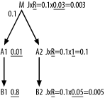
Tip
If the join ratio has a single, constant effect throughout the query optimization, you can simply fold that effect into the filter ratios, but the effect changes as optimization proceeds, so you have to keep these numbers separate.
When choosing the rest of the join order, compare the original
filter ratios on A1 and A2, and choose A1 next. Comparing B1 to A2, choose B1, and find the join order so far:
(M, A1, B1). The rest of the join
order is fully constrained by the join skeleton, for a complete join
order of (M, A1, B1, A2,
B2).
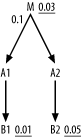
Figure 6-22
leads to precisely the same result. It makes no difference that this
time the lowest initial filter ratio is not directly connected to
the filtering join; all nodes on the filtered side of the join get
the benefit of the join filter when choosing the driving table, and
all nodes on the other side do not. Neither A1 nor A2 offers filters that drive from M, so choose A1 first for the better two-away filter on
B1, and choose the same join
order as in the last example.
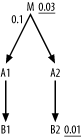
In Figure 6-23,
M and B2 get the same benefit from the filtering
join, so simply compare unadjusted filter ratios and choose B2. From there, the join order is fully
constrained by the join skeleton: (B2, A2,
M, A1, B1).
In Figure 6-24, again you compare only filtered nodes on the same side of the filtering join, but do you see an effect on later join order?
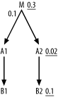
The benefit of the filtering join follows only if you follow
the join in that direction. Since you drive from A2, join to M with an ordinary one-to-many join from
A2, which you should postpone as
long as possible. Therefore, join downward to B2 before joining upward to M, even though M has the better filter ratio. The join
order is therefore (A2, B2, M, A1,
B1).
Try working out the complete join order for Figure 6-25 before you read on.
Here, note that the adjustment to filter ratios when choosing
the driving table is insufficient to favor the filtered side of the
join; the best filter on A1 is
still favored. Where do you go from there, though? Now, the
filtering join does matter. This theoretically one-to-many join is
really usually one-to-zero, so, even though it is upward on the
diagram, you should favor it over an ordinary downward join with a
normal join ratio (unshown, by convention) of 1.0. For purposes of
choosing the next table, the effective filter on M is R /
J (0.3 / 0.1=0.03), better than the filter on
B1, so join to M next. However, when you compare A2 and B1, compare simple, unadjusted filter
ratios, because you have, in a sense, already burned the benefit of
the filtering join to M. The full
join order, then, is (A1, M, B1, A2,
B2).
Master join ratios less than 1.0
Master join ratios less than 1.0 have two potential explanations:
The relationship to the master does not apply (or is unknown) in some cases, where the foreign key to that master is null.
The relationship to the master table is corrupt in some cases, where the nonnull foreign-key value fails to point to a legitimate master record. Since the only legitimate purpose of a foreign key is to point unambiguously to a matching master record, nonnull values of that key that fail to join to the master are failures of referential integrity. These referential-integrity failures happen in this imperfect world, but the ideal response is to fix them, either by deleting detail records that become obsolete when the application eliminates their master records, or by fixing the foreign key to point to a legitimate master or to be null. It is a mistake to change the SQL to work around a broken relationship that ought to be fixed soon, so you should generally ignore master join ratios that are less than 1.0 for such failed referential integrity.
The first case is common and legitimate for some tables. For
example, if the company in the earlier Loans-table example happened to be a bank,
they might want a single Loans
table for all loans the bank makes, not just those to employees, and
in such a Loans table Employee_ID would apply only rarely,
nearly always being null. However, in this legitimate case, the
database need not perform the join to pick up this valuable
row-discarding hidden join filter. If the database has already
reached the Loans table, it makes
much more sense to make the filter explicit, with a condition
Employee_ID IS NOT NULL in the query. This way, the
execution engine will discard the unjoinable rows as soon as it
reaches the Loans table. You can
choose the next join to pick up another filter early in the
execution plan, without waiting for a join to Employees.
Tip
You might expect that database software could figure out for itself that an inner join implies a not-null condition on a nullable foreign key. Databases could apply that implied condition automatically at the earliest opportunity, but I have not seen any database do this.
In the following examples, assume that master join ratios less than 1.0 come only from sometimes-null foreign keys, not from failed referential integrity. Choose the driving table by following the rules of this section. If the driving table reaches the optional master table from above, make the is-not-null condition explicit in the query and migrate the selectivity of that condition into the detail node filter ratio. Consider the SQL diagram in Figure 6-26.
First, does the master join ratio affect the choice of driving
table? Both sides of the join from A1 to B1 can see the benefit of this hidden join
filter, and A1 has the better
filter ratio to start with. Nodes attached below B1 would also benefit, but there are no
nodes downstream of B1. No other
node has a competitive filter ratio, so drive from A1 just as if there were no hidden filter.
To see the best benefit of driving from A1, make explicit the is-not-null
condition on A1’s foreign key
that points to B1, with an added
clause:
A1.ForeignKeyToB1 IS NOT NULL
This explicit addition to the SQL enables the database to
perform the first join to another table with just the fraction (0.01
/ 0.1=0.001) of the rows in A1.
If you had the column ForeignKeyToB1 in the driving index
filter, the database could even avoid touching the unwanted rows in
A1 at all. Where do you join
next? Since the database has already picked up the hidden filter
(made no longer hidden) from the now-explicit condition A1.ForeignKeyToB1 IS NOT NULL, you have
burned that extra filter, so compare B1 and B2 as if there were no filtering
join.
Tip
Effectively, there is no longer a filtering join after
applying the is-not-null condition. The rows the database begins
with before it does these joins will all join successfully to
B1, since the database already
discarded the rows with null foreign keys.
Comparing B1 and B2 for their simple filter ratios, choose
B2 first, and choose the order
(A1, B2, B1, M, A2, B3).
Now, consider the SQL diagram in Figure 6-27, and try to work it out yourself before reading further.
Again, the filtering join has no effect on the choice of
driving table, since the filter ratio on M is so much better than even the adjusted
filter ratios on A1 and B1. Where do you join next? When you join
from the unfiltered side of the filtering master join, make the
hidden filter explicit with an is-not-null condition on ForeignKeyToB1. When you make this filter
explicit, the join of the remaining rows has an effective join ratio
of just 1.0, like most master joins, and the adjusted SQL diagram
looks like Figure
6-28.
Now, it is clear that A1
offers a better filter than A2,
so join to A1 first. After
reaching A1, the database now has
access to B1 or B2 as the next table to join. Comparing
these to A2, you again find a
better choice than A2. You join
to B2 next, since you have
already burned the benefit of the filtering join to B1. The complete optimum order, then, is
(M, A1, B2, A2, B1, B3).
Next, consider the more complex problem represented by Figure 6-29, and try to solve it yourself before you read on.
Considering first the best effective driving filter, adjust
the filter ratio on A1 and the
filter ratios below the filtering master join and find C1 offers an effective filter of 0.1 /
0.02=0.002. You could make the filter explicit on A1 as before with an is-not-null condition
on the foreign key that points to B2, but this does not add sufficient
selectivity to A1 to make it
better than C1. The other
alternatives are unadjusted filter ratios on the other nodes, but
the best of these, 0.005 on M, is
not as good as the effective driving filter on C1, so choose C1 for the driving table. From there, the
filtering master join is no longer relevant, because the database
will not join in that direction, and you find the full join order to
be (C1, B2, A1, B1, M, A2,
B3).
How would this change if the filter ratio on A1 were 0.01? By making the implied
is-not-null condition on ForeignKeyToB2 explicit in the SQL, as
before, you can make the multiple-condition filter selectivity 0.1 /
0.01=0.001, better than the effective filter ratio on C1, making A1 the best choice for driving table. With
the join filter burned, you then choose the rest of the join order
based on the simple filter ratios, finding the best order: (A1, B2, C1, B1, M, A2, B3) .
Close Filter Ratios
Occasionally, you find filter ratios that fall close enough in size to consider relaxing the heuristic rules to take advantage of secondary considerations in the join order. This might sound like it ought to be a common, important case, but it rarely matters, for several reasons:
When tables are big enough to matter, the application requires a lot of filtering to return a useful-sized (not too big) set of rows for a real-world application, especially if the query serves an online transaction. (End users do not find long lists of rows online or in reports to be useful.) This implies that the product of all filters is a small number when the query includes at least one large table.
Useful queries rarely have many filters, usually just one to three.
With few filters (but with the product of all filters being a small number), at least one filter must be quite small and selective. It is far easier to achieve sufficient selectivity reliably with one selective filter, potentially combined with a small number of at-best moderately selective filters, than with a group of almost equally selective filters.
With one filter that is much more selective than the rest, usually much more selective than the rest put together, the choice of driving table is easy.
Occasionally, you find near-ties on moderately selective filter ratios in choices of tables to join later in the execution plan. However, the order of later joins usually matters relatively little, as long as you start with the right table and use a robust plan that follows the join skeleton.
My own experience tuning queries confirms that it is rarely necessary to examine these secondary considerations. I have had to do this less than once per year of intensive tuning in my own experience.
Nevertheless, if you have read this far, you might want to know when to at least consider relaxing the simple rules, so here are some rule refinements that have rare usefulness in the case of near-ties:
Prefer to drive to smaller tables earlier. After you choose the driving table, the true benefit/cost ratio of joining to the next master table is (1-R)/C, where R is the filter ratio and C is the cost per row of reading that table through the primary key. Smaller tables are better cached and tend to have fewer index levels, making C smaller and making the benefit/cost ratio tend to be better for smaller tables.
Tip
In a full join diagram, the smaller tables lie at the low end of one or more joins (up to the root) that have large detail join ratios. You also often already know or can guess by the table names which tables are likely small.
Prefer to drive to tables that allow you to reach other tables with even better filter ratios sooner in the execution plan. The general objective is to discard as many rows as early in the execution plan as possible. Good (low) filter ratios achieve this well at each step, but you might need to look ahead a bit to nearby filters to see the full benefit of reaching a node sooner.
To compare nodes when choosing a driving table, compare the absolute values of the filter ratios directly; 0.01 and 0.001 are not close, but a factor of 10 apart, not a near-tie at all. Near-ties for the driving filter almost never happen, except when the application queries small tables either with no filters at all or with only moderately selective filters. In cases of queries that touch only small tables, you rarely need to tune the query; automated optimization easily produces a fast plan.
Tip
Perhaps I should say that near-ties of the driving filter happen regularly, but only in queries against small tables that you will not need to tune! Automated optimizers have to tune these frequently, but you won’t.
To compare nodes when choosing later joins, compare 1-R, where R is each node’s filter ratio. In this context, filter ratios of 0.1 and 0.0001 are close. Even though these R values are a factor of 1,000 apart, the values of 1-R differ only by 10%, and the benefit/cost ratio (see the first rule in this list) would actually favor the less selective filter if that node were much smaller.
Tip
If you had a filter ratio of 0.0001, you probably would have already used that node as your driving table, except in the unlikely event that you have two independent, super-selective conditions on the query.
Figure 6-30 shows the first example with a near-tie that could lead to a break with the original simple heuristic rules. Try to work it out yourself before moving on.
When choosing the driving node here, make no exception to the
rules; M has far and away the best
filter ratio from the perspective of choosing the driving table. The
next choice is between A1 and
A2, and you would normally prefer
the lower filter ratio on A2. When
you look at the detail join ratios from A1 to M
and from A2 to M, you find that A1 and A2
are the same rowcount, so you have no reason on account of size to
prefer either. However, when you look below these nearly tied nodes,
note that A1 provides access to two
nodes that look even better than A2. You should try to get to these earlier
in the plan, so you would benefit moderately by choosing A1 first. After choosing A1 as the second table in the join order,
the choice of third table is clear; B2 is both much smaller and better-filtered
than A2.
Tip
If some node below A1 were
not clearly worth joining to before A2, then the nodes below A1 would not be relevant to the choice
between A1 and A2!
The join order, so far, is (M, A1,
B2). The choice of the next table is less obvious. C1 has a slightly worse filter ratio than
A2 but is much smaller, by a factor
of 300 x 2,000, so its cost per row is surely low enough to justify
putting it ahead of A2 as well. The
join order, so far, is now (M, A1, B2,
C1), and the next eligible nodes are B1 and A2. The values for these nodes
(1-R) are 0.5 and 0.7, respectively, and B1 is half the size of A2, making its expected cost per row at
least a bit lower. If B1 were right
on the edge of needing a new level in its primary-key index, A2 would likely have that extra index level
and B1 might be the better choice
next. However, since each level of an index increases the capacity by
about a factor of 300, it is unlikely that the index is so close to
the edge that this factor of 2 makes the difference. Otherwise, it is
unlikely that the moderate size difference matters enough to override
the simple rule based on filter ratio. Even if B1 is better than A2, by this point in the execution plan it
will not make enough difference to matter; all four tables joined so
far have efficiently filtered rows to this point. Now, the cost of
these last table joins will be tiny, regardless of the choice,
compared to the costs of the earlier joins. Therefore, choose the full
join order (M, A1, B2, C1, A2, B1,
B3).
Now, consider the problem in Figure 6-31, and try your hand again before you read on.
This looks almost the same as the earlier case, but the filter
on M is not so good, and the
filters on the A1 branch are
better, in total. The filter on M
is twice as good as the filter on the next-best table, C1, but C1 has other benefits — much smaller size,
by a factor of 2,000 x 300 x 10, or 6,000,000, and it has proximity to
other filters offering a net additional filter of 0.2 x 0.4 x
0.5=0.04. When you combine all the filters on the A1 branch, you find a net filter ratio of
0.04 x 0.1=0.004, more than a factor of 10 better than the filter
ratio on M.
The whole point of choosing a driving table, usually choosing
the one with the lowest filter ratio, is particularly to avoid reading
more than a tiny fraction of the biggest table (usually the root
table), since costs of reading rows on the biggest table tend to
dominate query costs. However, here you find the database will reach
just 8% as many rows in M if it
begins on the A1 branch, rather
than driving directly to the filter on M, so C1
is the better driving table by a comfortable margin. From there, just
follow the normal rules, and find the full join order (C1, B2, A1, B1, M, A2, B3).
All these exceptions to the rules sound somewhat fuzzy and difficult, I know, but don’t let that put you off or discourage you. I add the exceptions to be complete and to handle some rare special cases, but you will see these only once in a blue moon. You will almost always do just fine, far better than most, if you just apply the simple rules at the beginning of this chapter. In rare cases, you might find that the result is not quite as good as you would like, and then you can consider, if the stakes are really high, whether any of these exceptions might apply.
Cases to Consider Hash Joins
When a well-optimized query returns a modest number of rows, it is almost impossible for a hash join to yield a significant improvement over nested loops. However, occasionally, a large query can see significant benefit from hash joins, especially hash joins to small or well-filtered tables.
When you drive from the best-filtered table in a query, any join
upward, from master table to detail table, inherits the selectivity of
the driving filter and every other filter reached so far in the join
order. For example, consider Figure 6-32. Following the
usual rules, you drive from A1 with
a filter ratio of 0.001 and reach two other filters of 0.3 and 0.5 on
B1 and B2, respectively, on two downward joins. The
next detail table join, to M, will
normally reach that table, following the index on the foreign key that
points to A1, on a fraction of rows
equal to 0.00015 (0.001 x 0.3 x 0.5). If the detail table is large
enough to matter and the query does not return an unreasonably large
number of rows, this strategy almost guarantees that nested loops that
follow foreign keys into detail tables win. Other join methods, such
as a hash join that accesses the detail table independently, through
its own filter, will read a larger fraction of that same table, since
the best nested-loops alternative drives from the best filter ratio in
the query.
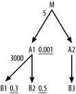
Tip
The one, uncommon case in which joining to the detail table by hash join pays off, at least a little, occurs when the cumulative filter product (the product of the already-reached filter ratios) before the detail join lies in the range where you might prefer a full table scan of the details. This case generally implies either a poorly filtered query that returns more rows than are useful, unless the tables are so small that optimization does not matter, or a rare query with many poor filters combined across different branches under the detail table.
On the other hand, when you join downward to a master table, you
might be joining to a much smaller table, and the cost of reaching the
rows through the primary key might be larger than the cost of reading
the table independently for a hash join. From the statistics in Figure 6-32, you would find
3,000 times as many rows in A1 as
in B1. Even discarding 999 out of
1,000 rows from A1, the database
would join to each row in B1 an
average of three times. Assume that A1 has 3,000,000 rows and B1 has 1,000 rows. After winnowing A1 down to 3,000 rows, using the driving
filter, the database would join to rows in the 1,000-row table
B1 3,000 times. If the database
drove into B1 with B1’s own filter, it would need to read just
300 (0.3 x 1,000) rows, at roughly 1/10th
the cost. Since the query reaches over 20% of the rows in B1, the database would find an even lower
cost by simply performing a full table scan of B1 and filtering the result before doing the
hash join. Therefore, while leaving the rest of the query cost
unchanged, choosing a hash join to B1 would eliminate almost all the cost of
the B1 table reads, compared to the
standard robust plan that reads B1
through nested loops.
So, especially when you see large detail join ratios,
hash joins to master tables can be fastest. How big is the
improvement, though? In the example, the fractional improvement for
this one table was high, over 90%, but the absolute improvement was
quite modest, about 9,000 logical I/Os (6,000 in the two-level-deep
key index and 3,000 on the table), which would take about 150
milliseconds. You would find no physical I/O at all to a table and
index of this size. On the other hand, you would find the query reads
about 2,250 (3,000 x 0.3 x 0.5 x 5) rows from the 15,000,000-row table
M with 3,600 logical I/Os.
Tip
Nested loops drive 450 (3,000 x 0.3 x 0.5) range scans on the
foreign-key index leading to M,
and these range scans require 1,350 (450 x 3) logical I/Os in the
three-level-deep index. 2,250 logical I/Os to the table follow, to
read the 2,250 rows in M. Thus,
the total number of logical I/Os is 3,600 (1,350+2,250).
These 3,600 logical I/Os, especially the 2,250 to the table
itself, will lead to hundreds of physical I/Os for such a large,
hard-to-cache table. At 5-10 milliseconds per physical I/O, the reads
to M could take seconds. This
example is typical of cases in which hash joins perform best; these
cases tend to deliver improvements only in logical I/Os to the
smallest tables, and these improvements tend to be slight compared to
the costs of the rest of the query.
A couple of rough formulae might help you choose the best join method:
| H=C x R |
| L=C x D x F x N |
The variables in these formulas are defined as follows:
- H
The number of logical I/Os necessary to read the master table independently, for purposes of a hash join.
- C
The rowcount of the master table.
- R
The master table’s filter ratio. Assume the database reaches the table independently, through an index range scan on that filter.
- L
The number of logical I/Os to read the master table through nested loops on its primary key.
- D
The detail join ratio for the link that leads up from the master table, which normally tells you how much smaller it is than the detail table above it.
- F
The product of all filter ratios, including the driving filter ratio, reached before this join.
- N
The number of logical I/Os required per row read through the primary-key index.
Since primary keys up to 300 rows normally fit in the root block, N=2 (1 for the index root block and 1 for the table) for C up to 300. N=3 for C between roughly 300 and 90,000. N=4 for C between 90,000 and 27,000,000. Since you will normally drive from the best filter ratio, F<R, even if the plan picks up no additional filters after the driving-table filter.
H is less than L, favoring the hash join for logical I/O costs, when R<D x F x N. F<R when you drive from the node with the best filter ratio. N is small, as shown, since B-trees branch heavily at each level. Therefore, to favor a hash join, either F is close in magnitude to R, or D is large, making this a join to a much smaller master table. This same calculation will sometimes show a logical-I/O savings when joining to a large master table, but use caution here. If the master table is too large to cache easily, physical I/O comes into play and tends to disfavor the hash join in two ways:
Since table rows are much less well cached than index blocks, the hash-join cost advantage (if any) when physical I/O costs dominate mostly compares just the table-row counts, asking whether R<D x F. Since I/O to the index is so much better cached than I/O to the table, costs dominated by physical I/O lose the N factor for index-block reads. Without the N factor, hash joins are less favored.
If C x R is large, the hash join might have to write prehashed rows to disk and read them back, making the hash join much more expensive and potentially leading to out-of-disk errors for disk caching during query execution. This is the robustness risk of foregoing nested loops.
In all, it is difficult to find real queries that yield a hash-join savings over the best robust plan that are worth much bother. Almost the only cases of large savings for hash joins appear when the query starts with a poor driving filter and hits large tables, which almost inevitably means the whole query will usually return an unreasonably large rowset.
However, none of this implies that hash joins are a mistake; cost-based optimizers look for small improvements as well as large, and they are good at finding cases in which hash joins help a bit. While I almost never go out of my way to force a hash join, I usually do not attempt to override the optimizer’s choice when it chooses one for me on a small table, as it often does, as long as the join order and index choices are still good. If in doubt, you can always experiment. First, find the best robust nested-loops plan.
Tip
If you do not start with the best join order, replacing a nested-loops join with a hash join can easily lead to big savings, because then the early tables do not guarantee coming from the best filters (i.e., they do not guarantee F<R). Poorly optimized join orders can execute the join-key lookups an excessive number of times. If you find a query that showed dramatic improvement with a hash join, you should suspect that it had the wrong join order or failed to reach the joined table through the index on the full join key.
Then, replace nested loops to a master table with an optimized single-table access path to the same table and a hash join at the same point in the join order. This change will not affect costs to the other tables, decoupling the choice from the other optimization choices. Use whichever choice is fastest, keeping in mind that you must rerun tests or run tests far apart to avoid a caching bias against the first test.
The earlier example, in Section 6.3.1, of the
problem diagrammed in Figure
6-2 illustrates well a minor performance improvement available
through hash joins. Notice that the detail join ratios above nodes
OT and ODT are in the millions, indicating that
these are joins to a tiny set of rows of the Code_Translations table. Since each set of
eligible rows for the given values of Code_Type is so small, you will require less
logical I/O to read the whole rowset once, probably through an index
on the Code_Type column, then
perform a hash join, rather than go to each row (more than once,
probably) as you need it, though nested loops. Either alternative is
cheap, though, and will make up just a small fraction of the overall
query runtime, since the number of rows the query returns is modest
and the physical index and table blocks of Code_Translations will be fully
cached.
Exercise (See Section A.2 for the solution to the exercise.)
Here’s an exercise that puts it all together with more filters and exceptions in a single query than you are likely to see in your life. Figure 6-33 is a more complex and difficult query diagram than I’ve ever encountered in a real-world tuning problem.
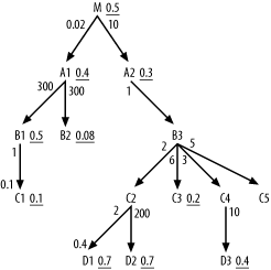
If you can handle this, you can easily handle any query diagram
you will ever find in real life, so give it a shot! (If you don’t get it
right the first time, come back and try again after more practice.) Find
the best join order. Find the best join method for each join, assuming
table A1 has 30,000,000 rows and
assuming a full table scan is preferable for any table on which you will
read at least 5% of the rows. Find the set of primary-key indexes
needed, the set of foreign-key indexes needed, and any other indexes
needed. Find any modifications to the SQL needed to pick up hidden
filters soonest. Make the usual assumptions about referential
integrity.