
Appendix B. The Full Process, End to End
Do not delay, Do not delay: the golden moments fly!
Throughout the book, there are examples that illustrate each step of the process in detail, but I have not yet followed a single example through the entire process. If you like seeing whole processes from end to end and working from those examples, this appendix is for you.
The example in this appendix follows a query that is just complex enough to illustrate the main points that come up repeatedly, while having something wrong that needs fixing. Imagine that the following query were proposed for an application designed to run well on Oracle, DB2, and SQL Server, and you were asked to pass judgement regarding its optimality on those databases and to propose changes to tune it as needed:
SELECT C.Phone_Number, C.Honorific, C.First_Name, C.Last_Name, C.Suffix,
C.Address_ID, A.Address_ID, A.Street_Addr_Line1, A.Street_Addr_Line2,
A.City_Name, A.State_Abbreviation, A.ZIP_Code, OD.Deferred_Ship_Date,
OD.Item_Count, P.Prod_Description, S.Shipment_Date
FROM Orders O, Order_Details OD, Products P, Customers C, Shipments S,
Addresses A
WHERE OD.Order_ID = O.Order_ID
AND O.Customer_ID = C.Customer_ID
AND OD.Product_ID = P.Product_ID
AND OD.Shipment_ID = S.Shipment_ID
AND S.Address_ID = A.Address_ID
AND C.Phone_Number = 6505551212
AND O.Business_Unit_ID = 10
ORDER BY C.Customer_ID, O.Order_ID Desc, S.Shipment_ID, OD.Order_Detail_ID;
Reducing the Query to a Query Diagram
For the first step in the process, create a query diagram. Start with a query skeleton, and then add detail to complete the diagram. The next few subsections walk you through the process of creating the diagram for the example query.
Creating the Query Skeleton
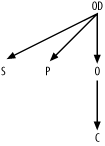
As a starting point, place a random alias in the center of the
diagram under construction. For illustration purposes, I’ll begin with
the node O. Draw arrows downward
from that node to any nodes that join to O through their primary key (named, for all
these tables, by the same name as the table, with the s at the end replaced by _ID). Draw a downward-pointing arrow from
any alias to O for any join that
joins to O on the Orders table’s primary key, Order_ID. The beginning of the query
skeleton should look like Figure
B-1.
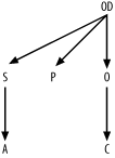
Now, shift focus to OD. Find
joins from that node, and add those links to the join skeleton. The
result is shown in Figure
B-2.
Find undiagramed join conditions. The only one left is S.Address_ID = A.Address_ID, so add a link
for that join to complete the query skeleton, as shown in Figure B-3.
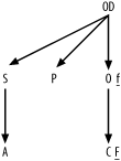
Creating a Simplified Query Diagram
To build the simplified query diagram, find the most
selective filter and identify it with an underlined F next to the filtered node. The condition
on the customer’s phone number is almost certainly the most selective
filter. Add a small underlined f
for the only other filter, the much less selective condition on
Business_Unit_ID for Orders. The result, shown in Figure B-4, is the simplified
query diagram.
Creating a Full Query Diagram
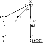
The simplified query diagram is sufficient to tune this particular query. However, for purposes of illustration, I will show the creation of a full query diagram, with all the details. Use the following queries to gather statistics necessary for a full query diagram. The results I’m using for this example are shown following each query. As an exercise, you might wish to work out the filter and join ratios for yourself.
Q1: SELECT SUM(COUNT(Phone_Number)*COUNT(Phone_Number))/(SUM(COUNT(Phone_Number))*SUM(COUNT(*))) A1FROM CustomersGROUP BY Phone_Number;A1: 0.000003Q2: SELECT COUNT(*) A2 FROM Customers;A2: 500,000Q3: SELECT SUM(COUNT(Business_Unit_ID)*COUNT(Business_Unit_ID))/(SUM(COUNT(Business_Unit_ID))*SUM(COUNT(*))) A3FROM OrdersGROUP BY Business_Unit_ID;A3: 0.2Q4: SELECT COUNT(*) A4 FROM Orders;A4: 400,000Q5: SELECT COUNT(*) A5FROM Orders O, Customers CWHERE O.Customer_ID = C.Customer_ID;A5: 400,000Q6: SELECT COUNT(*) A6 FROM Order_Details;A6: 1,200,000Q7: SELECT COUNT(*) A7FROM Orders O, Order_Details ODWHERE OD.Order_ID = O.Order_ID;A7: 1,2000,000Q8: SELECT COUNT(*) A8 FROM Shipments;A8: 540,000Q9: SELECT COUNT(*) A9FROM Shipments S, Order_Details ODWHERE OD.Shipment_ID = S.Shipment_ID;A9: 1,080,000Q10: SELECT COUNT(*) A10 FROM Products;A10: 12,000Q11: SELECT COUNT(*) A11FROM Products P, Order_Details ODWHERE OD.Product_ID = P.Product_ID;A11: 1,200,000Q12: SELECT COUNT(*) A12 FROM Addresses;A12: 135,000Q13: SELECT COUNT(*) A13FROM Addresses A, Shipments SWHERE S.Address_ID = A.Address_ID;A13: 540,000
Tip
I downsized the tables in this example so that I could provide practical data-generation scripts to test the execution plans that cost-based optimizers will generate for these tables. If you want to follow along with the example, you can download these scripts from the O’Reilly catalog page for this book: http://www.oreilly.com/catalog/sqltuning/. (However, I cannot guarantee identical results, since results depend on your database version number, parameters set by your DBA, and the data.) The larger tables in this example would likely be around 10 times bigger in a production environment.
Beginning with filter ratios, get the weighted-average
filter ratio for the condition on Customers Phone_Number directly from A1, which is the result from query Q1 (0.000003). Find the filter ratio on
Orders the same way, from Q3, which returns the result of 0.2 for
A3.
Since no other alias has any filters, the filter ratios on the other four are 1.0, which you imply by just leaving filter ratios off the query diagram for the other nodes.
For each join, find the detail join ratio, to place
alongside the upper end of each join arrow, by dividing the count on
the join of the two tables by the count on the lower table (the master
table of that master-detail relationship). The ratios for the upper
ends of the joins from OD to
S, O, and P
are 2 (A9/A8), 3 (A7/A4),
and 100 (A11/A10), respectively. The ratio for the upper
end of the join from S to A is 4 (A13/A12).
The ratio for the upper ends of the join from O to C is
0.8 (A5/A2).
Find the master join ratios, to place alongside the
lower end of each join arrow, by dividing the count on the join of the
two tables by the count on each upper table (the detail table of a
master-detail relationship). The ratio for the lower end of the join
from OD to S is 0.9 (A9/A6).
All the other master join ratios turn out to be 1.0, so leave these
off the diagram.
Add filter ratios and join ratios to the query skeleton (see Figure B-3) to create the full query diagram, as shown in Figure B-5.
Solving the Query Diagram
After you’ve reduced the detail-filled query to an abstract join diagram, you are 80% of the way to finding the best execution plan, just as math word problems usually become trivial once you convert them to symbolic form. However, you still must solve the symbolic problem. Using the methods of Chapter 6, solve the problem abstracted in Figure B-5:
Choose the best driving table. By far, the best (closest to 0) filter ratio is on
C, so chooseCas the driving table.From
C, you find no downward joins, so you choose the only upward join, toO, placingOsecond in the join order.
Tip
Even if there were downward joins available from C, you would still consider joining to
O early, since the detail join
ratio to O is less than 1.0 and
since O has a good filter
itself.
From
O, you find no unused downward joins, so you choose the only upward join, toOD, placingODthird in the join order.From
OD, you find two unused downward joins, toSand toP. There are no more simple filters on the remaining nodes, but there is a hidden join filter in the join toS, since the master join ratio on that join is less than 1.0. Therefore, join toSnext, placingSfourth in the join order.
Tip
If there were a filter on node P, you would make the implicit filter
OD.Shipment_ID IS NOT NULL (which
is implied by the master join ratio to S being less than 1.0) explicit, so you
could pick up that filter early without joining to S and reach the filter on P after getting the benefit of that NOT NULL filter, without paying the added
price of joining to S before
P.
The remaining nodes,
AandP, are both unfiltered, are reachable directly with joins from tables already reached, and have master join ratios equal to 1.0, so it makes no difference which order you join to these last two nodes. Just to make the rest of the problem concrete, arbitrarily chooseAas the fifth in the join order and then choosePas the last. This leads you to the optimum join order of(C, O, OD, S, A, P).Given the join order, specify the full execution plan, following the rules for robust execution plans, in the optimum join order:
Drive to the first table,
Customers, on an index on the filter column,Phone_Number, with a query modified if necessary to make that index accessible and fully useful.With nested loops, join to
Orderson an index on the foreign keyCustomer_ID.With nested loops, join to
Order_Detailson an index on the foreign keyOrder_ID.With nested loops, join to
Shipmentson its primary-key index onShipment_ID.With nested loops, join to
Addresseson its primary-key index onAddress_ID.With nested loops, join to
Productson its primary-key index onProduct_ID.
This completes the second step in the tuning process: finding the execution plan that you want. Next, you need to see which execution plan you actually get, on all three databases, since this example illustrates SQL that is designed to run on any of the three.
Checking the Execution Plans
For this exercise, imagine that the base development is performed on Oracle, with later testing to check that the same SQL functions correctly and performs well on DB2 and SQL Server. You learned of this SQL because it performed more slowly than expected on Oracle, so you already suspect it leads to a poor execution plan on at least that database. You will need to check execution plans on the other databases, which have not yet been tested.
Getting the Oracle Execution Plan
Place the SQL in a file named tmp.sql and run the script ex.sql, as described in Chapter 3. The result is as follows:
PLAN
--------------------------------------------------------------------------------
SELECT STATEMENT
  SORT ORDER BY
    NESTED LOOPS
      NESTED LOOPS
        NESTED LOOPS
          NESTED LOOPS
            NESTED LOOPS
              TABLE ACCESS FULL 4*CUSTOMERS
              TABLE ACCESS BY INDEX ROWID 1*ORDERS
                INDEX RANGE SCAN ORDER_CUSTOMER_ID
            TABLE ACCESS BY INDEX ROWID 2*ORDER_DETAILS
              INDEX RANGE SCAN ORDER_DETAIL_ORDER_ID
          TABLE ACCESS BY INDEX ROWID 5*SHIPMENTS
            INDEX UNIQUE SCAN SHIPMENT_PKEY
        TABLE ACCESS BY INDEX ROWID 6*ADDRESSES
          INDEX UNIQUE SCAN ADDRESS_PKEY
      TABLE ACCESS BY INDEX ROWID 3*PRODUCTS
        INDEX UNIQUE SCAN PRODUCT_PKEY
You notice that your database is set up to use the rule-based optimizer, so you switch to cost-based optimization, check that you have statistics on the tables and indexes, and check the plan again, finding a new result:
PLAN
--------------------------------------------------------------------------------
SELECT STATEMENT
  SORT ORDER BY
    HASH JOIN
      TABLE ACCESS FULL 3*PRODUCTS
      HASH JOIN
        HASH JOIN
          HASH JOIN
            HASH JOIN
              TABLE ACCESS FULL 4*CUSTOMERS
              TABLE ACCESS FULL 1*ORDERS
            TABLE ACCESS FULL 2*ORDER_DETAILS
          TABLE ACCESS FULL 5*SHIPMENTS
        TABLE ACCESS FULL 6*ADDRESSES
Neither execution plan is close to the optimum plan. Instead, both the rule-based and the cost-based optimization plans drive from full table scans of large tables. The database ought to reach the driving table on a highly selective index, so you know that an improvement is certainly both necessary and possible.
Getting the DB2 Execution Plan
Place the SQL in tmp.sql and run the following command according to the process described in Chapter 3:
cat head.sql tmp.sql tail.sql | db2 +c +p -t
The result is an error; DB2 complains that it sees inconsistent
column types in the condition on Phone_Number. You discover that the Phone_Number column is of the VARCHAR type, which is incompatible with the
number type of the constant 6505551212.
Unlike Oracle, DB2 does not implicitly convert character-type
columns to numbers when SQL compares inconsistent datatypes. This is
just as well, in this case, since such a conversion might deactivate
an index on Phone_Number, if there
is one. You might even suspect, already, that this is precisely what
has caused poor performance in the Oracle baseline development
environment.
You fix the problem in the most obvious way, placing quotes around the phone number constant to make it a character type:
SELECT C.Phone_Number, C.Honorific, C.First_Name, C.Last_Name, C.Suffix,
C.Address_ID, A.Address_ID, A.Street_Addr_Line1, A.Street_Addr_Line2,
A.City_Name, A.State_Abbreviation, A.ZIP_Code, OD.Deferred_Ship_Date,
OD.Item_Count, P.Prod_Description, S.Shipment_Date
FROM Orders O, Order_Details OD, Products P, Customers C, Shipments S,
Addresses A
WHERE OD.Order_ID = O.Order_ID
AND O.Customer_ID = C.Customer_ID
AND OD.Product_ID = P.Product_ID
AND OD.Shipment_ID = S.Shipment_ID
AND S.Address_ID = A.Address_ID
AND C.Phone_Number = '6505551212'
AND O.Business_Unit_ID = 10
ORDER BY C.Customer_ID, O.Order_ID Desc, S.Shipment_ID, OD.Order_Detail_ID;
Placing this new version of the SQL in tmp.sql, you again attempt to get the execution plan:
$cat head.sql tmp.sql tail.sql | db2 +c +p -t
DB20000I  The SQL command completed successfully.
DB20000I  The SQL command completed successfully.

OPERATOR_ID TARGET_ID OPERATOR_TYPE OBJECT_NAME        COST
----------- --------- ------------- ------------------ -----------
          1         - RETURN        -                          260
          2         1 NLJOIN        -                          260
          3         2 NLJOIN        -                          235
          4         3 NLJOIN        -                          210
          5         4 TBSCAN        -                          185
          6         5 SORT          -                          185
          7         6 NLJOIN        -                          185
          8         7 NLJOIN        -                          135
          9         8 FETCH         CUSTOMERS                   75
         10         9 IXSCAN        CUST_PH_NUMBER              50
         11         8 FETCH         ORDERS                      70
         12        11 IXSCAN        ORDER_CUST_ID               50
         13         7 FETCH         ORDER_DETAILS               75
         14        13 IXSCAN        ORDER_DTL_ORD_ID            50
         15         4 FETCH         PRODUCTS                    50
         16        15 IXSCAN        PRODUCT_PKEY                25
         17         3 FETCH         SHIPMENTS                   75
         18        17 IXSCAN        SHIPMENT_PKEY               50
         19         2 FETCH         ADDRESSES                   75
         20        19 IXSCAN        ADDRESS_PKEY                50

  20 record(s) selected.

DB20000I  The SQL command completed successfully.
$
That’s more like it, just the execution plan you chose when you
analyzed the SQL top-down, except for the minor issue of reaching
Products before Shipments, which will have virtually no
effect on the runtime. Since the type inconsistency involving Phone_Number might require correcting on SQL
Server and Oracle, you need to try this modified version immediately
on the other databases.
Getting the SQL Server Execution Plan
Suspecting that you already have the solution to slow
performance for this query, you fire up SQL Server’s Query Analyzer and use set showplan_text on to see a concise view
of the execution plan of the statement modified with C.Phone_Number = '6505551212' to correct the type
inconsistency. A click on the Query Analyzer’s Execute-Query button
results in the following output:
StmtText
-------------------------------------------------------------------------------
  |--Bookmark Lookup(...(...[Products] AS [P]))
       |--Nested Loops(Inner Join)
            |--Bookmark Lookup(...(...[Addresses] AS [A]))
            |    |--Nested Loops(Inner Join)
            |         |--Sort(ORDER BY:([O].[Customer_ID] ASC, [O].[Order_ID] DESC,(wrapped line) [OD].[Shipment_ID] ASC, [OD].[Order_Detail_ID] ASC))
            |         |    |--Bookmark Lookup(...(...[Shipments] AS [S]))
            |         |         |--Nested Loops(Inner Join)
            |         |              |--Bookmark Lookup(...(...[Order_Details] AS
[OD]))
            |         |              |    |--Nested Loops(Inner Join)
            |         |              |         |--Filter(WHERE:([O].[Business_Unit_
ID]=10))
            |         |              |         |    |--Bookmark Lookup(...(...
[Orders] AS [O]))
            |         |              |         |         |--Nested Loops(Inner Join)
            |         |              |         |              |--Bookmark Lookup(...
(...
(wrapped line) [Customers] AS [C]))
            |         |              |         |              |    |--Index Seek(...
(...
(wrapped line) [Customers].[Customer_Phone_Number]
(wrapped line) AS [C]), SEEK:([C].[Phone_Number]='6505551212') ORDERED)
            |         |              |         |              |--Index Seek(...(...
(wrapped line) [Orders].[Order_Customer_ID] AS [O]),
(wrapped line) SEEK:([O].[Customer_ID]=[C].[Customer_ID]) ORDERED)
            |         |              |         |--Index Seek(...(...
(wrapped line) [Order_Details].[Order_Detail_Order_ID]
(wrapped line) AS [OD]), SEEK:([OD].[Order_ID]=[O].[Order_ID]) ORDERED)
            |         |              |--Index Seek(...(...[Shipments].[Shipment_PKey]
(wrapped line) AS [S]), SEEK:([S].[Shipment_ID]=[OD].[Shipment_ID]) ORDERED)
            |         |--Index Seek(...(...[Addresses].[Address_PKey]
(wrapped line) AS [A]), SEEK:([A].[Address_ID]=[S].[Address_ID]) ORDERED)
            |--Index Seek(...(...[Products].[Product_PKey]
(wrapped line) AS [P]), SEEK:([P].[Product_ID]=[OD].[Product_ID]) ORDERED)

(19 row(s) affected)
Good news! The corrected SQL leads to exactly the optimum plan here. Just out of curiosity, you check the execution plan for the original SQL, and you find the same result! Evidently, SQL Server is doing the data conversion on the constant, avoiding disabling the index.
Altering the Database to Enable the Best Plan
The earlier results on DB2 and SQL Server have already
demonstrated that the database design has the necessary indexes to
enable the execution plan that you need, unless the Oracle database is
missing indexes that you have on the other databases. Therefore, you
could skip this step. However, if you did not already know that they
existed, you would check for indexes on Customers(Phone_Number), Orders(Customer_ID), and Order_Details(Order_ID) using the methods of
Chapter 3. You can generally take
for granted that the primary-key indexes that you need already exist.
Look for missing primary-key indexes only when more likely reasons for
an incorrect execution plan do not solve the problem and lead you to
check for unusual sources of trouble.
Altering the SQL to Enable the Best Plan
You already suspect that the solution to getting a good
plan on Oracle is to eliminate the type inconsistency on that platform.
After all, the other databases avoided the type conversion on the
indexed column and delivered a good plan. Therefore, immediately try the
query again on Oracle, but with the corrected comparison C.Phone_Number = '6505551212' to avoid the
implicit datatype conversion. Use the original setting for rule-based
optimization to check the execution plan:
PLAN
--------------------------------------------------------------------------------
SELECT STATEMENT
  SORT ORDER BY
    NESTED LOOPS
      NESTED LOOPS
        NESTED LOOPS
          NESTED LOOPS
            NESTED LOOPS
              TABLE ACCESS BY INDEX ROWID 4*CUSTOMERS
                INDEX RANGE SCAN CUSTOMER_PHONE_NUMBER
              TABLE ACCESS BY INDEX ROWID 1*ORDERS
                INDEX RANGE SCAN ORDER_CUSTOMER_ID
            TABLE ACCESS BY INDEX ROWID 2*ORDER_DETAILS
              INDEX RANGE SCAN ORDER_DETAIL_ORDER_ID
          TABLE ACCESS BY INDEX ROWID 5*SHIPMENTS
            INDEX UNIQUE SCAN SHIPMENT_PKEY
        TABLE ACCESS BY INDEX ROWID 3*PRODUCTS
          INDEX UNIQUE SCAN PRODUCT_PKEY
      TABLE ACCESS BY INDEX ROWID 6*ADDRESSES
        INDEX UNIQUE SCAN ADDRESS_PKEY
This is precisely the execution plan you want. Suspecting that the application will soon switch to cost-based optimization, you check the cost-based execution plan, and it turns out to be the same.
Both Oracle optimizers now return the optimal plan, so you should
be done! To verify this, you run the SQL with the sqlplus option set
timing on and find that Oracle returns the result in just 40
milliseconds, compared to the earlier performance of 2.4 seconds for the
original rule-based execution plan and 8.7 seconds for the original
cost-based execution plan
Altering the Application
As is most commonly the case, the only change the application needs, in this example, is the slight change to the SQL itself. This is always the most favorable result, since such SQL-only changes have the lowest risk and are the easiest to make. This query will return just a few rows, since the best filter, alone, is so selective. If the query returned excessively many rows, or if the query ran excessively often just to perform a single application task, you would explore changes to the application to narrow the query or to run it less often.
Putting the Example in Perspective
Most queries are just this easy to tune, once you master the method this book describes. Usually, a missing index or some trivial problem in the SQL is the only thing obstructing the optimizer from delivering the optimum execution plan you choose, or a plan so close to optimum as not to matter. You rarely need the elaborate special techniques covered at the end of Chapter 6 and throughout Chapter 7.
The primary value of the method is that it leads you quickly to a single answer you can be completely confident in, without any nagging worries that long trial and error might just lead you to something better. When the method leads you to a super-fast query, you find little argument. When the method leads to a slower result than you’d like (usually for a query that returns thousands of rows), you need to know that the slower result really is the best you can do without stepping outside the SQL-tuning box. The outside-the-box solutions for these slower queries tend to be inconvenient. It’s invaluable to know with complete confidence when these inconvenient solutions are truly necessary. You need to justify this confidence without endless, futile attempts to tune the original SQL by trial and error, and with solid arguments to make your case for more difficult solutions when needed.