
Appendix A. Exercise Solutions
When I rest, I rust [Rast ich, so rost ich].
This appendix contains solutions to the exercises in Chapter 5 through Chapter 7.
Chapter 5 Exercise Solutions
Following are the solutions to the exercises in Section 5.5.
Exercise 1
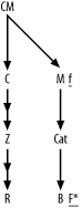
Figure A-1 shows the solution to Exercise 1.
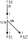
The subtlest aspect of this exercise is that you need to notice
that you do not need queries (other than the total table rowcounts) to
find the filter ratios for the R
and D nodes. From the exact matches
on uniquely indexed names for each of these, a single match for
R and an IN list for D, you can deduce the ratios. You just need
to calculate 1/R and 2/D, where D and R are the respective rowcounts of those
tables, to find their filter ratios. Did you remember to add the
* to the filter ratio on R to indicate that it turns out to be a
unique condition? (This turns out to be important for optimizing some
queries!) You would add an asterisk for the condition on D, as well, if the match were with a single
name instead of a list of names.
The other trick to notice is that, by the assumption of never-null foreign keys with perfect referential integrity, the rowcounts of the joins would simply equal the rowcounts of the detail tables. Therefore, the detail join ratios are simply d/m, where d is the rowcount of the upper detail table and m is the rowcount of the lower master table. The master join ratios under the same assumptions are exactly 1.0, and you simply leave them off.
Exercise 2
Figure A-2 shows the solution to Exercise 2.
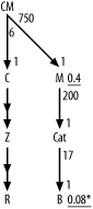
In this problem, you need the same shortcuts as for Exercise 1,
for join ratios and for the filter ratio to B. Did you remember to add the * for the unique filter on B? Did you remember to indicate the
direction of the outer joins to Z
and R with the midpoint arrows on
those join links?
Exercise 3
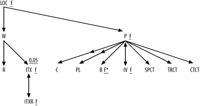
Figure A-3 shows the solution to Exercise 3.
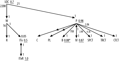
In this problem, you need the same tricks as for Exercise 1, for
join ratios and for the filter ratio to B. Did you remember to add the * for the unique filter on B? Did you remember to indicate the
direction of the outer joins to C
and PL with the midpoint arrows on
those join links?
The joins to ITxR and
IV from ITx and P, respectively, are special one-to-one
joins that you indicate with arrows on both ends of the join links.
The filter ratios on both ends of these one-to-one joins are exactly
1.0. These are a special class of detail table that frequently comes
up in real-world applications: time-dependent details that have one
row per master row corresponding to any given effective date. For
example, even though you might have multiple inventory tax rates for a
given taxing entity, only one of those rates will be in effect at any
given moment, so the date ranges defined by Effective_Start_Date and Effective_End_Date will be nonoverlapping.
Even though the combination of ID and date-range condition do not
constitute equality conditions on a full unique key, the underlying
valid data will guarantee that the join is unique when it includes the
date-range conditions.
Since you count the date range defined by Effective_Start_Date and Effective_End_Date as part of the join, do
not count it as a filter, and consider only the subtable that meets
the date-range condition as effective for the query diagram. Thus, you
find P and IV to have identical effective rowcounts of
8,500, and you find identical rowcounts of 4 for ITx and ITxR. This confirms the one-to-one nature of
these joins and the join ratios of 1.0 on each end of the
links.
As for the example in Figure 5-4, you should use only
subtable rowcounts for the joins to SPCT, TRCT, and CTCT, because Code_Translations is one of those
apples-and-oranges tables that join only a specific subtable at a
time.
Exercise 4
Figure A-4 shows the solution to Exercise 4, the fully simplified solution to Exercise 1.
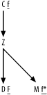
Since this problem involves only large detail join ratios and
master join ratios equal to 1.0, you just add a capital F to the most highly filtered node and add
a lowercase f to the other
filtered nodes, with an asterisk for the unique filter on node
R. (Did you remember the
asterisk?)
Exercise 5
Figure A-5 shows the solution to Exercise 5, the fully simplified solution to Exercise 2.
Since this problem involves only large detail join ratios, and
master join ratios equal to 1.0, you just add a capital F to the most highly filtered node and add
a lowercase f to the other
filtered node, with an asterisk for the unique filter on node B. (Did you remember the asterisk?)
Exercise 6
Figure A-6 shows the solution to Exercise 6, the fully simplified solution to Exercise 3.
Since this problem involves only large detail join ratios, you
can leave those out. However, note that it does include one master
join ratio well under 1.0, in the join down into ITx, so you leave that one in. Otherwise,
you just add a capital F to the
most highly filtered node and add a lowercase f to the other filtered nodes, with an
asterisk for the unique filter on node B. (Did you remember the
asterisk?)
Chapter 6 Exercise Solution
Section 6.7 included only one, outrageously complicated problem. This section details the step-by-step solution to that problem.
Figure A-7 shows how to adjust effective filters to take account of join factors less than 1.0, which occur in three places in Figure 6-33.
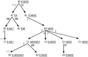
You adjust effective filters immediately on either side of the
master join ratios, since you can migrate those filters upward with
explicit IS NOT NULL conditions on
the foreign keys. This adjusts filters on B1, C1,
C2, and D1, and you cross out the master join ratios
to show that you took them into account. Note the detail join ratio of
0.02 between M and A1 for even bigger adjustments on every filter
from M down through the A2 branch.
Tip
If there were other branches, you would adjust them as well.
Only the A1 branch, attached
through that filtering join, does not see the adjustment.
Note that you adjust the effective join ratio for C2 and D1
twice, since two filtering joins affect these. Working through the
numbers, you find the best effective filter, 0.004 (0.2 x 0.02), lies on
C3, so that is the driving
table.
After choosing the driving table, you need a whole new set of
adjustments to take account of the two low master join ratios before
choosing the rest of the join order. Note that you no longer need to
take account of the detail join ratio, since the database is coming from
the side of the join that does not discard rows through the join. This
happens whenever you choose a driving table with an effective filter
adjusted by the detail join ratio. In a sense, you burn the filter at
the beginning, coming from smaller tables that point to only a subset of
the master table (A1 in this case) on
the other side of that join.
It is best to get the benefit of the hidden join filters that
point to C1 and D1 as early in the join order as possible.
Therefore, make explicit the is-not-null filters on the foreign keys (in
B1 and C2) that point to these filtering joins, as
shown in Figure A-8. By
making these filters explicit (and assuming referential integrity), you
no longer see filtering in the joins themselves, so you cross out those
join ratios.
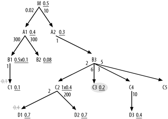
From C3, you can join only to
B3, so it is next in the join order.
From these two, you can join to C2,
C4, C5 (below), or A2 (above). Normally, you would consider
joining only next to the tables below, but notice that the detail join
ratio to A2 is 1.0, so it is eligible
early and, in fact, it turns out to have the best effective filter of
the choices, so you join to it next. This adds M to the list of nodes now in reach, but the
detail join ratio to M is high, so
postpone that join as long as possible. The only eligible node below
with a filter is now C2, thanks to
the now-explicit not-null condition on the foreign key that points to
D1, so join to C2 next. The join order, so far, is (C3, B3, A2, C2).
The join to C2 adds D1 and D2
to the list of eligible nodes downward from the joined tables so far,
and these are the only eligible tables in that direction with filters,
so choose one of them next. The filter ratios are identical, so look at
other considerations to break the tie and note that D2 must be smaller, since the detail join
ratio above it is much larger. Therefore, following the
smaller-table-first tiebreaker, join to D2 before D1. The join order, so far, is (C3, B3, A2, C2, D2, D1).
Between C4 and C5, you also have a tie on filter ratios
(unshown) equal to 1.0, but you break the tie with the filter-proximity
rule that favors C4 for the path it
provides to the filter on D3. After
reaching C4, go to D3 for that filter and finally join to the
unfiltered C5. The join order, so
far, is (C3, B3, A2, C2, D2, D1, C4, D3,
C5).
From here, there is no choice in the next node, the upward join to
M. After reaching M, there is again no choice; A1 is the only node attached. At this point,
you could join to either B1 or
B2. Their filter ratios are nearly a
tie for purposes of later joins, but their detail join ratios are the
same, so they should be the same size, leaving table size out of the
picture. You can also leave proximity out of the picture, because the
filter on C1 is no better than the
filter on B1. With no reason to
override going to the best filter, on B1, you choose to join to it next. This leaves
the join order, so far, of (C3, B3, A2,
C2, D2, D1, C4, D3, C5, M, A1,
B1). The only two nodes left, B2 and C1,
are both eligible now. B2 has the
better filter, and the combination of master join ratio and detail join
ratio to C1 shows it to be 1/10th the
size of B1. B1, in turn, was the same size as B2, so B2
and C1 are different in size by a
factor of 10, probably enough for the smaller-table-first tiebreaker
rule to favor C1 in the near-tie
between B2 and C1. Therefore, go with C1 first, leaving the complete join order of
(C3, B3, A2,
      C2
, D2, D1, C4, D3, C5, M, A1, B1, C1, B2).
Tip
These last few joins actually will affect the query cost very little, since the query will be down to a few rows by this point.
To reach the root table from C3, for a robust nested-loops plan, the
database needs foreign-key indexes (from M to A2,
from A2 to B3, and from B3 to C3)
on M, A2, and B3.
You probably need no index at all on C3, since the 20% filter on that table is not
selective enough to make an index outperform a full table scan. (This is
probably a small table, based on the join factors.) All other tables
require indexes on their primary keys to enable a robust plan.
To make the hidden join filters to C1 and D1
explicit and apply them earlier in the plan, add the conditions C2.FkeyToD1 IS NOT NULL AND B1.FkeyToC1 IS NOT
NULL to the query.
Now, relax the robust-plan requirement, and work out which joins
should be hash joins and which access path should be used for the
hash-joined tables. Recall that table A1 has 30,000,000 rows. From the detail join
ratios, B1 and B2 have 1/300th as
many rows: 100,000 each. From the combination of master join ratio and
detail join ratio, C1 has
1/10th as many rows as B1: 10,000. Going up from A1 to M,
M has far fewer (0.02 times as many)
rows as A1: 600,000. Coming down from
M, using detail join ratios,
calculate 60,000 for A2 and B3, 30,000 for C2, 10,000 for C3, 20,000 for C4, and 12,000 for C5. Using both master and detail join ratios
from C2 to D1, calculate 6,000 (30,000 x 0.4/2) rows for
D1. From detail join ratios, find 150
rows in D2 and 2,000 rows in D3.
Any part of the plan that reads more rows from a table than the database would read using the filter on that table tends to favor accessing that table through the filter index and using a hash join at the same point in the original execution plan. Any part of the plan that reads at least 5% of the rows in a table tends to favor a full table scan of that table with a hash join. When both sorts of hash-join access are favored over nested loops (i.e., for a hash join with an indexed read of the filter or with a full table scan), favor the full table scan if the filter matches at least 5% of the table.
Tip
As discussed in Chapter 2, the actual cutoff for indexed access can be anywhere between 0.5% and 20%, but this exercise stated 5% as the assumed cutoff, to make the problem concrete.
In summary, Table A-1 shows the table sizes and full-table-scan cutoffs, arranged in join order.
Table | Rowcount | Full-table-scan cutoff |
| 10,000 | 500 |
| 60,000 | 3,000 |
| 60,000 | 3,000 |
| 30,000 | 1,500 |
| 150 | 8 |
| 6,000 | 300 |
| 20,000 | 1,000 |
| 2,000 | 100 |
| 12,000 | 600 |
| 600,000 | 30,000 |
| 30,000,000 | 1,500,000 |
| 100,000 | 5,000 |
| 10,000 | 500 |
| 100,000 | 5,000 |
Now, working out the rowcounts at each stage of the query, you
find that, after the full table scan to C3, the filter on C3 drops the rowcount to 2,000 rows. Joining
upward with nested loops to B1
touches 12,000 rows of that table, since the detail join ratio is 6.
B3 has no filter, so following the
one-to-one (on average) join to A2
also reaches 12,000 rows, after which the filter on A2 leaves 30% (3,600 rows) for the next join
to C2. With an implied master join
ratio of 1.0, nested loops would touch 3,600 rows of C2. The filters on C2 (including the now-explicit is-not-null
filter on the foreign key to D1)
reduce that rowcount to 1,440 before the join to D2. Nested loops to D2 read 1,440 rows of that table, after which
the filter leaves 1,008 rows. Nested loops to D1 read 1,008 rows of that table (since by
this point all rows have nonnull foreign keys that point to D1), after which the filter leaves 706 rows
(rounding, as I will for the rest of the calculation).
Nested loops to C4 read 706
rows of that table, which are unfiltered, leaving 706. Nested loops to
D3 read 706 rows of that table, after
which the filter leaves 282. Nested loops to C5 read 282 rows of that table, which are
unfiltered, leaving 282. With the detail join ratio of 10, the join
upward into M reaches 2,820 rows of
that table, after which the filter leaves 1,410. With the implied master
join ratio of 1.0, nested loops reach 1,410 rows of the biggest table,
A1, after which the filter leaves
564. Nested loops to B1 read 564 rows
of that table, after which the filters (including the now-explicit
foreign-key-is-not-null condition on the key on B1 that points to C1) leave 28. Nested loops to C1 read 28 rows of that table (since by this
point all rows have nonnull foreign keys that point to C1), after which the filter leaves 3. Nested
loops to B2 read 3 rows of that
table, after which the final filter leaves 0 or 1 row in the final
result.
If you compare these counts of rows reached by nested loops with the full-table-scan cutoffs, you see that hash joins to full table scans reduce cost for several of the tables. Since none of the filters in this query were selective enough to prefer single-table indexed access to full table scans (by the assumed 5% cutoff), you would choose hash joins to rowsets read by full table scans, when you choose hash joins at all. This example shows an unusually favorable case for hash joins. More common examples, with queries of large tables that have at least one selective filter, show fractionally much smaller improvements for hash joins to the smallest tables only.
Table A-2 shows the rowcounts calculated for the best robust plan, alongside the cutoff rowcounts that would result in a hash join to a full table scan being faster. The rightmost column, labeled Method/Join, shows the optimum table access and join methods that result for each table in the leftmost column.
Table | Rowcount | Full-table-scan cutoff | Robust-plan rows reached | Method/Join |
| 10,000 | 500 | 2,000 | Full scan/Driving |
| 60,000 | 3,000 | 12,000 | Full scan/Hash |
| 60,000 | 3,000 | 12,000 | Full scan/Hash |
| 30,000 | 1,500 | 3,600 | Full scan/Hash |
| 150 | 8 | 1,440 | Full scan/Hash |
| 6,000 | 300 | 1,008 | Full scan/Hash |
| 20,000 | 1,000 | 706 | Index/Nested loop |
| 2,000 | 100 | 706 | Full scan/Hash |
| 12,000 | 600 | 282 | Index/Nested loop |
| 600,000 | 30,000 | 2,820 | Index/Nested loop |
| 30,000,000 | 1,500,000 | 1,410 | Index/Nested loop |
| 100,000 | 5,000 | 564 | Index/Nested loop |
| 10,000 | 500 | 28 | Index/Nested loop |
| 100,000 | 5,000 | 3 | Index/Nested loop |
Note that replacing nested-loops joins with hash joins as shown
eliminates the need (for this query, at least) for the foreign-key
indexes on B3 and A2 and the primary-key indexes on C2, D2,
D1, and D3.
Chapter 7 Exercise Solution
Section 7.5 included only one problem, which was deliberately very complex to exercise most of the subquery rules. This section details the step-by-step solution to that problem. Figure A-9 shows the missing ratios for the three semi-joins and the anti-join.
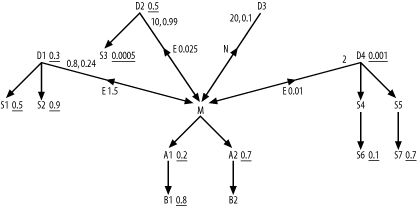
I’ll begin by reviewing the calculation of the missing ratios
shown in Figure A-9. To
find the correlation preference ratio for the semi-join to D1, follow the rules stated in Chapter 7, in Section 7.2.1.1. In Step 1,
you find that the detail join ratio for D1 from Figure 7-36 is D=0.8. This is an uncommon case of a
many-to-one join that averages less than one detail per master row.
Assume M=1, the usual master join
ratio when it is not explicitly shown on the diagram. The best filter
ratio among the nodes of this subquery (D1, S1, and
S2) is 0.3 on D1, so S=0.3. The best filter ratio among the nodes
of the outer query (M, A1, A2,
B1, and B2) is 0.2 for A1, so R=0.2. For Step 2 of the rules, find
D x S=0.24 and M x R=0.2, so D x
S>M x
R. Therefore, proceed to Step 3. You find S>R,
so you set the correlation preference ratio to S/R=1.5,
next to the semi-join indicator E
from M to D1.
To find the correlation preference ratio for the semi-join to
D2, repeat the process. In Step 1,
you find the detail join ratio from Figure 7-36 (D=10). Assume M=1, the usual master join ratio when it is
not explicitly shown on the diagram. The best filter ratio between
D2 and S3 is 0.0005 on S3, so S=0.0005. The best filter ratio among the
nodes of the outer query, as before, is R=0.2. For Step 2 of the rules, find
D x S=0.005 and M x R=0.2, so D x S<M x
R. Therefore, Step 2 completes the
calculation, and you set the correlation preference ratio to (D x S)/(M x
R)=0.025, next to the semi-join
indicator E from M to D2.
To find the correlation preference ratio for the semi-join to
D4, repeat the process. In Step 1,
you find that the detail join ratio from Figure 7-36 is D=2. Assume M=1, the usual master join ratio when it is
not explicitly shown on the diagram. The best filter ratio among
D4, S4, S5,
S6, and S7 is 0.001 on D4, so S=0.001. The best filter ratio among the
nodes of the outer query, as before, is R=0.2. For Step 2 of the rules, find
D x S=0.002 and M x R=0.2, so D x S<M x
R. Therefore, Step 2 completes the
calculation, and you set the correlation preference ratio to (D x S)/(M x
R)=0.01, next to the semi-join
indicator E from M to D4.
Now, shift to the next set of rules, to find the subquery adjusted
filter ratios. Step 1 dictates that you do not need a subquery adjusted
filter ratio for D4, because its
correlation preference ratio is both less than 1.0 and less than any
other correlation preference ratio. Proceed to Step 2 for both D1 (which has a correlation preference ratio
greater than 1.0) and D2 (which has a
correlation preference ratio greater than D4’s correlation preference ratio). The
subqueries under both D1 and D2 have filters, so proceed to Step 3 for
both. For D1, find D=0.8 and s=0.3, the filter ratio on D1 itself. At Step 4, note that D<1, so you set the subquery adjusted
filter ratio equal to s x D=0.24, placed next to the 0.8 on the upper
end of the semi-join link to D1.
At Step 3 for D2, find
D=10 and s=0.5, the filter ratio on D2 itself. At Step 4, note that D>1, so proceed to Step 5. Note that
s x D=5, which is greater than 1.0, so proceed to
Step 6. Set the subquery adjusted filter ratio equal to 0.99, placed
next to the 10 on the upper end of the semi-join link to D2.
The only missing ratio now is the subquery adjusted filter ratio
for the anti-join to D3. Following
the rules for anti-joins, for Step 1, find t=5 and q=50 from the problem statement. In Step 2,
note that there is (as with many NOT
EXISTS conditions) just a single node in this subquery, so
C=1, and calculate (C-1+(t/q))/C=(1-1+(5/50))/1=0.1.
Now, proceed to the rules for tuning subqueries, with the
completed query diagram. Following Step 1, ensure that the anti-join to
D3 is expressed as a NOT EXISTS correlated subquery, not as a
noncorrelated NOT IN subquery. Step 2
does not apply, because you have no semi-joins (EXISTS conditions) with midpoint arrows that
point downward. Following Step 3, find the lowest correlation preference
ratio, 0.01, for the semi-join to D4,
so express that condition with a noncorrelated IN subquery and ensure that the other EXISTS-type conditions are expressed as
explicit EXISTS conditions on
correlated subqueries. Optimizing the subquery under D4 as if it were a standalone query, you find,
following rules for simple queries, the initial join order of (D4, S4, S6, S5,
S7). Following this start, the database will perform a
sort-unique operation on the foreign key of D4 that points to M across the semi-join. Nested loops follow to
M, following the index on the primary
key of M. Optimize from M as if the subquery condition on D4 did not exist.
Step 4 does not apply, since you chose to drive from a subquery
IN condition. Step 5 applies, because
at node M you find all three
remaining subquery joins immediately available. The semi-join to
D1 acts like a downward-hanging node
with filter ratio of 0.24, not as good as A1, but better than A2. The semi-join to D2 acts like a downward-hanging node with a
filter ratio of 0.99, just better than a downward join to an unfiltered
node, but not as good as A1 or
A2. The anti-join to D3 is best of all, like many selective
anti-joins, acting like a downward-hanging node with a filter ratio of
0.1, better than any other.
Therefore, perform the NOT
EXISTS condition to D3
next, and find a running join order of (D4, S4,
S6, S5, S7, M, D3). Since the subquery to D3 is single-table, return to the outer query
and find the next-best downward-hanging node (or virtual
downward-hanging node) at A1. This
makes B1 eligible to join, but
B1 is less attractive than the best
remaining choice, D1, with its
subquery adjusted filter ratio of 0.24, so D1 is next. Having begun that subquery, you
must finish it, following the usual rules for optimizing a simple query,
beginning with D1 as the driving
node. Therefore, the next joins are S1 and S2,
in that order, for a running join order of (D4,
S4, S6, S5, S7, M, D3, A1, D1, S1,
S2).
Now, you find eligible nodes A2, B1, and
D2, which are preferred in that
order, based on their filter ratios or (for D2) their subquery adjusted filter ratio. When
you join to A2, you find a new
eligible node, B2, but it has a
filter ratio of 1.0, which is not as attractive as the others.
Therefore, join to A2, B1, and D2,
in that order, for a running join order of (D4,
S4, S6, S5, S7, M, D3, A1, D1, S1, S2, A2, B1, D2). Having
reached D2, you must complete that
subquery with the join to S3, and
that leaves only the remaining node B2, so the complete join order is (D4, S4, S6, S5, S7, M, D3, A1, D1, S1, S2, A2, B1, D2, S3,
B2).