
Chapter 7. Diagramming and Tuning Complex SQL Queries
There is no royal road to geometry.
So far, you have seen how to diagram and tune queries of real tables when the diagram meets several expectations applicable to a normal business query:
The query maps to one tree.
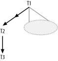
The tree has one root, exactly one table with no join to its primary key. All nodes other than the root node have a single downward-pointing arrow linking them to a detail node above, but any node can be at the top end of any number of downward-pointing arrows.
All joins have downward-pointing arrows (joins that are unique on one end).
Outer joins are unfiltered, pointing down, with only outer joins below outer joins.
The question that the query answers is basically a question about the entity represented at the top (root) of the tree or about aggregations of that entity.
The other tables just provide reference data stored elsewhere for normalization.
I have called queries that meet these criteria simple queries, although, as you saw in Chapter 6, they can contain any number of joins and can be quite tricky to optimize in rare special cases of near-ties between filter ratios or when hidden join filters exist.
Queries do not always fit this standard, simple form. When they do not, I call such queries complex. As I will demonstrate in this chapter, some complex queries result from mistakes: errors in the database design, the application design, or in the implementation. Often, these types of mistakes make it easy to write incorrect queries. In this chapter, you’ll learn about anomalies that you might see in query diagrams that can alert you to the strong possibility of an error in a query or in design. You will also see how to fix these functional or design defects, sometimes fixing performance as a side effect. These fixes usually convert the query to simple form, or at least to a form that is close enough to simple form to apply the methods shown earlier in this book.
Some complex queries go beyond any form I have yet explained how to
diagram, using subqueries, views, or set operations such as UNION and UNION
ALL. These complex queries are usually fine functionally and are
fairly common, so you need a way to diagram and optimize them, which you
can do by extending the earlier methods for simple queries.
Abnormal Join Diagrams
If your query contains only simple tables (not views), no
subqueries, and no set operations such as UNION, you can always produce some sort of
query diagram by applying the methods of Chapter 5. However, sometimes a diagram
has abnormal features that fail to match the usual join-tree template
described earlier. I will describe these anomalies one by one and
discuss how to handle each one.
To illustrate the anomalies, I will show partial query diagrams, in which the parts of the diagram that are not significant to the discussion are hidden behind gray clouds. This focuses attention on the part that matters, and makes clearer the generality of the example. As a convention, I will show links to parts of the join skeleton hidden behind the clouds in gray when they are not significant to the discussion. The number of gray links or even the existence of gray links is not significant to the examples, just illustrative of the potential existence of added joins in real cases. Occasionally, I will have black links to hidden parts of the query skeleton. The existence of the black links is significant to the discussion, but the hidden part of the query skeleton is not.
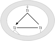
Cyclic Join Graphs
How do you handle join skeletons that do not map to a simple tree but contain links that close a loop somewhere in the skeleton? There are several cases for which you might encounter such a diagram. In the following sections, I will discuss four cases with distinct solutions.
Tip
Graph theory is the branch of mathematics that describes abstract entities, called graphs, that consist of links and nodes, such as the query diagrams this book uses. In graph theory, a cyclic graph has links that form a closed loop. In the following examples, up to Figure 7-8, note that a real or implied loop exists in the diagram, making these graphs cyclic.
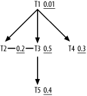
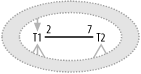
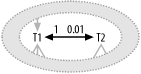
Case 1: Two one-to-one master tables share the same detail table
Figure 7-1 illustrates the first case, in which a single foreign key joins to primary keys in two different master tables.
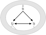
In this case, you can infer that the SQL itself looks something like this:
SELECT ... FROM ...T1, ... T2, ... T3, ... WHERE ... T1.FKey1=T2.PKey2 AND T1.FKey1=T3.PKey3 AND T2.PKey2=T3.PKey3 ...
Here, I have named the single foreign key that points to both
tables from T1 FKey1, and I have named the primary keys
of T2 and T3 PKey2 and PKey3, respectively. With all three of
these joins explicit in the SQL, the cyclic links are obvious, but
note that you could have left any one of these links out of the
query, and transitivity (if
a=b and
b=c, then
a=c) would imply the
missing join condition. If one of these joins were left out, you
might diagram the same query in any of the three forms shown in
Figure 7-2.
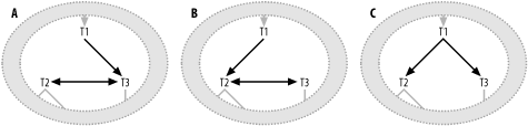
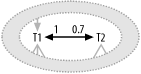
Note that in versions A and B of this query you can infer the
missing arrow from the fact that the link between T2 and T3 has an arrowhead on both ends, and an
arrow at both ends implies a one-to-one join. Version C, on the
other hand, looks exactly like a plain-vanilla join tree, and you
would not realize that it had cyclic joins unless you happened to
notice that T1 used the same
foreign key to join to both T2
and T3.
When you have one-to-one tables, cyclic joins like the one in
Figure 7-1 are common.
These are not a functional problem, though I will later describe
issues to consider whenever you encounter a one-to-one join. Instead
of being a problem, you can see such joins as an opportunity. If you
have already reached T1, it is
useful to have the choice of either T2 or T3 next, since either might have the
better filter ratio or provide access to good filters lower down the
tree. If you reach either T2 or
T3 in the join order before you
reach T1, it is also useful to
have the option to join one-to-one to the other (from T2 to T3, or from T3 to T2). This enables you to reach any filter
the other table might have, without joining to T1 first. Without the horizontal link, you
could join from T2 to T3 or vice versa, only through T1, at likely higher cost.
Some optimizers are written cleverly enough to use transitivity to fill in a missing join condition even if it is left out and take advantage of the extra degrees of freedom that are provided in the join order. However, to be safe, it is best to make all three joins explicit if you notice that two joins imply a third by transitivity. At the least, you should make explicit in your SQL statement any join you need for the optimum plan you find.
There exists a special case in which the one-to-one
tables shown as T2 and T3 are the same table! In this case, each
row from T1 joins to the same row
of T2 twice, a clear
inefficiency. The obvious cause, having the same table name repeated
twice in the FROM clause and
aliased to both T2 and T3, is unlikely, precisely because it is
too obvious to go unnoticed. However, a join to the same table twice
can happen more subtly and be missed in code review. For example, it
can happen if a synonym or simple view hides the true identity of
the underlying table behind at least one of the aliases in the
query. Either way, you are clearly better off eliminating the
redundant table reference from the query and shifting all column
references and further downward joins to the remaining
alias.
Case 2: Master-detail tables each hold copies of a foreign key that points to the same third table’s primary key
Figure 7-3 shows
the second major case with cyclic joins. Here, identical foreign
keys in T1 and T2 point to the same primary key value in
T3.
This time, the SQL looks like this:
SELECT ... FROM ...T1, ... T2, ... T3, ... WHERE ... T1.FKey1=T2.PKey2 AND T1.FKey2=T3.PKey3 AND T2.FKey2=T3.PKey3 ...
In this SQL statement, I name the foreign keys that point from
T1 to T2 and T3 FKey1 and FKey2, respectively. By transitivity, the
foreign-key column T2.FKey2 has
the same value as T1.FKey, since
both join to T3.PKey3. I name the
primary keys of T2 and T3 PKey2 and PKey3, respectively. The most likely
explanation for T1 and T2 joining to the same table, T3, on its full primary key is that
T1 and T2 contain redundant foreign keys to that
table. In this scenario, the FKey2 column in the detail table T1 has denormalized data from its master
table T2. This data always
matches the FKey2 value in the
matching master row of T2.
Tip
Alternatively, the FKey2
values are supposed to match but sometimes do not, since
denormalized data is notoriously likely to get out of sync.
Chapter 10
covers the pros and cons of denormalization in cases like this.
Briefly, if the denormalization is justifiable, it is possible that
the extra link in the query diagram will buy you access to a better
execution plan. However, it is more likely that the denormalization
is a mistake, with more cost and risk than benefit. Eliminating the
denormalization would eliminate the foreign key FKey2 in T1, thus eliminating the link from
T1 to T3 and making the query diagram a
tree.
Case 3: Two-node filter (nonunique on both ends) between nodes is already linked through normal joins
Figure
7-4 shows the third major case with cyclic joins. This time,
you have normal downward arrows from T1 to T2 and T3, but you also have some third, unusual
join condition between T2 and
T3 that does not involve the
primary key of either table.
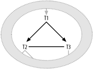
Tip
Since neither primary key is involved in the join
between T2 and T3, the link between these two has no
arrow on either end.
The SQL behind Figure 7-4 looks like this:
SELECT ...
FROM ...T1, ... T2, ... T3,...
WHERE ... T1.FKey1=T2.PKey2
AND T1.FKey2=T3.PKey3
AND T2.Col2<IsSomeHowComparedTo>T3.Col3 ...For example, if T1 were on
the Orders table, having joins to
Customers, T2, and Salespersons, T3, a query might request orders in which
customers are assigned to different regions than the salesperson
responsible for the order:
SELECT ... FROM Orders T1, Customers T2, Salespersons T3 WHERE T1.Customer_ID=T2.Customer_ID AND T1.Salesperson_ID=T3.Salesperson_ID AND T2.Region_ID!=T3.Region_ID
Here, the condition T2.Region_ID!=T3.Region_ID is technically
a join, but it is better to view it as a filter condition that
happens to require rows from two different tables before it can be
applied. If you ignore the unusual, arrow-free link between T2 and T3, you will reach T1 before you can apply the two-node
filter on Region_ID. The only
allowed join orders, which avoid directly following the unusual join
between T2 and T3, are:
(T1, T2, T3) |
(T1, T3, T2) |
(T2, T1, T3) |
(T3, T1, T2) |
Any join order other than these four (such as (T2, T3, T1)) would create a disastrous
many-to-many explosion of rows after reaching the second table,
almost a Cartesian product of the rows in T2 and T3. All of these join orders reach
T1 by the first or second table,
before you have both T2 and
T3. These join orders therefore
follow only the two ordinary many-to-one joins between the detail
table T1 and its master tables
T2 and T3.
The unusual, two-node filter acts like no filter at all when you reach the first of the two filtered tables, then it acts like an ordinary filter, discarding some fraction of rows, when you reach the second of the two tables. Viewed in this way, handling this case is fairly straightforward: consider the filter to be nonexistent (or at least not directly accessible) until you happen to join to one of the filtered tables as a matter of course. However, as soon as you have joined to either end of the two-node filter, the other node suddenly acquires a better filter ratio and becomes more attractive to join to next.
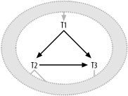
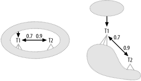
Figure 7-5 shows
a specific example with a two-node filter, in which the fraction of
rows from the ordinary joins from T1 to T2 and T3 that meet the additional two-node
filter condition is 0.2. In this case, you would initially choose a
join order independent of the existence of the two-node filter,
following only ordinary join links. However, as soon as you happened
to join to either T2 or T3, the other would have its former filter
ratio (1.0 for T2 and 0.5 for
T3) multiplied by 0.2, becoming
much more attractive for future joins.
Follow the normal procedure to tune Figure 7-5, ignoring the
two-node filter between T2 and
T3 until you reach one of those
tables as a matter of course. The driving table is T1, followed by T4, the table with the best ordinary
filter downstream of T1. T3 has the next best ordinary filter
available, with the filter ratio 0.5, so it follows next in the join
order. Now, you have a choice between T2 and T5 next in the join order, but T2 has at last seen the two-node filter
activated, since you just reached T3, so it has a more effective filter
ratio, at 0.2, than T5 has, and
you join to T2 next. The final
best join order is (T1, T4, T3, T2,
T5).
Tip
The join to T2 in the
just-completed example is an ordinary join, following nested loops
into the primary-key index on T2 from the foreign key pointing down
from T1. Avoid nested loops
into a table on the two-node filter. Referring back to the SQL
just before Figure
7-5, you would be far better off reaching the Customers table on nested loops from the
join T1.Customer_ID=T2.Customer_ID than on
the two-node filter T2.Region_ID!=T3.Region_ID.
Case 4: Multipart join from two foreign keys is spread over two tables to a multipart primary key
Finally, Figure
7-6 shows the fourth major case with cyclic joins. Here are
two unusual joins to T3, neither
using the whole primary key of that table nor the primary keys of
the tables on the other ends of these joins. If such cases of
failing to join to the whole primary key on at least one end of each
join are “wrongs,” then Case 4 is usually a case in which two wrongs
make a right!
In a situation such as that shown in Figure 7-6, the SQL typically looks like this:
SELECT ... FROM ...T1, ... T2, ... T3, ... WHERE ... T1.FKey1=T2.PKey2 AND T1.FKey2=T3.PKeyColumn1 AND T2.FKey3=T3.PkeyColumn2 ...
Such SQL typically arises when you have a two-part primary key
on T3 and the two-part foreign
key is somehow distributed over two tables in a master-detail
relationship.
A concrete example will clarify this case. Consider
data-dictionary tables called Tables, Indexes, Table_Columns, and Index_Columns. You might choose a two-part
primary key for Table_Columns of
(Table_ID, Column_Number), where
Column_Number designates the
place that table column holds in the natural column order of the
table—1 for the first column,
2 for the second, and so on. The
Indexes table would have a
foreign key to Tables on the
Table_ID column, and the Index_Columns table would also have a
two-part primary key, (Index_ID,
Column_Number). The Column_Number value in the Index_Columns has the same meaning as
Column_Number in Table_Columns: the place the column holds
in the natural order of table columns (not its place in the index
order, which is Index_Position).
If you knew the name of an index and wished to know the list of
column names that make up the index in order of Index_Position, you might query:
SELECT TC.Column_Name FROM Indexes Ind, Index_Columns IC, Table_Columns TC WHERE Ind.Index_Name='EMPLOYEES_X1' AND Ind.Index_ID=IC.Index_ID AND Ind.Table_ID=TC.Table_ID AND IC.Column_Number=TC.Column_Number ORDER BY IC.Index_Position ASC
If the condition on Index_Name had a filter ratio of 0.0002,
the query diagram, leaving off the join ratios, would look like
Figure 7-7.

Here, two wrongs (i.e., two joins that fail to find a full
primary key on either side) combine to make a right when you
consider the joins to TC
together, because combined they reach the full primary key of that
table. You can transform the diagram of this uncommon case
generically, as in Figure
7-8.
If you follow the rule of thumb to join either to or from full
primary keys, the best join order for Figure 7-7 becomes clear.
Drive from the filter on Ind and
follow the upward link to IC.
Only then, after reaching both parts of the primary key to TC, should you join to TC. This is, in fact, the best execution
plan for the example. The rule of thumb in these cases is only to
follow these unusual links into a multipart primary key once the
database has reached all the upward nodes necessary to use the full
primary key.
Cyclic join summary
The following list summarizes the way in which you should treat each of the four cyclic join types just described:
- Case 1: Two one-to-one master tables share the same detail table
This is an opportunity for tuning, increasing the degrees of freedom in the join order, but you should consider options spelled out later in this chapter for handling one-to-one joins.
- Case 2: Master-detail tables each hold copies of a foreign key pointing to the same third table’s primary key
This too is an opportunity to increase the degrees of freedom in the join order, but the case implies denormalization, which is usually not justified. Remove the denormalization if you have the choice, unless the benefit to this or some other query justifies the denormalization. Chapter 10 describes further how to evaluate the trade offs involved in denormalization.
Tip
Throughout this book, I recommend ideal actions under the assumption that you have complete power over the application, the database design, and the SQL. I’ve also tried to recommend compromise solutions that apply when you have more limited control. Sometimes, though, such as when you see unjustified denormalization in an already-released database design that you do not own or even influence, the only compromise is to do nothing.
- Case 3: Two-node filter (nonunique on both ends) between nodes is already linked through normal joins
Treat this uncommon case as no filter at all until you reach one of the nodes. Then, treat the other node as having a better filter ratio for purposes of finding the rest of the join order.
- Case 4: Multipart join from two foreign keys is spread over two tables to a multipart primary key
Perform this join into the primary key only when you have both parts of the key.
Disconnected Query Diagrams
Figure 7-9 shows two cases of disconnected query diagrams: query skeletons that fail to link all the query tables into a single connected structure. In each of these cases, you are in a sense looking at two independent queries, each with a separate query diagram that you can optimize in isolation from the other query.
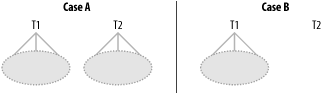
In Case A, I show a query that consists of two
independent-appearing queries that each have joins. In Case B, I show
an otherwise ordinary-looking query that has one of its tables (table
T2) disconnected from the join tree
(i.e., not joined to any other table). Each of the two cases maps to
two independent queries being run within a single query. What happens
when you combine independent, disconnected queries into a single
query? When two tables are combined in a single query without any join
condition, the database returns a Cartesian product: every possible combination of the
rows from the first table with the rows from the second table. In the
case of disconnected query diagrams, think of the query result
represented by each independent query skeleton (or isolated node) as
being its own virtual table. From this point of view, you can see that
the database will return all combinations of rows from the two
independent queries. In short, you’ll get a Cartesian product.
When confronted with a Cartesian product such as the one shown in Figure 7-9, you should investigate the reason behind it. Once you learn the reason, you can decide which of the following courses of action to take, depending on which of four cases of disconnected queries you have:
- Case 1: Query is missing a join that would connect the disconnected parts
- Case 2: Query combines two independent queries, each returning multiple rows
Eliminate this Cartesian product by running the independent queries separately.
- Case 3: One of the independent queries is a single-row query
Consider separating the queries to save bandwidth from the database, especially if the multirow independent query returns many rows. Execute the single-row query first.
- Case 4: Both of the independent queries are single-row queries
Keep the query combined, unless it is confusing or hard to maintain.
Before you turn a disconnected query into two separate queries, consider whether the developer might have inadvertently left a join out of the single query. Early in the development cycle, the most common cause of disconnected query diagrams is developers simply forgetting some join clause that links the disconnected subtrees. When this is the case, you should add in the missing join condition, after which you will no longer have a disconnected tree. Whenever one of the tables in one tree has a foreign key that points to the primary key of the root node of the other tree, that join was almost certainly left out accidentally.
If each independent query returns multiple rows, the number of combinations will exceed the number of rows you would get if you just ran the two queries separately. However, the set of combinations from the two contains no more information than you could get if you ran these separately, so the work of generating the redundant data in the combinations is just a waste of time, at least from the perspective of getting raw information. Thus, you might be better off running the two queries separately.
Rarely, there are reasons why generating the combinations in a Cartesian product is at least somewhat defensible, from the perspective of programming convenience. However, you always have workarounds that avoid the redundant data if the cost is unjustified.
Tip
If you were concerned only with physical I/O, the Cartesian product would likely be fine, since the redundant rereads of data from the repeated query would almost certainly be fully cached after the first read. I have actually heard people defend long running examples of queries like this based on the low physical I/O they saw! Queries like this are a great way to burn CPU and generate enormous logical I/O if you ever need to do so for some sort of stress test or other laboratory-type study, but they have no place in business applications.
If one of the independent queries returns just a single row, guaranteed, then at least the Cartesian product is safe and is guaranteed to return no more rows than the larger independent query would return. However, there is still potentially a small network cost in combining the queries, because the select list of the combined query might return the data from the smaller query many times over, once for each row that the multirow query returns, requiring more redundant bytes than if you broke up the queries. This bandwidth cost is countered somewhat with network-latency savings: the combined query saves you round trips to the database over the network, so the best choice depends on the details. If you do not break the up queries, the optimum plan is straightforward: just run the optimum plan for the single-row query first. Then, in a nested loop that executes only once, run the optimum plan for the multirow query. This combined execution plan costs the same as running the two queries separately. If, instead, you run the plan for the multirow query first, a nested-loops plan would require you to execute the plan for the single-row query repeatedly, once for every row of the other query.
Combining a single-row query with a multirow query is sometimes
convenient and justified. There is a special case, matching the right
half of Figure 7-9, in
which the single-row query is simply a read of the only row of
isolated table T2, which has no
joins at all. A Cartesian product with an isolated table is sometimes
useful to pick up site parameters stored in a single-row parameters
table, especially when these parameters show up only in the WHERE clause, not in the SELECT list. When the query does not return
data from the parameters table, it is actually cheaper to run the
correctly combined query than to run separate queries.
An even rarer case guarantees that both isolated queries return a single row. It is fully justified and safe, from the performance perspective, to combine the queries in this case, which lacks any of the dangers of the other cases. However, from the programming and software-maintenance perspective, it might be confusing to combine queries like this, and the savings are generally slight.
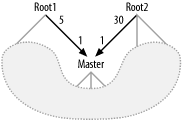
Query Diagrams with Multiple Roots
Figure
7-10 shows an example of a query diagram that violates the
one-root expectation. This case is akin to the previous case
(disconnected query diagrams). Here, for each row in the Master table shown that satisfies the query
condition, the query will return all combinations of matching details
from Root1 and Root2. Given the detail join ratios, you can
expect all combinations of 5 Root1
details with 30 Root2 details, for
150 combination rows for each matching Master row. These 150 combination rows
contain no more original data than the 5 Root1 details combined with the 30 Root2 details, so it is faster to read these
5 and 30 rows separately, avoiding the Cartesian product. While
disconnected query diagrams generate a single large Cartesian product,
multiple root nodes generate a whole series of smaller Cartesian products, one for each matching master
row.
There are four possible causes of a query diagram with multiple roots. The following list details these causes, and describes their solutions:
- Case 1: Missing condition
The query is missing a condition that would convert one of the root detail tables into a master table, making a one-to-many join one-to-one.
Solution: Add the missing join condition.
- Case 2: Many-to-many Cartesian product
The query represents a many-to-many Cartesian product per master-table row between detail tables that share a master table. This appears in the guise of detail join ratios greater than 1.0 from a single shared master to two different root detail tables.
Solution: Eliminate this Cartesian product by separating the query into independent queries that read the two root detail tables separately.
- Case 3: Detail join ratio less than 1.0
One of the root detail tables joins to the shared master table with a detail join ratio less than 1.0.
Solution: Although this is not a problem for performance, consider separating the query parts or turning one of the query parts into a subquery, for functional reasons.
- Case 4: Table used only for existence check
One of the root detail tables supplies no data needed in the
SELECTlist and is included only as an existence check.Solution: Convert the existence check to an explicit subquery.
Case 1: Missing join conditions
Most often, the appearance of a second root node
points to some missing join condition that would convert one of the
root nodes to a master node. Figure 7-11 shows this
transformation, where the join from Master to Root1 has been converted to a one-to-one
join by the addition (or recognition) of some extra condition on
Root1 (renamed R1) that ensures that the database will
find at most one row in R1 for
every row in Master. This is
particularly likely when R1
contains time-interval detail data (such as a varying tax rate) that
matches a master record (such as taxing entity) and the addition of
a date condition (such as requesting the
current tax rate) makes the join
one-to-one.
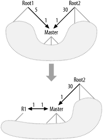
Often, the condition that makes the join one-to-one is already there, and you find a combination of a many-to-one join and an apparent filter that just cancels the detail join ratio.
Tip
In the example, the filter ratio for such a filter would be
0.2, or 1/5, where the detail join ratio to Root1 was 5.
Alternatively, the condition that makes the join one-to-one might be missing from the query, especially if development happens in a test system where the one-to-many relationship is hidden.
Tip
The previous example of a varying tax rate illustrates this. In a development environment, you might find records only for the current rate, obscuring the error of leaving out the date condition on the rates table.
Whether the condition that makes the join one-to-one was missing or was just not recognized as being connected with the join, you should include the condition and recognize it as part of the join, not as an independent filter condition. Such a missing join condition is particularly likely when you find that the foreign key for one of the root tables pointing downward to a shared master table is also part of the multipart primary key of that root table.
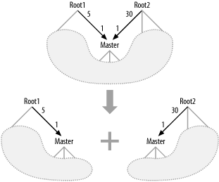
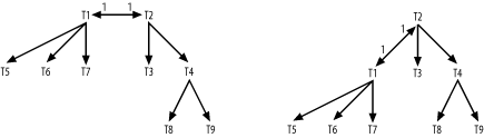
Case 2: Breaking the Cartesian product into multiple queries
Figure
7-12 shows another solution to the multiroot-query-diagram
problem. This solution is akin to running explicitly separate
queries in the disconnected query diagram (discussed earlier),
breaking up the Cartesian product and replacing it with the two
separate sets. In the example, this replaces a query that would
return 150 rows per Master row
with two queries that, combined, return 35 rows per Master row. Whenever you have one-to-many
relationships from a master table to two different detail root
tables, you can get precisely the same underlying data, with far
fewer rows read and with separate queries, as illustrated. Since the
result takes an altered form, you will also need to change the
underlying application logic to handle the new form.
Case 3: Root detail tables that are usually no more than one-to-one
Figure
7-13 shows a case of multiple roots in which performance of
the query, unaltered, is not a problem. Since the detail join ratio
from Master to Root1 is 0.5, you see no Cartesian
explosion of rows when you combine matching Root1 with Root2 records for the average matching
Master record. You can treat
Root1 as if it were a downward
join, even favoring it as if it had a filter ratio enhanced by 0.5
for the filtering join, following the special-case rules in Chapter 6 for detail join ratios
less than 1.0.
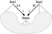
Although this query is no problem for tuning, it might still
be incorrect. The one-to-zero or one-to-many join from Master to Root1 evidently usually finds either the
one-to-zero or the one-to-one case, leading to a well-behaved
Cartesian product. However, as long as the join is ever one-to-many,
you must consider that the result might return a Cartesian product
with repeats for a given row of Root2. Since this case is rare, it is all
too likely that the query was actually designed and tested to return
results that map one-to-one with rows from Root2, and the application might not even
work in the other rare case.
Warning
The rarer the one-to-many case is, the more likely it is that this case has been neglected in the application design.
For example, if the application will alter Root2 data after reading it out with this
query and attempt to post the alterations back to the database, the
application must consider which copy of a repeated Root2 row should get posted back to the
database. Should the application warn an end user that it attempted
to post inconsistent copies? If the application aggregates Root2 data from the query, does it avoid
adding data from repeated Root2
rows?
Case 4: Converting an existence check to an explicit subquery
One solution to the functional problem that Figure 7-13 represents is
already shown in Figure
7-12: just break up the query into two queries. Another
solution, surprisingly often, is to isolate the branch to Root1 into a subquery, usually with an
EXISTS condition. This solution
works especially easily if the original query did not select columns
from Root1 (or any of the tables
joined below it through hidden gray links in Figure 7-13). In this
relatively common special case, you are really interested only in
whether a matching row in Root1
exists and perhaps matches some filter conditions, not in the
contents of that row or the number of matches (beyond the first)
that might exist. Later in this chapter, you will see how to diagram
and tune queries with subqueries like this.
Joins with No Primary Key
I use join links without arrows on either end to show
joins that involve no primary key on either side of the join. In
general, these represent unusual many-to-many joins, although in some
cases they might usually be many-to-zero or many-to-one. If they are
never many-to-many, then you simply failed to recognize the unique
condition and you should add an arrow to the unique side of the join.
If they are at least sometimes many-to-many, you have all the same
problems (and essentially the same solutions) you have with query
diagrams that have multiple root nodes. Figure 7-14 shows a
many-to-many join between T1 and
T2, where the detail join ratio on
each end is greater than 1.0. (Master join ratios exist only on the
unique end of a link, with an arrow, so this link has two detail join
ratios.)
This case turns out to be much more common than the previous
examples of abnormal join diagrams. Although it shares all the same
possible problem sources and solutions as the case of multiple root
nodes, the overwhelming majority of many-to-many joins are simply due
to missing join conditions. Begin by checking whether filter
conditions already in the query should be treated as part of the join,
because they complete specification of the full primary key for one
end of the join. Example
5-2 in Chapter 5 was
potentially such a case, with the condition OT.Code_Type='ORDER_STATUS' needed to
complete the unique join to alias OT. Had I treated that condition as merely a
filter condition on alias OT, the
join to OT would have looked
many-to-many. Even if you do not find the missing part of the join
among the query filter conditions, you should suspect that it was
mistakenly left out of the query.
This case of missing join conditions is particularly
common when the database design allows for multiple entity types or
partitions within a table and the developer forgets to restrict the
partition or type as part of the query. For example, the earlier
example of a Code_Translations
table has distinct types of translation entities for each Code_Type, and leaving off the condition on
Code_Type would make the join to
Code_Translations many-to-many.
Often, testing fails to find this problem early, because even though
the database design might allow for multiple types or partitions, the
test environment might have just a single type or partition to begin
with, a state of affairs developers might take for granted. Even when
there are multiple types or partitions in the real data, the other,
more selective part of the key might, by itself, be usually unique.
This is both good and bad luck: while it prevents the missing join
condition from causing much immediate trouble, it also makes the
problem much harder to detect and correct, and lends a false sense
that the application is correct. Finding and correcting the missing
join condition might help performance only slightly, by making the
join more selective, but it can be a huge service if it fixes a really
pernicious hidden bug.
By direct analogy with query diagrams that have multiple root nodes, the solutions to many-to-many joins map to similar solutions to diagrams with multiple root nodes.
One-to-One Joins
You have probably heard the joke about the old fellow who complains he had to walk five miles to school every morning uphill both ways. In a sense, one-to-one joins turn this mental picture on its head: for the heuristic rules of which table to join next, one-to-one joins are downhill both ways! As such, these joins create no problem for tuning at all, and these are the least troublesome of the unusual features possible in a query diagram. However, they do sometimes point to opportunities to improve database design, if you are at a point in the development cycle when database design is not yet set in stone. It is also useful to have a standard way to represent one-to-one joins on a query diagram, so I will describe ways to represent these cases.
One-to-one join to a subset table
Figure 7-15
shows a typical one-to-one join embedded in a larger query. While
many-to-many joins have detail join ratios on both ends, one-to-one
joins have master join ratios on both ends. The master join ratios
in the example show that the join between T1 and T2 is really one-to-zero or one-to-one;
the one-to-zero case happens for 30% of the rows in T1.
Since this is an inner join, the one-to-zero cases between
T1 and T2 make up a hidden join filter, which you
should handle as described at the end of Chapter 6. Also note that this
might be a case of a hidden cyclic join, as often happens when a
master table joins one-to-one with another table. If you have a
detail table above T1, as implied
by the gray link upward, and if that detail table joins to T1 by the same unique key as used for the
join to T2, then you have, by
transitivity, an implied join from the detail table to T2. Figure 7-16 shows this
implied link in gray. Refer back to cyclic joins earlier in this
chapter for how to handle this case.
Whether or not you have a cyclic join, though, you might have
an opportunity to improve the database design. The case in Figure 7-16 implies a set of
entities that map one-to-one with T1 and a subset of those same entities
that map one-to-one with T2, with
T2 built out of T1’s primary key and columns that apply
only to that subset. In this case, there is no compelling need to
have two tables at all; just add the extra columns to T1 and leave them null for members of the
larger set that do not belong to the subset! Occasionally, there are
good reasons why development prefers a two-table design for
convenience in a situation like this. However, from the perspective
of tuning, combining these two comparably sized tables is almost
always helpful, so at least give it some thought if you have any
chance to influence the database design.
Exact one-to-one joins
Figure 7-17 shows an especially compelling case for combining the tables into a single table, when possible. Here, the master join ratios are each exactly 1.0, and the relationship between the tables is exactly one-to-one. Both tables, therefore, map to the same set of entities, and the join is just needless expense compared to using a combined table.
The only reason, from a performance perspective, to separate these tables is if queries almost always need just the data from one or the other and rarely need to do the join. The most common example of this is when one of the tables has rarely needed data, compared to the other. In that case, especially if the rarely needed data takes up a lot of space per row and the tables are large, you might find that the better compactness of the commonly queried table, resulting in a better cache-hit ratio, will (barely) justify the cost of the rarely needed joins. Even from a functional or development perspective, it is likely that the coding costs of adding and deleting rows for both tables at once—and, sometimes, updating both at once—are high. You might prefer to maintain a single, combined table. Usually, when you see an exact one-to-one join, it is a result of some bolted-on new functionality that requires new columns for existing entities, and some imagined or real development constraint prevented altering the original table. When possible, it is best to solve the problem by eliminating that constraint.
One-to-one join to a much smaller subset
At the other end of the spectrum, you have the case
shown in Figure 7-18,
a one-to-zero or one-to-one join that is almost always one-to-zero.
Here, the case for separating the tables is excellent. The tiny
subset of entities represented by T2 might have different optimization needs
than the superset represented by T1. Probably, T1 is usually queried without the join to
T2, and, in these cases, it is
useful that it excludes the inapplicable columns in T2 and has only the indexes that make
sense for the common entities. Here, the hidden join filter
represented by the small master join ratio on the T2 side of the join is excellent. It is so
good, in fact, that you might choose to drive from an unfiltered
full table scan of T2 and still
find the best path to the rest of the data. Such an execution plan
would be hard to approximate, without creating otherwise useless
indexes, if you combined these tables into a single table.
Here, the key issue is not to neglect to take into account the
hidden join filter from T1 to
T2, either driving from the
T2 side of the query or reaching
it as soon as possible to pick up the hidden filter early.
One-to-one joins with hidden join filters in both directions
Figure 7-19 shows a rare case of a [zero or one]-to-[zero or one] join, which filters in both directions. If one-to-one joins are downhill in both directions, then [zero or one]-to-[zero or one] joins are steeply downhill in both directions. However, unless data is corrupt (i.e., one of the tables is missing data), this rare case probably implies that yet a third table exists, or should exist, representing a superset of these two overlapping sets. If you find or create such a table, the same arguments as before apply for combining it with one or both of the subset tables.
![A [zero or one]-to-[zero or one] join](http://imgdetail.ebookreading.net/data/2/0596005733/0596005733__sql-tuning__0596005733__httpatomoreillycomsourceoreillyimages11711.png)
Conventions to display one-to-one joins
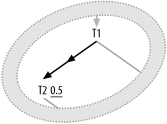
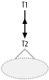
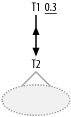
It helps to have agreed-upon conventions for laying out query diagrams. Such conventions aid tuning intuition by presenting key information uniformly. Single-ended arrows always point down, by convention. Figure 7-20 shows two alternatives that work well for one-to-one joins that lie below the root detail table. The first alternative emphasizes the two-headed arrow, placing neither node above the other. The second alternative emphasizes the usual downward flow of reference links from the root detail table. Either alternative works well, as long as you remember that both directions of a one-to-one join are, in the usual sense, downward.
For this case, in which both joined tables are below the root,
keep in mind that if the one-to-one tables actually share a common
primary key, then the link from above into T1 could probably just as easily be to
T2, by transitivity, unless it is
to some alternate unique key on T1 not shared by T2. This is the implied cyclic-join case
illustrated with form B in Figure 7-2.
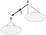
Figure 7-21 illustrates alternate diagrams for one-to-one joins of tables that both qualify as root detail tables (i.e., they have no joins from above), where at least one of the directions of the one-to-one join shows a master join ratio less than 1.0. Again, you can emphasize the one-to-one link with a horizontal layout, or you can emphasize which table is larger (and which direction of the join is “more downhill”) by placing the node with the larger master join ratio higher. The node with the larger master join ratio represents a table with more rows in this [zero or one]-to-[zero or one] join.
![Alternate diagram methods for [zero or one]-to-[zero or one] root detail tables](http://imgdetail.ebookreading.net/data/2/0596005733/0596005733__sql-tuning__0596005733__httpatomoreillycomsourceoreillyimages11715.png)
Figure 7-22 illustrates a case similar to Figure 7-21, but with nodes that are perfectly one-to-one (tables that always join successfully). Again, you can emphasize the equal nature of the join directions by laying the nodes out horizontally. Alternatively, you can just choose a direction that makes a more balanced-looking tree, which fits better on the page, placing the node with deeper branches at the top. The choice in this case matters least, as long as you remember that both join directions are virtually downhill, regardless of how you lay out the diagram.
Outer Joins
Almost always, the sense and purpose of an outer join is that it prevents loss of desired information from the joined-from table, regardless of the contents of the outer-joined table. Abnormal outer joins, which I describe in the following sections, generally imply some contradiction of this reason behind the outer join.
Filtered outer joins
Consider Figure
7-23, with an outer join to a table with a filter condition.
In the outer case, the case where a T1 row has no matching T2 row, the database assigns null to every
T2 column in the result.
Therefore, except for T2.SomeColumn IS
NULL, almost any filtering condition on T2 would specifically exclude a result row
that comes from the outer case of the outer join.
Even conditions such as T2.Unpaid_Flag != 'Y' or NOT T2.Unpaid_Flag = 'Y', which you might
expect to be true for the outer case, are not.
Warning
Databases interpret nulls in a nonintuitive way,
when it comes to conditions in the WHERE clause. If you think of the null
as representing “unknown” with regard to a column of table, rather
than the much more common “does-not-apply,” you can begin to
understand how databases treat nulls in conditions. Except for
questions specifically about whether the column is null, almost
anything you can ask about an unknown returns the answer
“unknown,” which is in fact the truth value
of most conditions on nulls. From the perspective of rejecting
rows for a query, the database treats the truth value “unknown”
like FALSE, rejecting rows with
unknown truth values in the WHERE clause. And, while NOT FALSE = TRUE, you’ll find that NOT “unknown” = “unknown”!
Since most filters on the outer table discard the outer case of an outer join, and since the whole purpose of an outer join is to preserve such cases, you need to give careful attention to any filter on an outer table. One of the following scenarios applies, and you should take the time to determine which:
The filter is one of the rare filters, such as
SomeColumn IS NULL, that can returnTRUEfor null column values inserted in the outer case, and the filter is functionally correct.The developer did not intend to reject the outer case, and the filter condition must be removed.
The filter condition was meant to reject the outer case, and the join might as well be an inner join. When this is the case, there is no functional difference between the query with the join expressed as an outer or as an inner join. However, by expressing it formally as an inner join, you give the database more degrees of freedom to create execution plans that might perform this join in either direction. When the best filter is on the same side of the join as the formerly-outer-joined table, the added degrees of freedom might enable a better execution plan. On the other hand, converting the join to an inner join might just enable the optimizer to make a mistake it would have avoided with an outer join. Outer joins are one way to constrain join orders when you consciously wish to do so, even when you do not need to preserve the outer case.
The filter condition was intended, but it should be part of the join! With the filter condition made part of the join, you order the database: “For each detail-table row, provide the matching row from this table that fits this filter, if any; otherwise, match with an all-null pseudorow.”
Let’s consider the first scenario in further depth. Consider the query:
SELECT ...
FROM Employees E
LEFT OUTER JOIN Departments D
ON E.Department_ID=D.Department_ID
WHERE D.Dept_Manager_ID IS NULLWhat is the query really asking the database in this case? Semantically, this requests two rather distinct rowsets: all employees that have no department at all and all employees that have leaderless departments. It is possible that the application actually calls for just two such distinct rowsets at once, but it is more likely that the developer did not notice that such a simple query had such a complex result, and did not intend to request one of those rowsets.
Consider a slightly different example:
SELECT ... FROM Employees E
LEFT OUTER JOIN Departments D
ON E.Department_ID=D.Department_ID
WHERE D.Department_ID IS NULLOn the surface, this might seem to be a bizarre query, because
the primary key (Department_ID)
of Departments cannot be null.
Even if the primary key could be null, such a null key value could
never successfully join to another table with a join like this
(because the conditional expression NULL =
NULL returns the truth value “unknown”). However, since
this is an outer join, there is a reasonable interpretation of this
query: “Find the employees that fail to have matching departments.”
In the outer case of these outer joins, every column of Departments, including even mandatory
nonnull columns, is replaced by a null, so the condition D.Department_ID IS NULL is true only in the outer case. There
is a much more common and easier-to-read way to express this
query:
SELECT ...
FROM Employees E
WHERE NOT EXISTS (SELECT *
FROM Departments D
WHERE E.Department_ID=D.Department_ID)Although the NOT EXISTS
form of this sort of query is more natural and easier to read and
understand, the other form (preferably commented carefully with
explanation) has its place in SQL tuning. The advantage of
expressing the NOT EXISTS
condition as an outer join followed by PrimaryKey IS NULL is that it allows more
precise control of when in the execution plan the join happens and
when you pick up the selectivity of that condition. Usually,
NOT EXISTS conditions evaluate
after all ordinary joins, at least on Oracle. This is the one
example in which a filter (that is not part of the outer join) on an
outer-joined table is really likely to have been deliberate and
correct.
Note
In the older-style SQL Server outer-join notation, the combination of outer join and is-null condition does not work. For example, adapting the example to SQL Server’s notation, you might try this:
SELECT ... FROM Employees E, Departments D WHERE E.Department_ID*=D.Department_ID AND D.Department_ID IS NULL
However, the result will not be what you wanted! Recall that
SQL Server interprets all filter conditions on the outer-joined
table as part of the join. SQL Server will attempt to join to
Departments that have null
primary keys (i.e., null values of D.Department_ID). Even if such rows
exist in violation of correct database design, they can never
successfully join to Employees,
because the equality join cannot succeed for null key values.
Instead, the query will filter no rows, returning all employees,
with all joins falling into the outer case.
Outer joins leading to inner joins
Consider Figure 7-24, in which an outer join leads to an inner join.
In old-style Oracle SQL, you express such a join as follows:
SELECT ... FROM Table1 T1, Table2 T2, Table3 T3 WHERE T1.FKey2=T2.PKey2(+) AND T2.FKey3=T3.PKey3
In the outer case for the first join, the database will
generate a pseudorow of T2 with
all null column values, including the value of T2.FKey3. However, a null foreign key can
never successfully join to another table, so that row representing
the outer case will be discarded when the database attempts the
inner join to T3. Therefore, the
result of an outer join leading to an inner join is precisely the
same result you would get with both joins being inner joins, but the
result is more expensive, since the database discards the rows that
fail to join later in the execution plan. This is always a mistake.
If the intent is to keep the outer case, then replace the outer join
to an inner join with an outer join leading to another outer join.
Otherwise, use an inner join leading to an inner join.
Outer joins pointing toward the detail table
Consider Figure 7-25, in which the midlink arrow shows the outer join that points toward the detail table.
In the new-style ANSI join notation, this might look like this:
SELECT ...
FROM Departments D
LEFT OUTER JOIN Employees E
ON D.Department_ID=E.Department_IDOr, in older Oracle notation:
SELECT ... FROM Departments D, Employees E WHERE D.Department_ID=E.Department_ID(+)
Or, in older SQL Server notation:
SELECT ... FROM Departments D, Employees E WHERE D.Department_ID*=E.Department_ID
In any of these, what does this query semantically ask? It asks something like: “Give me all the employees that have departments (the inner case), together with their department data, and also include data for departments that don’t happen to have employees (the outer case).” In the inner case, the result maps each row to a detail entity (an employee who belongs to a department), while in the outer case, the result maps each row to a master entity (a department that belongs to no employee). It is unlikely that such an incongruous mixture of entities would be useful and needed from a single query, so queries like this, with outer joins to detail tables, are rarely correct. The most common case of this mistake is a join to a detail table that usually offers zero or one detail per master, and that is only rarely many-to-one to the master table. Developers sometimes miss the implications of the rare many-to-one case, and it might not come up in testing.
Outer joins to a detail table with a filter
Figure 7-26 shows an outer join to a detail table that also has a filter condition. Occasionally, two wrongs do make a right. An outer join to a detail table that also has a filter might be doubly broken, suffering from the problems described in the last two subsections. Sometimes, the filter cancels the effect of the problematic outer join, converting it functionally to an inner join. In such cases, you need to avoid removing the filter unless you also make the outer join inner.
The most interesting case Figure 7-26 can illustrate
is the case in which the filter makes sense only in the context of
the outer join. This is the case in which the filter condition on
T1 is true only in the outer
case—for example, T1.Fkey_ID IS
NULL. (Here, T1.Fkey_ID
is the foreign key pointing to T2.PKey_ID in the diagrammed join.) Like
the earlier example of a join-key-value IS
NULL condition (on the primary key, in the earlier case),
this case is equivalent to a NOT
EXISTS subquery. As in the earlier example, this unusual
alternative expression for the NOT
EXISTS condition sometimes offers a useful additional
degree of control over when in the execution plan the database
performs the join and discards the rows that do not meet the
condition. Since all inner-joined rows are discarded by the IS NULL condition, it avoids the usual
problem of outer joins to a detail table: the mixing of distinct
entities behind rows from the inner and the outer cases of the join.
Two wrongs make a right!
Queries with Subqueries
Almost all real-world queries with subqueries impose a special kind of condition on the rows in the outer, main query; they must match or not match corresponding rows in a related query. For example, if you need data about departments that have employees, you might query:
SELECT ...
FROM Departments D
WHERE EXISTS (SELECT NULL
FROM Employees E
WHERE E.Department_ID=D.Department_ID)Alternatively, you might query for data about departments that do not have employees:
SELECT ... FROM Departments D
WHERE NOT EXISTS (SELECT NULL
FROM Employees E
WHERE E.Department_ID=D.Department_ID)The join E.Department_ID=D.Department_ID in each of
these queries is the correlation join, which matches between tables in
the outer query and the subquery. The EXISTS query has an alternate, equivalent
form:
SELECT ... FROM Departments D WHERE D.Department_ID IN (SELECT E.Department_ID FROM Employees E)
Since these forms are functionally equivalent, and since the diagram should not convey a preconceived bias toward one form or another, both forms result in the same diagram. Only after evaluating the diagram to solve the tuning problem should you choose which form best solves the tuning problem and expresses the intended path to the data.
Diagramming Queries with Subqueries
Ignoring the join that links the outer query with the
subquery, you can already produce separate, independent query diagrams
for each of the two queries. The only open question is how you should
represent the relationship between these two diagrams, combining them
into a single diagram. As the EXISTS form of the earlier query makes
clear, the outer query links to the subquery through a join: the
correlation join. This join has a special property: for each
outer-query row, the first time the database succeeds in finding a
match across the join, it stops looking for more matches, considers
the EXISTS condition satisfied, and
passes the outer-query row to the next step in the execution plan.
When it finds a match for a NOT
EXISTS correlated subquery, it stops with the NOT EXISTS condition that failed and
immediately discards the outer-query row, without doing further work
on that row. All this behavior suggests that a query diagram should
answer four special questions about a correlation join, questions that do not apply to
ordinary joins:
Is it an ordinary join? (No, it is a correlation join to a subquery.)
Which side of the join is the subquery, and which side is the outer query?
Is it expressible as an
EXISTSor as aNOT EXISTSquery?How early in the execution plan should you execute the subquery?
When working with subqueries and considering these questions, remember that you still need to convey the properties you convey for any join: which end is the master table and how large are the join ratios.
Diagramming EXISTS subqueries
Figure
7-27 shows my convention for diagramming a query with an
EXISTS-type subquery (which might
be expressed by the equivalent IN
subquery). The figure is based on the earlier EXISTS subquery:
SELECT ... FROM Departments D
WHERE EXISTS (SELECT NULL
FROM Employees E
WHERE E.Department_ID=D.Department_ID)For the correlation join (known as a
semi-join when applied to an EXISTS-type subquery) from Departments to Employees, the diagram begins with the
same join statistics shown for Figure 5-1.
Like any join, the semi-join that links the inner query to the
outer query is a link with an arrowhead on any end of the join that
points toward a primary key. Like any join link, it has join ratios
on each end, which represent the same statistical properties the
same join would have in an ordinary query. I use a midpoint arrow to point from the outer-query
correlated node to the subquery correlated node. I place an
E beside the midpoint arrow to
show that this is a semi-join for an EXISTS or IN subquery.
In this case, as in many cases with subqueries, the subquery part of the diagram is a single node, representing a subquery without joins of its own. Less frequently, also as in this case, the outer query is a single node, representing an outer query with no joins of its own. The syntax is essentially unlimited, with the potential for multiple subqueries linked to the outer query, for subqueries with complex join skeletons of their own, and even for subqueries that point to more deeply nested subqueries of their own.
The semi-join link also requires up to two new numbers to convey properties of the subquery for purposes of choosing the best plan. Figure 7-27 shows both potential extra values that you sometimes need to choose the optimum plan for handling a subquery.
The first value, next to the E (20 in
Figure 7-27) is the
correlation preference ratio.
The correlation preference ratio is the ratio of
I/E.
E is the estimated or measured runtime of the
best plan that drives from the outer query to the subquery
(following EXISTS logic).
I is the estimated or measured runtime of the
best plan that drives from the inner query to the outer query
(following IN logic). You can
always measure this ratio directly by timing both forms, and doing
so is usually not much trouble, unless you have many subqueries
combined. Soon I will explain some rules of thumb to estimate
I/E more or less
accurately, and even a rough estimate is adequate to choose a plan
when, as is common, the value is either much less than 1.0 or much
greater than 1.0. When the correlation preference ratio is greater
than 1.0, choose a correlated subquery with an EXISTS condition and a plan that drives
from the outer query to the subquery.
The other new value is the subquery adjusted filter ratio (0.8 in Figure 7-27), next to the detail join ratio. This is an estimated value that helps you choose the best point in the join order to test the subquery condition. This applies only to queries that should begin with the outer query, so exclude it from any semi-join link (with a correlation preference ratio less than 1.0) that you convert to the driving query in the plan.
Tip
If you have more than one semi-join with a correlation preference ratio less than 1.0, you will drive from the subquery with the lowest correlation preference ratio, and you still need adjusted filter ratios for the other subqueries.
Before I explain how to calculate the correlation preference
ratio and the subquery adjusted filter ratios, let’s consider when
you even need them. Figure
7-28 shows a partial query diagram for an EXISTS-type subquery, with the root detail
table of the subquery on the primary-key end of the
semi-join.
Here, the semi-join is functionally no different than an
ordinary join, because the query will never find more than a single
match from table M for any given
row from the outer query.
Tip
I assume here that the whole subtree under M is normal-form
(i.e., with all join links pointing downward toward primary keys),
so the whole subquery maps one-to-one with rows from the root
detail table M of the
subtree.
Since the semi-join is functionally no different than an
ordinary join, you can actually buy greater degrees of freedom in
the execution plan by explicitly eliminating the EXISTS condition and merging the subquery
into the outer query. For example, consider this query:
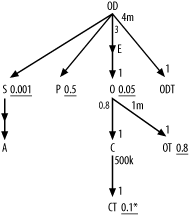
SELECT<Columns from outer query only>FROM Order_Details OD, Products P, Shipments S, Addresses A, Code_Translations ODT WHERE OD.Product_ID = P.Product_ID AND P.Unit_Cost > 100 AND OD.Shipment_ID = S.Shipment_ID AND S.Address_ID = A.Address_ID(+) AND OD.Status_Code = ODT.Code AND ODT.Code_Type = 'Order_Detail_Status' AND S.Shipment_Date > :now - 1 AND EXISTS (SELECT null FROM Orders O, Customers C, Code_Translations OT, Customer_Types CT WHERE C.Customer_Type_ID = CT.Customer_Type_ID AND CT.Text = 'Government' AND OD.Order_ID = O.Order_ID AND O.Customer_ID = C.Customer_ID AND O.Status_Code = OT.Code AND O.Completed_Flag = 'N' AND OT.Code_Type = 'ORDER_STATUS' AND OT.Text != 'Canceled') ORDER BY<Columns from outer query only>
Using the new semi-join notation, you can diagram this as shown in Figure 7-29.
If you simply rewrite this query to move the table joins and conditions in the subquery into the outer query, you have a functionally identical query, since the semi-join is toward the primary key and the subquery is one-to-one with its root detail table:
SELECT<Columns from the original outer query only>FROM Order_Details OD, Products P, Shipments S, Addresses A, Code_Translations ODT, Orders O, Customers C, Code_Translations OT, Customer_Types CT WHERE OD.Product_Id = P.Product_Id AND P.Unit_Cost > 100 AND OD.Shipment_Id = S.Shipment_Id AND S.Address_Id = A.Address_Id(+) AND OD.Status_Code = ODT.Code AND ODT.Code_Type = 'Order_Detail_Status' AND S.Shipment_Date > :now - 1 AND C.Customer_Type_Id = CT.Customer_Type_Id AND CT.Text = 'Government' AND OD.Order_Id = O.Order_Id AND O.Customer_Id = C.Customer_Id AND O.Status_Code = OT.Code AND O.Completed_Flag = 'N' AND OT.Code_Type = 'ORDER_STATUS' AND OT.Text != 'Canceled' ORDER BY<Columns from the original outer query only>
I have indented this version to make obvious the simple transformation from one to the other in this case. The query diagram is also almost identical, as shown in Figure 7-30.
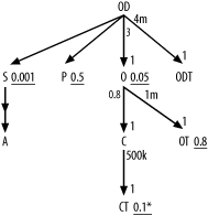
This new form has major additional degrees of freedom,
allowing, for example, a plan joining to moderately filtered
P after joining to highly
filtered O but before joining to
the almost unfiltered node OT.
With the original form, the database would be forced to complete the
whole subquery branch before it could consider joins to further
nodes of the outer query. Since merging the subquery in cases like
this can only help, and since this creates a query diagram you
already know how to optimize, I will assume for the rest of this
section that you will merge this type of subquery. I will only
explain diagramming and optimizing other types.
In theory, you can adapt the same trick for merging EXISTS-type subqueries with the semi-join
arrow pointing to the detail end of the join too, but it is harder
and less likely to help the query performance. Consider the earlier
query against departments with the EXISTS condition on Employees:
SELECT ...
FROM Departments D
WHERE EXISTS (SELECT NULL
FROM Employees E
WHERE E.Department_ID=D.Department_ID)These are the problems with the trick in this direction:
The original query returns at most one row per master table row per department. To get the same result from the transformed query, with an ordinary join to the detail table (
Employees), you must include a unique key of the master table in theSELECTlist and perform aDISTINCToperation on the resulting query rows. These steps discard duplicates that result when the same master record has multiple matching details.When there are several matching details per master row, it is often more expensive to find all the matches than to halt a semi-join after finding just the first match.
Therefore, you should rarely transform semi-joins to ordinary joins when the semi-join arrow points upward, except when the detail join ratio for the semi-join is near 1.0 or even less than 1.0.
To complete a diagram for an EXISTS-type subquery, you just need rules
to estimate the correlation preference ratio and the subquery
adjusted filter ratio. Use the following procedure to estimate the
correlation preference ratio:
For the semi-join, let D be the detail join ratio, and let M be the master join ratio. Let S be the best (smallest) filter ratio of all the nodes in the subquery, and let R be the best (smallest) filter ratio of all the nodes in the outer query.
If D x S<M / R, set the correlation preference ratio to (D x S)/(M x R).
Otherwise, if S>R, set the correlation preference ratio to S/R.
Otherwise, let E be the measured runtime of the best plan that drives from the outer query to the subquery (following
EXISTSlogic). Let I be the measured runtime of the best plan that drives from the inner query to the outer query (followingINlogic). Set the correlation preference ratio to I/E. When Steps 2 or 3 find an estimate for the correlation preference ratio, you are fairly safe knowing which direction to drive the subquery without measuring actual runtimes.Tip
The estimated value from Step 2 or Step 3 might not give the accurate runtime ratio you could measure. However, the estimate is adequate as long as it is conservative, avoiding a value that leads to an incorrect choice between driving from the outer query or the subquery. The rules in Steps 2 and 3 are specifically designed for cases in which such safe, conservative estimates are feasible.
When Steps 2 and 3 fail to produce an estimate, the safest and easiest value to use is what you actually measure. In this range, which you will rarely encounter, finding a safe calculated value would be more complex than is worth the trouble.
Once you have found the correlation preference ratio, check whether you need the subquery adjusted filter ratio and determine the subquery adjusted filter ratio when you need it:
If the correlation preference ratio is less than 1.0 and less than all other correlation preference ratios (in the event that you have multiple subqueries), stop. In this case, you do not need a subquery preference ratio, because it is helpful only when you’re determining when you will drive from the outer query, which will not be your choice.
If the subquery is a single-table query with no filter condition, just the correlating join condition, measure q (the rowcount with of the outer query with the subquery condition removed) and t (the rowcount of the full query, including the subquery). Set the subquery adjusted filter ratio to t/q. (In this case, the
EXISTScondition is particularly easy to check: the database just looks for the first match in the join index.)Otherwise, for the semi-join, let D be the detail join ratio. Let s be the filter ratio of the correlating node (i.e., the node attached to the semi-join link) on the detail, subquery end.
If D ≤ 1, set the subquery adjusted filter ratio equal to s / D.
Otherwise, if s x D<1, set the subquery adjusted filter ratio equal to (D-1+(s x D))/D.
Otherwise, set the subquery adjusted filter ratio equal to 0.99. Even the poorest-filtering
EXISTScondition will avoid actually multiplying rows and will offer a better filtering power per unit cost than a downward join with no filter at all. This last rule covers these better-than-nothing (but not much better) cases.
Tip
Like other rules in this book, the rules for calculating the correlation preference ratio and the subquery adjusted filter ratio are heuristic. Because exact numbers are rarely necessary to choose the right execution plan, this carefully designed, robust heuristic leads to exactly the right decision at least 90% of the time and almost never leads to significantly suboptimal choices. As with many other parts of this book, a perfect calculation for a complex query would be well beyond the scope of a manual tuning method.
Try to see if you understand the rules to fill in the correlation preference ratio and the subquery adjusted filter ratio by completing Figure 7-31, which is missing these two numbers.
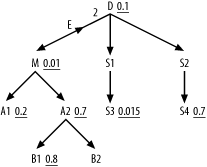
Check your own work against this explanation. Calculate the correlation preference ratio:
Set D=2 and M=1 (implied by its absence from the diagram). Set S=0.015 (the best filter ratio of all those in the subquery, on the table
S3, which is two levels below the subquery root detail tableD). Then set R=0.01, which is the best filter for any node in the tree under and including the outer-query’s root detail tableM.Find D x S=0.03 and M x R=0.01, so D / S>M x R. Move on to Step 3.
Since S>R, set the correlation preference ratio to S/R, which works out to 1.5.
To find the subquery adjusted filter ratio, follow these steps:
Note that the correlation preference ratio is greater than 1, so you must proceed to Step 2.
Note that the subquery involves multiple tables and contains filters, so proceed to Step 3.
Find D=2, and find the filter ratio on node
D, s=0.1.Note that D>1, so proceed to Step 5.
Calculate s x D=0.2, which is less than 1, so you estimate the subquery adjusted filter ratio as (D-1+(s x D))/D = (2-1+(0.1 x 2))/2 = 0.6.
In the following section on optimizing EXISTS subqueries, I will illustrate
optimizing the completed diagram, shown in Figure 7-32.
Diagramming NOT EXISTS subqueries
Subquery conditions that you can express with NOT EXISTS or NOT
IN are simpler than EXISTS-type subqueries in one respect: you
cannot drive from the subquery outward to the outer query. This
eliminates the need for the correlation preference ratio. The
E that indicates an EXISTS-type subquery condition is replaced
by an N to indicate a NOT EXISTS-type subquery condition, and
the correlation join is known as an anti-join rather than a
semi-join, since it searches for the case when the join to rows from
the subquery finds no match.
It turns out that it is almost always best to express NOT EXISTS-type subquery conditions with
NOT EXISTS, rather than with
NOT IN. Consider the following
template for a NOT IN
subquery:
SELECT ...
FROM ... Outer_Anti_Joined_Table Outer
WHERE...
AND Outer.Some_Key NOT IN (SELECT Inner.Some_Key
FROM ... Subquery_Anti_Joined_Table Inner WHERE<Conditions_And_Joins_On_Subquery_Tables_Only>)
...You can and should rephrase this in the equivalent NOT EXISTS form:
SELECT ...
FROM ... Outer_Anti_Joined_Table Outer
WHERE...
AND Outer.Some_Key IS NOT NULL
AND NOT EXISTS (SELECT null
FROM ... Subquery_Anti_Joined_Table Inner WHERE<Conditions_And_Joins_On_Subquery_Tables_Only>
AND Outer.Some_Key = Inner.Some_Key)Tip
To convert NOT IN to
NOT EXISTS without changing
functionality, you need to add a not-null condition on the
correlation join key in the outer table. This is because the
NOT IN condition amounts to a
series of not-equal-to conditions joined by OR, but a database does not evaluate
NULL!=
<SomeValue> as true, so the
NOT IN form rejects all
outer-query rows with null correlation join keys. This fact is not
widely known, so it is possible that the actual intent of such a
query’s developer was to include, in the query result, these rows
that the NOT IN form subtly
excludes. When you convert forms, you have a good opportunity to
look for and repair this likely bug.
Both EXISTS-type and
NOT EXISTS-type subquery
conditions stop looking for matches after they find the first match,
if one exists. NOT EXISTS
subquery conditions are potentially more helpful early in the
execution plan, because when they stop early with a found match,
they discard the matching row, rather than retain it, making later
steps in the plan faster. In contrast, to discard a row with an
EXISTS condition, the database
must examine every potentially matching row and rule them all out, a
more expensive operation when there are many details per master
across the semi-join. Remember the following rules, which compare
EXISTS and NOT EXISTS conditions that point to detail
tables from a master table in the outer query:
An unselective
EXISTScondition is inexpensive to check (since it finds a match easily, usually on the first semi-joined row it checks) but rejects few rows from the outer query. The more rows the subquery, isolated, would return, the less expensive and the less selective theEXISTScondition is to check. To be selective, anEXISTScondition will also likely be expensive to check, since it must rule out a match on every detail row.A selective
NOT EXISTScondition is inexpensive to check (since it finds a match easily, usually on the first semi-joined row it checks) and rejects many rows from the outer query. The more rows the subquery, isolated, would return, the less expensive and the more selective theEXISTScondition is to check. On the other hand, unselectiveNOT EXISTSconditions are also expensive to check, since they must confirm that there is no match for every detail row.
Since it is generally both more difficult and less rewarding
to convert NOT EXISTS subquery
conditions to equivalent simple queries without subqueries, you will
often use NOT EXISTS subqueries
at either end of the anti-join: the master-table end or the
detail-table end. You rarely need to search for alternate ways to
express a NOT EXISTS
condition.
Since selective NOT EXISTS
conditions are inexpensive to check, it turns out to be fairly
simple to estimate the subquery adjusted filter ratio:
Measure q (the rowcount of the outer query with the
NOT EXISTSsubquery condition removed) and t (the rowcount of the full query, including the subquery). Let C be the number of tables in the subqueryFROMclause (usually one, forNOTEXISTSconditions).
Tuning Queries with Subqueries
As for simple queries, optimizing complex queries with subqueries turns out to be straightforward, once you have a correct query diagram. Here are the steps for optimizing complex queries, including subqueries, given a complete query diagram:
Convert any
NOT INcondition into the equivalentNOT EXISTScondition, following the earlier template.If the correlation join is an
EXISTS-type join, and the subquery is on the master end of that join (i.e., the midpoint arrow points down), convert the complex query to a simple query as shown earlier, and tune it following the usual rules for simple queries.Otherwise, if the correlation join is an
EXISTS-type join, find the lowest correlation preference ratio of all theEXISTS-type subqueries (if there is more than one). If that lowest correlation preference ratio is less than 1.0, convert that subquery condition to the equivalentINcondition and express any otherEXISTS-type subquery conditions using theEXISTScondition explicitly. Optimize the noncorrelatedINsubquery as if it were a standalone query; this is the beginning of the execution plan of the whole query. Upon completion of the noncorrelated subquery, the database will perform a sort operation to discard duplicate correlation join keys from the list generated from the subquery. The next join after completing this first subquery is to the correlating key in the outer query, following the index on that join key, which should be indexed. From this point, treat the outer query as if the driving subquery did not exist and as if this first node were the driving table of the outer query.If all correlation preference ratios are greater than or equal to 1.0, or if you have only
NOT EXISTS-type subquery conditions, choose a driving table from the outer query as if that query had no subquery conditions, following the usual rules for simple queries.As you reach nodes in the outer query that include semi-joins or anti-joins to not-yet-executed subqueries, treat each entire subquery as if it were a single, downward-hanging node (even if the correlation join is actually upward). Choose when to execute the remaining subqueries as if this virtual node had a filter ratio equal to the subquery adjusted filter ratio.
Tip
Because correlated subqueries stop at the first row matched, if any, they avoid the row-multiplying risk of normal upward joins and can only reduce the running rowcount. However, since they must often examine many rows to have this filtering effect, the correct value of the subquery adjusted filter ratio often makes this virtual node equivalent to an almost unfiltered node in benefit/cost ratio.
Wherever you place the correlated join in the join order following Step 5, you then immediately perform the rest of that correlated subquery, optimizing the execution plan of that subquery with the correlating node as the driving node of that independent query. When finished with that subquery, return to the outer query and continue to optimize the rest of the join order.
As an example, consider Figure 7-32, which is Figure 7-31 with the correlation preference ratio and the subquery adjusted filter ratio filled in.
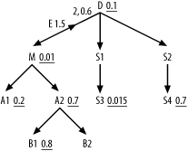
Since the correlated join is EXISTS-type, Step 1 does not apply. Since
the midpoint arrow of the semi-join points upward, Step 2 does not
apply. The lowest (the only) correlation preference ratio is 1.5 (next
to the E), so Step 3 does not apply. Applying
Step 4, you find that the best driving node in the outer query is
M. Applying Step 5, choose between
downward joins to A1 and A2 with filter ratios of 0.2 and 0.7,
respectively, or a virtual downward join to the virtual node
representing the whole subquery, with a virtual filter ratio of 0.6.
A1 is the best of these three
candidates, with the best filter ratio, so join to it next. Finding
nothing downstream of A1, you next
find the subquery as the next-best choice in the join order (again
applying Step 5), so perform the semi-join to D.
Applying Step 6, having begun the subquery, you must finish it,
starting from D as the driving
node. Following simple-query rules within that subquery, next join to
S1, S3, S2,
and S4, in that order. Returning to
the outer query, applying the usual rules for simple queries, you find
the remainder of the join order, A2, B1,
B2. The whole optimum join order,
including the semi-join, is then (M, A1, D,
S1, S3, S2, S4, A2, B1,
B2).
Queries with Views
A view can make an arbitrarily complex query look like a simple table from the point of view of a person writing a query using the view. When multiple queries will share much underlying SQL, shared, reusable views can be a powerful mechanism to reduce complexity in application code. Unfortunately, simply hiding steps from the application developer does not reduce the underlying complexity of the steps to reach actual data. On the contrary, hiding complexity from the developer will more likely than not increase the difficulty of the tuning problem that the optimizer, whether automated or human, must overcome to find a fast execution plan. In this discussion, I refer to two types of queries important to the tuning problem:
- View-defining queries
These are the queries that underlie views (i.e., the queries used to create views with
CREATE VIEW<ViewName>AS<ViewDefiningQuery>).- View-using queries
These are queries you tune and that the database must actually execute. These queries reference views in their
FROMclause (for example,SELECT ... FROM View1V1, View2 V2,... WHERE ...).
Warning
I am frequently asked to tune, or to estimate performance of, a
view-defining query without having the list of view-using queries that
use the defined view. I am also asked to tune view-using queries
without knowing the view-defining query. Neither request is realistic:
no view-defining query more complex than SELECT
<ListOfSimpleColumns> FROM
<SingleTable> will perform well in
every possible view-using query, and no view-using query will perform
well if the view-defining query interferes with an efficient path to
the required data.
For a given view, you must know and tune every view-using query to know that a view-defining query is completely correct in context. You must know the view-defining query of every view used to know that a view-using query is correct.
When you tune SQL, views tend to add complexity in three ways:
You must translate a view-using query into an equivalent query against real tables to create and optimize a join diagram.
Queries against views often contain unnecessary or redundant nodes in the query skeleton. Each view carries with it a whole view-defining query, complete with a subtree that includes all view-defining nodes and joins. Use of the view implies use of the entire subtree. However, the developer using the view often needs only a few of the view columns and could skip a number of the nodes and joins in the view-defining query if she wrote the equivalent query against simple tables. When the application requires all the nodes in the view, the view-using query still might be hitting those nodes redundantly, joining to the same rows of the same underlying tables in multiple hidden contexts. An example of this will follow in Section 7.3.2.2.
Sometimes, view-using queries cannot be expressed simply as equivalent queries against simple tables. Usually, the cases in which the view-using query returns different results from a simple table query are rare corner cases. However, the correct results in the corner cases are usually not the results the view-using query gets! When a view-using query does not decompose well into a simple, perfectly equivalent simple query against tables, performance almost always suffers, and the corner cases that define the view-specific functional behavior are usually wrong. Nevertheless, to fix the performance with an almost equivalent simple query against tables does require at least a slight change in functionality, and you must exercise caution not to introduce a bug. (You will more often than not be fixing a bug, rather than creating one, but the new bugs will be noticed more!) An example of this will follow in Section 7.3.2.1.
Diagramming View-Using Queries
Diagramming view-using queries is relatively straightforward, though sometimes tedious:
Create a diagram of each view-defining query as if it were a standalone query. Each query diagram that defines a view should be normal, in the sense that it has a single root detail table and has only downward-hanging many-to-one joins from that top node, in a tree structure. If a view-defining query does not map to a normal query skeleton, the queries that use the view will most likely perform badly and return incorrect results. Treat the primary key of the root detail table for the view-defining query as the virtual primary key of the whole view.
Create a query diagram of the view-using query as if each view were just a simple table. A join to a view should have an arrow on the view end (and you should place the view on the lower end of the link) only if the join is to the virtual primary key of the view. Show filter conditions on the view in the view-using query symbolically, as the letter F, without bothering to work out the filter ratio yet. Draw a dotted circle around each view node.
Expand the view-using query diagram of Step 2, replacing each node that represents a view with the entire view-defining query diagram from Step 1 with a dotted curve around the view-defining query subtree. Any join from above will attach to the view-defining subtree at its root detail node. Joins that reach downward from the view can attach to any node of the view, depending on which table of the view-defining query provided the foreign key (in the view-defining
SELECTlist) of the join. Any filter condition on the view becomes a filter condition on the appropriate node of the view-defining query, depending on which node’s column the filter condition restricts. Work out the actual filter ratio for each of these conditions in the usual way (expanding the symbolic F in the initial query diagram). As needed, combine filter ratios from the view-defining queries and from the view-using queries, when these two queries place distinct filters on the same nodes.
These rules probably strike you as abstract and complex, but an example should make the process much clearer. Consider these two view definitions:
CREATE VIEW Shipment_V AS
SELECT A.Address_ID Shipment_Address_ID, A.Street_Addr_Line1
Shipment_Street_Address_Line1, A.Street_Addr_Line2
Shipment_Street_Address_Line2, A.City_Name Shipment_City_Name,
A.State_Abbreviation Shipment_State, A.ZIP_Code Shipment_ZIP,
S.Shipment_Date, S.Shipment_ID
FROM Shipments S, Addresses A
WHERE S.Address_ID = A.Address_ID
CREATE VIEW Recent_Order_V AS
SELECT O.Order_ID, O.Order_Date, O.Customer_ID,
C.Phone_Number Customer_Main_Phone, C.First_Name Customer_First_Name,
C.Last_Name Customer_Last_Name,
C.Address_ID Customer_Address_ID, OT.Text Order_Status
FROM Orders O, Customers C, Code_Translations OT
WHERE O.Customer_ID = C.Customer_ID
AND O.Status_Code = OT.Code
AND OT.Code_Type = 'ORDER_STATUS'
AND O.Order_Date > SYSDATE - 366Step 1 calls for query diagrams of these two view-defining queries, as shown in Figure 7-33. These query diagrams were created by following the method described in Chapter 5 and using the same filter ratio and join ratio statistics as for the related example shown in Figure 5-5.
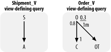
The view-using query, then, is:
SELECT OV.Customer_Main_Phone, C.Honorific, OV.Customer_First_Name,
OV.Customer_Last_Name, C.Suffix, OV.Customer_Address_ID,
SV.Shipment_Address_ID, SV.Shipment_Street_Address_Line1,
SV.Shipment_Street_Address_Line2, SV.Shipment_City_Name,
SV.Shipment_State, SV.Shipment_Zip, OD.Deferred_Shipment_Date,
OD.Item_Count, ODT.Text, P.Product_Description, SV.Shipment_Date
FROM Recent_Order_V OV, Order_Details OD, Products P, Shipment_V SV,
Code_Translations ODT, Customers C
WHERE UPPER(OV.Customer_Last_Name) LIKE :last_name||'%'
AND UPPER(OV.Customer_First_Name) LIKE :first_name||'%'
AND OD.Order_ID = OV.Order_ID
AND OV.Customer_ID = C.Customer_ID
AND OD.Product_ID = P.Product_ID(+)
AND OD.Shipment_ID = SV.Shipment_ID(+)
AND OD.Status_Code = ODT.Code
AND ODT.Code_Type = 'ORDER_DETAIL_STATUS'
ORDER BY OV.Customer_ID, OV.Order_ID Desc, SV.Shipment_ID, OD.Order_Detail_IDProceeding to Step 2, create the initial query diagram as if the views were simple tables, as shown in Figure 7-34.

Replace each view node in Figure 7-34 with the earlier
query diagrams for the view-defining queries in Figure 7-33, with each
view-defining query skeleton surrounded by a dotted curve to show the
boundaries of the view. Attach the view-defining query skeletons to
the rest of the full query diagram at the appropriate table nodes,
depending on which table in the view definition contains the joining
key. Normally, any joins into the view from above will be to the root
detail table of the view-defining query. However, master-table nodes
that hang down from the view (for example, the node labeled C in Figure 7-34) can attach to any
node of the view-defining skeleton, depending on which table contains
the foreign key that points to that master node. Add explicit,
numerical filter ratios to any nodes of the query skeleton that have
filters either in the view-defining query or in the view-using query.
In Figure 7-33, the
filter ratio 0.3 next to node O
comes from the filter in the view-defining query, while the filter
ratio 0.0002 next to node C comes
from the view-using query conditions on the customer’s first and last
names.
The result for the example should look like Figure 7-35, in which I have
added an asterisk to the leftmost C
node to clarify the distinction between the two otherwise identically
labeled nodes. Again, I borrow the same statistics for the filter on
customer name as in the similar example shown earlier in Figure 5-5, to arrive at the
filter ratio of 0.0002 next to the C within the rightmost view skeleton.
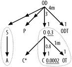
This completes the diagram you need to proceed to actual tuning of the view-using query, to determine whether either the view-defining query or the view-using query must change to enable the optimum plan.
Tuning Queries with Views
Normally, the optimum execution plan for the view-using query is exactly the execution plan you would find for the corresponding query diagram against simple tables. However, there are four special problems you might have to resolve:
Some joins to complex views are hard to express precisely as simple joins to simple tables. In particular, outer joins to views that have joins in the view-defining queries are complex to express with simple joins. This problem affects the example, and I will explain it in detail in Section 7.3.2.1.
Some views reference precisely the same rows of the same table as another table in the view-using query, making redundant work for the database that you should eliminate. This happens for the nodes labeled
C*andCin Figure 7-35, and I’ll discuss this issue further too.The virtue of views, from the perspective of development simplicity, is hiding complexity, but this very virtue makes it all too easy to code redundant joins that would be obvious, and would actually require more work to code, if developers used only simple tables.
Nodes within view-defining queries, and the joins to reach them, are often unnecessary to the required view-using query result.
Using views limits your ability to fully control the execution plan. If you change a view-defining query to improve the execution plan of a view-using query, you might unintentionally harm performance of other queries that use the same view. You can always create a new view just for the use of a single query, but that defeats the code-sharing advantage of views. In general, SQL hints and other changes in the view-using query cannot control how the database accesses tables in the view-defining query. You sometimes must eliminate the use of views to get the execution plan you need.
Outer joins to views
Returning to the earlier example, consider what it
means to have an outer join to the view Shipment_V, which itself is an inner join
between tables Shipments and
Addresses. Since the database
must behave as if there were a real table with precisely the rows
the view would find, the join finds the inner case for Shipment_IDs that exist in Shipments and point to shipments that have
an Address_ID that successfully
joins to Addresses. When the
database cannot successfully join to both Shipments and Addresses, the join to the view is
entirely an outer join (to both tables), even if the initial join to
Shipments could succeed. When
searching for a nested-loops plan, the database cannot know whether
the outer join finds the inner case until it joins successfully to
both tables in the view-defining query.
Unfortunately, this is all too complex for most automated code to handle, so your database might simply give up on a nested-loops plan. Instead, the database code recognizes that no matter how complex the underlying logic might be, it cannot go wrong functionally if, in tricky cases like this, it gets every row from the view-defining query and treats the result like a real table. For the outer join to the view, the database normally performs a sort-merge join or a hash join to that temporarily created table. This is safe enough functionally, but it is usually a disaster for performance, unless the view-defining query is fast as a standalone query.
Warning
As a general rule for performance, avoid outer joins into
any view that is more complex than SELECT
<ListOfSimpleColumns> FROM
<SingleTable>.
Similar problems result for all sorts of joins into views that
have UNIONs or GROUP BYs in the view-defining queries.
However, joining from these views, when they
contain the table you would choose as the driving table of the
query, usually works fine.
Consider, again, the view-using query from the previous
subsection. If you merge the view-defining query for Shipment_V into the view-using query, to
resolve the performance problem with the outer join, you might
expect this result:
SELECT OV.Customer_Main_Phone, C.Honorific, OV.Customer_First_Name,
OV.Customer_Last_Name, C.Suffix, OV.Customer_Address_ID,
A.Address_ID Shipment_Address_ID,
A.Street_Addr_Line1 Shipment_Street_Address_Line1,
A.Street_Addr_Line2 Shipment_Street_Address_Line2,
A.City_Name Shipment_City_Name, A.State_Abbreviation Shipment_State,
A.ZIP_Code Shipment_ZIP, OD.Deferred_Ship_Date, OD.Item_Count,
ODT.Text, P.Prod_Description, S.Shipment_Date
FROM Recent_Order_V OV, Order_Details OD, Products P, Shipments S,
Addresses A, Code_Translations ODT, Customers C
WHERE UPPER(OV.Customer_Last_Name) LIKE :last_name||'%'
AND UPPER(OV.Customer_First_Name) LIKE :first_name||'%'
AND OD.Order_ID = OV.Order_ID
AND OV.Customer_ID = C.Customer_ID
AND OD.Product_ID = P.Product_ID(+)
AND OD.Shipment_ID = S.Shipment_ID(+)
AND S.Address_ID = A.Address_ID(+)
AND OD.Status_Code = ODT.Code
AND ODT.Code_Type = 'ORDER_DETAIL_STATUS'
ORDER BY OV.Customer_ID, OV.Order_ID Desc, S.Shipment_ID, OD.Order_Detail_IDUnfortunately, this does not produce quite the same result as
the original query, because of the peculiarity of the outer join to
the view. Specifically, the original query returns a null Shipment_Date from the view whenever the
entire view, including the join to Addresses, fails to join to Order_Details. Therefore, whenever the
shipment does not have a valid, nonnull Address_ID, the original query returns
null for Shipment_Date, even
though the join to Shipments, by
itself, is valid.
Almost certainly, this peculiar behavior is not what the developer intended and is not functionally necessary, so the form just shown will likely work fine, even better than the original in this corner case. However, any change in functionality, for a performance fix, is dangerous. Therefore, before making a change such as the one just described that merges the view-defining query into the main SQL statement, make certain the new corner-case behavior is correct and warn developers that the change might cause regression tests to return changed results. In the unlikely event that you really need the original behavior, or if you just want to play safe without investigating whether the original corner-case behavior was correct, you can perfectly emulate the original query functionality with this:
SELECT OV.Customer_Main_Phone, C.Honorific, OV.Customer_First_Name,
OV.Customer_Last_Name, C.Suffix, OV.Customer_Address_ID,
A.Address_ID Shipment_Address_ID,
A.Street_Addr_Line1 Shipment_Street_Address_Line1,
A.Street_Addr_Line2 Shipment_Street_Address_Line2,
A.City_Name Shipment_City_Name, A.State_Abbreviation Shipment_State,
A.ZIP_Code Shipment_ZIP, OD.Deferred_Ship_Date, OD.Item_Count,
ODT.Text, P.Prod_Description,DECODE(A.Address_ID, NULL, TO_DATE(NULL),
S.Shipment_Date) Shipment_Date
FROM Recent_Order_V OV, Order_Details OD, Products P, Shipments S,
Addresses A, Code_Translations ODT, Customers C
WHERE UPPER(OV.Customer_Last_Name) LIKE :last_name||'%'
AND UPPER(OV.Customer_First_Name) LIKE :first_name||'%'
AND OD.Order_ID = OV.Order_ID
AND OV.Customer_ID = C.Customer_ID
AND OD.Product_ID = P.Product_ID(+)
AND OD.Shipment_ID = S.Shipment_ID(+)
AND S.Address_ID = A.Address_ID(+)
AND OD.Status_Code = ODT.Code
AND ODT.Code_Type = 'ORDER_DETAIL_STATUS'
ORDER BY OV.Customer_ID, OV.Order_ID Desc,
DECODE(A.Address_ID, NULL, TO_NUMBER(NULL), S.Shipment_ID),
OD.Order_Detail_IDThis query includes two changes that cause the query to return
results as if the join to Shipments produced the outer case whenever
the join to Addresses produced
the outer case. Without the view, the query will treat the join to
Shipments independently from the
join to Addresses. However, the
DECODE expressions in both the
end of the SELECT list and the
middle of the ORDER BY list cause
the inner case of the first join to emulate the outer case of the
join (producing NULL in place of
Shipment_Date and Shipment_ID) whenever the join to Addresses finds the outer case.
Occasionally, you will have some functional need to use a view
in place of simple tables. The most common reason for this is to
work around limitations in autogenerated SQL. Functionally, you
might require some bit of complex SQL syntax that the SQL generator
cannot handle. The common workaround is to bury that complexity in a
view-defining query that you create manually and have the SQL
generator simply treat the view as if it were a simple table, hiding
the complexity from the SQL-generator code. In these cases, you
might not be able to eliminate use of a view, such as I suggest in
the earlier solutions. Your alternate approach is to extend use of
the view, burying more of the SQL in the view definition. For
example, since the previous problem involved an outer join to a
view, you could solve the problem by pulling the outer join into the
view-defining query. With this solution, you would replace use of
Shipment_V with OrderDetail_V, using this view-defining
query:
CREATE VIEW Order_Detail_V AS
SELECT A.Address_ID Shipment_Address_ID,
A.Street_Addr_Line1 Shipment_Street_Address_Line1,
A.Street_Addr_Line2 Shipment_Street_Address_Line2,
A.City_Name Shipment_City_Name, A.State_Abbreviation Shipment_State,
A.ZIP_Code Shipment_ZIP, S.Shipment_Date, S.Shipment_ID,
OD.Deferred_Ship_Date, OD.Item_Count, OD.Order_ID,
OD.Order_Detail_ID, OD.Product_ID, OD.Status_Code
FROM Shipments S, Addresses A, Order_Details OD
WHERE OD.Shipment_ID = S.Shipment_ID(+)
AND S.Address_ID = A.Address_ID(+)The view-using query, using the extended view, then becomes:
SELECT OV.Customer_Main_Phone, C.Honorific, OV.Customer_First_Name,
OV.Customer_Last_Name, C.Suffix, OV.Customer_Address_ID,
ODV.Shipment_Address_ID, ODV.Shipment_Street_Address_Line1,
ODV.Shipment_Street_Address_Line2, ODV.Shipment_City_Name,
ODV.Shipment_State, ODV.Shipment_Zip, ODV.Deferred_Ship_Date,
ODV.Item_Count, ODT.Text, P.Prod_Description, ODV.Shipment_Date
FROM Recent_Order_V OV, Order_Detail_V ODV, Products P,
Code_Translations ODT, Customers C
WHERE UPPER(OV.Customer_Last_Name) LIKE :last_name||'%'
AND UPPER(OV.Customer_First_Name) LIKE :first_name||'%'
AND ODV.Order_ID = OV.Order_ID
AND OV.Customer_ID = C.Customer_ID
AND ODV.Product_ID = P.Product_ID(+)
AND ODV.Status_Code = ODT.Code
AND ODT.Code_Type = 'ORDER_DETAIL_STATUS'
ORDER BY OV.Customer_ID, OV.Order_ID Desc, ODV.Shipment_ID, ODV.Order_Detail_IDRedundant reads in view-using queries
Now, consider the case of the joins in Figure 7-35 to nodes labeled
C* and C. These nodes represent the same table,
with identical join clauses, so any execution plan that hits both
nodes is redundant, reading the same table rows and probably the
same index entries twice. The second, redundant read in every case
should avoid physical I/O, because the first read, likely less than
a millisecond earlier, should place the table or index block safely
at the head of the shared cache. If the execution plan is highly
filtered before it reaches the second, redundant node, the excess
logical I/Os might be negligible, but for large queries or queries
that filter most rows only after such redundant reads, the costs of
the extra logical I/Os are important.
If the developer wrote the query originally against simple tables, this sort of error would be unlikely; he would have to go out of his way to include the redundant join, and the redundancy would be obvious in code review. With views, however, these errors are easy to make and are well hidden.
How do you fix the redundant join to Customers? You have three options:
Add new columns as needed to the
SELECTlist of the view-defining query and use them in place of the column references to the redundant table in the view-using query. This is safe for other queries that use the same view, since it only adds columns and does not change the view-defining query diagram.Eliminate the redundant join from the view-defining query and use only the columns from the simple table node in the view-using query. However, this is dangerous if there are other view-using queries that might require the view columns you eliminated.
Eliminate the use of the view from the view-using query, replacing it with equivalent, nonredundant joins to simple tables.
Unnecessary nodes and joins
Consider the join to node OT in the recent view-using query. The
original view-defining query appears to include that join to support
queries of the order status, but the view-using query does not even
refer to the order status, so you might question whether this node
is necessary. If you did not happen to notice the seemingly unused
node, you could diagnose the unused node if you noticed a join, in
the execution plan, to the primary-key index of this table with no
read of the table itself. Such index-only reads of primary-key
indexes usually point to unnecessary joins.
Safely eliminating these unnecessary joins is not simple,
because they sometimes have functional side effects. Since this is
an inner join, it is at least possible that, even with no filter on
the node, the join itself eliminates rows the query should not
return. This can result either by eliminating rows where Orders.Status_Code IS NULL or where
Status_Code points to invalid
status codes that fail to find a match in the Code_Translations table. The latter
possibility is unlikely or should be eliminated by repairing
referential integrity. However, null foreign keys are common, and if
the column can be null, you should consider adding an explicit
Status_Code IS NOT NULL condition
before eliminating the join, to emulate the implicit filtering
function of the inner join. More likely, the developer using the
view did not even think about the implicit filtering function of the
view, and the implicit filter was entirely unintentional and
undesirable. Therefore, before emulating the old behavior in a
base-table-only query that eliminates the unneeded join, check
whether the old behavior was even correct. If your change will
subtly change behavior, even for the better, warn testers that
regression test results might change for this corner case.
Queries with Set Operations
Occasionally, you must tune multipart queries that use set operations
like UNION, UNION ALL, INTERSECT, and EXCEPT to combine results of two or more
simple queries. The extension of the SQL-diagramming tuning method to
these multipart queries is usually straightforward: diagram and tune
each part independently, as if it were a standalone query. When the
parts are fast, combining the results with set operations generally
works well.
Tip
EXCEPT is the keyword
specified by the ANSI SQL standard for the set operation to find the
difference between two sets. DB2 and SQL Server follow the standard by
supporting EXCEPT. Oracle, however,
uses MINUS for the same
operation, most likely because it supported the operation before the
standard existed.
However, some of these set operations deserve a little extra
discussion. The UNION operation, in
addition to combining the parts, also must sort them and discard
duplicates. This last step is often unnecessary, especially if you
design the parts to avoid duplicates in the first place. In Oracle, you
can replace the UNION operation with
UNION ALL when you determine that
duplicates are either impossible or need not be discarded. In databases
that do not support UNION ALL, you
can skip the duplicate-eliminating step by replacing the single UNION query with two or more simple queries,
combining the results in the application layer, rather than in the
database.
The INTERSECT operation can
generally be profitably replaced with an EXISTS-type subquery
that looks for the matching row that the second part would produce. For
example, if you had two Employees
tables, you might look for shared employee records with this:
SELECT Employee_ID FROM Employees1 INTERSECT SELECT Employee_ID FROM Employees2
You could always replace this INTERSECT query with this:
SELECT DISTINCT Employee_ID
FROM Employees1 E1
WHERE EXISTS (SELECT null
FROM Employees2 E2
WHERE E1.Employee_ID=E2.Employee_ID)Using the methods of Section 7.2, you would then
determine whether this EXISTS
subquery should be expressed in the EXISTS or IN form, or converted to a simple join. Note
that the correlating join conditions become numerous if the SELECT list contains many items. Also note
that INTERSECT will match column
lists with nulls, but a correlation join will not, unless you use join
conditions designed for that purpose. For example, if the
positive-valued foreign key Manager_ID is allowed to be null (but Employee_ID is not), the Oracle equivalent of
this query:
SELECT Employee_ID, Manager_ID FROM Employees1 INTERSECT SELECT Employee_ID, Manager_ID FROM Employees2
is this query:
SELECT DISTINCT Employee_ID, Manager_ID
FROM Employees1 E1
WHERE EXISTS (SELECT null
FROM Employees2 E2
WHERE E1.Employee_ID=E2.Employee_ID
AND NVL(E1.Manager_ID,-1)=NVL(E2.Manager_ID,-1))The expression NVL(...,-1) in
the second correlation join condition converts null values on the
nullable column so that they join successfully when null is matched with
null.
The EXCEPT (or MINUS) operation can generally be profitably
replaced with a NOT EXISTS-type subquery. Searching for employee
records in the first table but not in the second table, you might have
used this:
SELECT Employee_ID FROM Employees1 MINUS SELECT Employee_ID FROM Employees2
You could always replace that with this:
SELECT DISTINCT Employee_ID
FROM Employees1 E1
WHERE NOT EXISTS (SELECT null
FROM Employees2 E2
WHERE E1.Employee_ID=E2.Employee_ID)You would then solve this query using the methods described in Section 7.2.
Exercise (See Section A.3 for the solution to the exercise.)
Here is an unrealistically complex query to thoroughly test your understanding of tuning queries with subqueries. Figure 7-36 is a more complex and difficult query diagram than you will likely find in a year of intensive SQL tuning. If you can handle this, you will easily handle any subquery scenario you will ever find in real life, so give it a shot!
Tip
If you don’t get it right the first time, come back and try again after more practice and review.
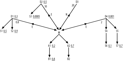
Fill in the missing ratios for the correlated joins. Assume that
t=5 (the rowcount of the whole query, including the
NOT EXISTS subquery), while
q=50 (the rowcount of the query with the NOT EXISTS condition removed). Find the best
join order, including all the tables in the subqueries and in the outer
query.