
7
Satellite Link Design Fundamentals
In this chapter, as the title of the chapter itself suggests, a comprehensive look will be taken at the important parameters that govern the design of a satellite communication link. The significance of each one of these parameters will be discussed vis-à-vis the overall link performance in terms of both quantity and quality of services provided by the link, without of course losing sight of the system complexity of both the Earth station and the space segment and the associated costs involved therein. What is implied by the previous sentence is that for a given link performance, a better system performance could perhaps be provided by making the Earth station and spacecraft instrumentation more complex, thereby increasing overall costs, sometimes to the extent of making it an unviable proposition.
The designer must therefore attempt to optimize the overall link, giving due attention to each element of the link and the factors associated with its performance. The chapter begins with a brief introduction to various parameters that characterize a satellite link or influence its design. Each one of these parameters is then dealt with in greater detail. This is followed by the basics of link design and the associated mathematical treatment, which is suitably illustrated with a large number of illustrations and design examples.
7.1 Transmission Equation
The transmission equation relates the received power level at the destination, which could be the Earth station or the satellite in the case of a satellite communication link, to the transmitted RF power, the operating frequency and the transmitter–receiver distance. It is fundamental to the design of not only a satellite communication link but also any radio communication link because the quality of the information delivered to the destination is governed by the level of the signal power received. The reason for this is that it is the received carrier-to-noise ratio that is going to decide the quality of information delivered, and for a given noise contribution from various sources, both internal and external to the system, the level of received power is vital to the design of the communication link. An estimation of received power level in a satellite communication link is made in the following paragraphs.
It is assumed that the transmitter radiates a power PT watts with an antenna having a gain GT as compared to the isotropic radiation level. The power flux density (PRD in W/m2) due to the radiated power in the direction of the antenna bore sight at a distance d metres is given by
The product PTGT is the effective isotropic radiated power (EIRP). Also, if the radiating aperture AT of the transmitting antenna is large as compared to λ2, where λ is the operating wavelength, then GT equals (4πAT/λ2). If AR is the aperture of the receiving antenna, then the received power PR at the receiver at a distance d from the transmitter can be expressed as
where AR is related to the receiver antenna gain by GR = 4πAR/λ2. The expression for the received power is modified to
or
The term (4πd/λ)2 represents the free space path loss LP. The above expression is also known as the Friis transmission equation. The received power can be expressed in decibels as
The above equation can be modified to include other losses, if any, such as losses due to atmospheric attenuation, antenna losses, etc. For example, if LA, LTX and LRX are the losses due to atmospheric attenuation, transmitting antenna and receiving antenna respectively, then the above equation can be rewritten as
7.2 Satellite Link Parameters
Important parameters that influence the design of a satellite communication link include the following:
- Choice of operating frequency
- Propagation considerations
- Noise considerations
- Interference-related problems
7.2.1 Choice of Operating Frequency
The choice of frequency band from those allocated by the International Telecommunications Union (ITU) for satellite communication services such as the fixed satellite service (FSS), the broadcast satellite service (BSS) and the mobile satellite service (MSS) is mostly governed by factors like propagation considerations, coexistence with other services, interference-related issues, technology status, economic considerations and so on. While it may be more economic to use lower frequency bands, there would be interference-related problems as a large number of terrestrial microwave links use frequencies within these bands. Also, lower frequency bands would offer lower bandwidths and hence a reduced transmission capacity. Higher frequency bands offer higher bandwidths but suffer from the disadvantage of severe rain-induced attenuation, particularly above 10 GHz. Also, above 10 GHz, rain can have the effect of reducing isolation between orthogonally polarized signals in a frequency re-use system. It may be mentioned here that for frequencies less than 10 GHz and elevation angles greater than 5°, atmospheric attenuation is more or less insignificant.
7.2.2 Propagation Considerations
The nature of propagation of electromagnetic waves or signals through the atmospheric portion of an Earth station–satellite link has a significant bearing on the link design. From the viewpoint of a transmitted or received signal, it is mainly the operating frequency and to a lesser extent the polarization that would decide how severe the effect of atmosphere is going to be. From the viewpoint of atmosphere, it is the first few tens of kilometres constituting the troposphere and then the ionosphere extending from about 80 km to 1000 km that do the damage. The effect of atmosphere on the signal is mainly in the form of attenuation caused by atmospheric scattering and scintillation and depolarization caused by rain in the troposphere and Faraday rotation in the ionosphere. While rain-induced attenuation is very severe for frequencies above 10 GHz, polarization changes due to Faraday rotation are severe at lower frequencies and are almost insignificant beyond 10 GHz. In fact, atmospheric attenuation is the least in the 3 to 10 GHz window. That is why it is the preferred and most widely used one for satellite communications.
7.2.3 Noise Considerations
In both analogue and digital satellite communication systems, the quality of signal received at the Earth station is strongly dependent on the carrier-to-noise ratio of the satellite link. The satellite link comprises an uplink, the satellite channel and a downlink. The quality of the signal received on the uplink therefore depends upon how strong the signal is, as it leaves the originating Earth station and how the satellite receives it. On the downlink, it depends upon how strongly the satellite can retransmit the signal and then how the destination Earth station receives it. Because of the large distances involved, the signals received by the satellite over the uplink and received by the Earth station over the downlink are very weak. Satellite communication systems, moreso the geostationary satellite communication systems are therefore particularly susceptible to noise because of their inherent low received power levels. In fact, neither the absolute value of the signal nor that of the noise should be seen in isolation for gauging the effectiveness of the satellite communication link. If the received signal is sufficiently weak as compared to the noise level, it may become impossible to detect the signal. Even if the signal is detectable, steps should be taken within the system to reduce the noise to an acceptable level lest it impairs the quality of the signal received.
The sources of noise include natural and man-made sources, as well as the noise generated in the Earth station and satellite equipment. While the man-made noise mainly arises from electrical equipment and is almost insignificant above 1 GHz, the natural sources of noise include solar radiation, sky noise, background noise contributed by Earth, galactic noise due to electromagnetic waves emanating from radio stars in the galaxy and the atmospheric noise caused by lightening flashes and absorption by oxygen and water vapour molecules followed by re-emission of radiation. Sky noise and solar noise can be avoided by proper orientation and directionality of antennas. Galactic noise is insignificant above 1 GHz. Noise due to lightning flashes is also negligible at satellite frequencies.
7.2.4 Interference-related Problems
Major sources of interference include interference between satellite links and terrestrial microwave links sharing the same operational frequency band, interference between two satellites sharing the same frequency band, interference between two Earth stations accessing different satellites operating in the same frequency band, interference arising out of cross-polarization in frequency re-use systems, adjacent channel interference inherent to FDMA systems and interference due to intermodulation phenomenon.
Interference between satellite links and terrestrial links could further be of two types: first where terrestrial link transmission interferes with reception at an Earth station and the second where transmission from an Earth station interferes with terrestrial link reception. The level of inter-satellite and inter-Earth station interference is mainly governed by factors like the pointing accuracy of antennas, the width of transmit and receive beams, intersatellite spacing in the orbit of two co-located satellites, and so on. Cross-polarization interference is caused by coupling of energy from one polarization state to another polarization state when a frequency re-use system employs orthogonal linear polarizations (horizontal and vertical polarization) or orthogonal circular polarization (left-hand and right-hand circular polarization). This coupling of energy occurs due to a finite value of cross-polarization discrimination of the Earth station and satellite antennas and also to depolarization caused by rain. Adjacent channel interference arises out of overlapping amplitude characteristics of channel filters. Intermodulation interference is caused by the intermodulation products produced in the satellite transponder when multiple carriers are amplified in the high power amplifier that has both amplitude as well as phase nonlinearity.
7.3 Frequency Considerations
The choice of operating frequency for a satellite communication service is mainly governed by factors like propagation considerations, coexistence with other services, noise considerations and interference-related issues. These have been briefly discussed in the preceding paragraphs and will be dealt with at length in the sections to follow. The requirement for co-existence with other services and the fact that there will always be competition to use the optimum frequency band by various agencies with an eye to getting the best link performance show that there is always a need for a mechanism for allocation and coordination of the frequency spectrum at the international level. A brief on frequency allocation and the coordination mechanism is given in the following paragraphs.
7.3.1 Frequency Allocation and Coordination
Satellite communication employs electromagnetic waves for transmission of information between Earth and space. The bands of interest for satellite communications lie above 100 MHz and include the VHF, UHF, L, S, C, X, Ku and Ka bands. (Various microwave frequency bands are listed in Table 7.1). Higher frequencies are employed for satellite communication, as the frequencies below 100 MHz are either reflected by the ionosphere or they suffer varying degrees of bending from their original paths due to refraction by the ionosphere. Initially, the satellite communication was mainly concentrated in the C band (6/4 GHz) as it offered fewest propagation as well as attenuation problems. However, due to overcrowding in the C band and the advances made in the field of satellite technology, which enabled it to deal with the propagation problems in the higher frequency bands, newer bands like the X, Ku and Ka bands are now being employed for commercial as well as military satellite applications. Moreover, use of these higher frequencies gives satellites an edge over terrestrial networks in terms of the bandwidth offered by a satellite communication system.
Table 7.1 Microwave frequency bands for satellite communication.
| Band | Frequency (GHz) |
| L band | 1–2 |
| S band | 2–4 |
| C band | 4–8 |
| X band | 8–12 |
| Ku band | 12–18 |
| K band | 18–27 |
| Ka band | 27–40 |
| V band | 40–75 |
| W band | 75–110 |
As the frequency spectrum is limited, it is evident the frequency bands are allocated in such a manner as to ensure their rational and efficient use. The International Telecommunication Union (ITU), formed in the year 1865, is a specialized institution that ensures the proper allocation of frequency bands as well as the orbital positions of the satellite in the GEO orbit. ITU carries out these regulatory activities through its four permanent organs, namely the General Secretariat, the International Frequency Registration Board (IFRB), the International Radio Consultative Committee (CCIR) and the International Telegraph and Telephone Consultative Committee (CCITT). The ITU organizes the international radio conferences such as World Administrative Radio Conferences (WARC) and other regional conferences to issue guidelines for frequency allocation for various services. These allocations are made either on an exclusive or shared basis and can be put into effect worldwide or limited to a region. The frequency bands that are allocated internationally are in turn reallocated by the national government bodies of the individual countries. Each country is assigned frequencies according to its requirements. The main purpose is to ensure that the technical parameters are retained for a period of at least 10 to 20 years and to guarantee that all countries can access the satellite service when needed. The ITU has divided the frequency allocations for different services into various categories: primary, secondary, planned, shared, etc. In primary frequency allocation, a service has an exclusive right of operation. In secondary frequency allocation, a service is not guaranteed interference protection and neither is it permitted to cause interference to services with primary status. WARC divided the globe into three regions for the purpose of frequency allocations.
They are:
- Region 1. Including Europe, Africa, USSR and Mongolia
- Region 2. Including North and South America, Hawaii and Greenland
- Region 3. Including Australia, New Zealand and those parts of Asia and the Pacific not included in regions 1 and 2.
It has also classified the various satellite services into the following categories, including fixed satellite services (FSS), intersatellite links (ISL), mobile satellite services (MSS), broadcasting satellite services (BSS). Earth exploration services, space research activities, meteorological activities, space operation, amateur radio services, radio determination, radio navigation, aeronautical radio navigation and maritime radio navigation. Among these applications the FSS, MSS and BSS are the principle communication-related applications of satellites.
The fixed satellite service (FSS) refers to the two-way communication between two Earth stations at fixed locations via a satellite. It supports the majority of commercial applications including satellite telephony, satellite television and data transmission services. The FSS primarily uses two frequency bands: the C band (6/4 GHz), which provides lower power transmission over a wide geographic area requiring large antennas for reception, and the Ku band (14/11 GHz, 14/12 GHz), which offers higher transmission power over a smaller geographical area, enabling reception by small receiving antennas. All of the C band and much of the Ku band have been allocated for international and domestic FSS applications. The X band (8/7 GHz) is used to provide fixed services to government and military users. EHF (extremely high frequency), UHF (ultra high frequency) and SHF (super high frequency) band transponders are also used in military satellites.
The broadcast satellite service (BSS) refers to the satellite services that can be received at many unspecified locations by relatively simple receive-only Earth stations. These Earth stations can either be community Earth stations serving various distribution networks or located in homes for direct-to-home transmission. The Ku band (18/12 GHz) and the Ka band (30/20 GHz) are mainly used for BSS applications, like television broadcasting and DTH applications.
The mobile satellite service (MSS) refers to the reception by receivers that are in motion, like ships, cars, lorries, and so on. It comprises land mobile services, maritime mobile services and aeronautical mobile services. Increasingly, MSS networks are providing relay communication services to portable handheld terminals. The L band (2/1 GHz) and the S Band (4/2.5 GHz) are mainly employed for MSS services because, at these lower microwave frequencies, broader beams are transmitted from the satellite, enabling the reception by antennas even if they are not pointed towards the satellite. This in turn makes these frequencies attractive for mobile and personal communications. The lower frequencies in the VHF and UHF bands are mainly employed for messaging and positioning applications, as these applications require smaller bandwidths. Some LEO satellite constellations are using these frequencies to provide the above-mentioned applications. Table 7.2 enumerates a partial list of frequency allocations for satellite communications and the satellites using them.
Table 7.2 Frequency allocations for satellite communication.
| Frequency band | Satellite service | Examples |
| VHF (<200 MHz) | Messaging | Starsys constellation of 24 satellites in the LEO orbit, having an uplink frequency of 148–150 MHz and a downlink frequency of 137–138 MHz |
| UHF (200 MHz–1 GHz) | Messaging and positioning, voice and fax | Gonets is a Russian messaging satellite constellation comprising 18 satellites in the LEO. Uplink frequencies are 312–315 MHz and 1624.5–1643.4 MHz and downlink frequencies are 387–390 MHz and 1523–1541.9 MHz |
| L band (2/1 GHz) | MSS and positioning | Inmarsat-II satellite having 4 L band transponders supporting mobile-to-mobile services with an uplink frequency of 1.6 GHz and a downlink frequency of 1.5 GHz |
| S band (4/2.5 GHz) | MSS | NStar-C satellite having 20 S band transponders provides S band mobile communication services to Japan |
| C band Uplink 5.925–6.425 GHz Downlink 3.7–4.2 GHz | FSS | Palapa-B, Indonesia's domestic satellite comprises 20 C band transponders each capable of carrying 1000 two-way voice circuits or a colour television transmission channel. It has uplink frequencies of 5.925–6.425 GHz and downlink frequencies of 3.7–4.2 GHz |
| X band Uplink 7.9–8.4 GHz Downlink 7.25–7.75 GHz | Military applications | Hispasat-1B satellite operated by the Spanish government carries four X band transponders for military applications |
| Ku band Europe | FSS, BSSand Telecom | Hot Bird-6 satellite consists of 28Ku band transponders, whichprovide television broadcast andmultimedia services over theentire European continent, NorthAfrica and the Middle East |
| FSS | ||
| Uplink 14–14.8 GHz | ||
| Downlink 10.7–11.7 GHz | ||
| BSS | ||
| Uplink 17.3–18.1 GHz | ||
| Downlink 11.7–12.5 GHz | ||
| Telecom | ||
| Uplink 14–14.8 GHz | ||
| Downlink 12.2–12.75 GHz | ||
| USA | ||
| FSS | ||
| Uplink 14–14.5 GHz | ||
| Downlink 11.7–12.2 GHz | ||
| BSS | ||
| Uplink 17.3–17.8 GHz | ||
| Downlink 12.2–12.7 GHz | ||
| Ka band | FSS, BSS | Superbird-6 satellite, having 23 Kuand 6 Ka band transponders, provides business communicationservices to Japan in Ku and Kabands and additional Ka bandservices using a steerable spot beam |
| FSS | ||
| Uplink 27–31 GHz | ||
| Downlink 17–21 GHz | ||
Current trends in satellite communication indicate the opening of new higher frequency bands for various applications, like the Q band (33–46 GHz) and the V band (46–56 GHz), which are being considered for use in FSS, BSS and intersatellite communication applications. Another important concept is the sharing of the same frequency bands between GEO and new systems for personal satellite communications using non-GEO orbits.
When an organization intends to add a new satellite system, frequencies close to those used in the existing system are preferred in order to minimize the impact of the planned expansion on the existing customers and also changes to the space segment. For many applications like the DTH service, frequency and other parameter considerations have already been assigned by the ITU for each country. In these cases the new frequency assignment becomes easy and straight forward. When such a frequency plan does not exist, the system designer selects frequencies from the ITU allocations based on the trade-off analysis taking into account the technical (propagation, state of the technology) and economic factors. A notification is sent to the ITU about the details of the new system (planned satellite location). After selecting the frequency band, the next step is to resolve all the interference related problems that might occur by coordinating with all the system operators. After resolving all the issues with other operators, ITU is again notified and the ITU enters the allocations in its frequency register. The new system is then considered operational.
7.4 Propagation Considerations
As outlined earlier, the nature of propagation of electromagnetic waves through the atmosphere has a significant bearing on the satellite link design. As will be seen in the paragraphs to follow, it is the first few tens of kilometres constituting the troposphere and then the ionosphere extending from about 80 km to 1000 km that do the major damage.
The effect of the atmosphere on the signal is mainly in the form of atmospheric gaseous absorption, cloud attenuation, topospheric scintillation causing refraction, Faraday rotation in the ionosphere, ionospheric scintillation, rain attenuation and depolarization. Both attenuation and depolarization come from interactions between the propagating electromagnetic waves and different sections of the atmosphere.
Attenuation is defined as the difference between the power that would have been received under ideal conditions and the actual power received at a given time.
Where,
- A(t) is the attenuation at any given time t
- Prideal(t) is the received power under ideal conditions at time t
- Practual(t) is the actual received power at time t
Depolarization refers to the conversion of energy from the wanted channel to the unwanted channel. Here, wanted channel refers to the co-polarized channel and the unwanted channel refers to the cross-polarized channel. Due to de-polarization, co-channel interference and cross-talk occurs between dual-polarized satellite links.
Propagation losses are further of two types, namely those that are more or less constant and therefore predictable and those that are random in nature and therefore unpredictable. While free-space loss belongs to the first category, attenuation caused due to rain is unpredictable to a large extent. The second category of losses can only be estimated statistically. The combined effect of these two types of propagation losses is to reduce the received signal strength. Due to the random nature of some types of losses, the received signal strength fluctuates with time and may even reduce to a level below the minimum acceptable limit for as long a period as an hour in 24 hours during the period of severe fading. This is amply illustrated in the graph of Figure 7.1.
Figure 7.1 Fading phenomenon
7.4.1 Free-space Loss
Free-space loss is the loss of signal strength only due to distance from the transmitter. While free space is a theoretical concept of space devoid of all matter, in the present context it implies remoteness from all material objects or forms of matter that could influence propagation of electromagnetic waves. In the absence of any material source of attenuation of electromagnetic signals, therefore, the radiated electromagnetic power diminishes as the inverse square of the distance from the transmitter, which implies that the power received by an antenna of 1 m2 cross-section will be Pt/(4πR2) where Pt is the transmitted power and R is the distance of the receiving antenna from the transmitter. In the case of uplink, the Earth station antenna becomes the transmitter and the satellite transponder is the receiver. It is the opposite in the case of downlink.
The free-space path loss component can be computed from
where LFS is the free space loss and λ = operating wavelength. Also, λ = c/f, where
- c = velocity of electromagnetic waves in free space
- f = operating frequency
- If c is taken in km/s and f in MHz, then the free-space path loss can also be computed from
7.4.2 Gaseous Absorption
Electromagnetic energy gets absorbed and converted into heat due to gaseous absorption as it passes through the troposphere. The absorption is primarily due to the presence of molecular oxygen and uncondensed water vapour and has been observed to be not so significant as to cause problems in the frequency range of 1 to 15 GHz. Of the other gases, atmospheric nitrogen does not have a peak while carbon dioxide has shown a peak at around 300 GHz. The presence of free electrons in the atmosphere also causes absorption due to collision of electromagnetic waves with these electrons. However, electron absorption is significant only at frequencies less than 500 MHz. Figure 7.2 shows the plot of total absorption (in dB) towards the zenith, that is for an elevation angle of 90° as a function of frequency. It can be seen from this plot that there are specific frequency bands where the absorption is maximum, near total. The first absorption band is caused due to the resonance phenomenon in water vapour and occurs at 22.2 GHz. The second band is caused by a similar phenomenon in oxygen and occurs around 60 GHz. These bands are therefore not employed for either uplinks or downlinks. However, they can be used for intersatellite links. It should also be mentioned that absorption at any frequency is a function of temperature, pressure, relative humidity (RH) and elevation angle.
Figure 7.2 Gaseous absorption as a function of frequency and elevation angle
Absorption increases with a decrease in elevation angle E due to an increase in the transmission path. Absorption at any elevation angle E less than 90° can be computed by multiplying the absorption figure for 90° degree elevation by 1/sin E. Applying this correction, it is observed that the one-way absorption figure range in the 1–15 GHz frequency band increases from (0.03–0.2 dB) for 90° elevation to (0.35–2.3 dB) for 5° elevation. Absorption is also observed to increase with humidity. In the case of resonance absorption of water vapours around 22.2 GHz, it varies from as low as 0.05 dB (at 0 % RH) to about 1.8 dB (at 100 % RH). It may also be mentioned here that the data given in Figure 7.2 applies to the Earth station at sea level and the losses would reduce with an increase in height of the Earth station.
It is evident from the plots of Figure 7.2 that there are two transmission windows in which absorption is either insignificant or has a local minimum. The first window is in the frequency range of 500 MHz to 10 GHz and the second is around 30 GHz. This explains the wide use of the 6/4 GHz band. The increasing interest in the 30/20 GHz band is due to the second window, which shows a local minimum around 30 GHz. Losses at the 14/11 GHz satellite band are within acceptable limits with values of about 0.8 dB for 5° elevation and 0.2 dB for 15° elevation.
7.4.3 Attenuation due to Rain
After the free-space path loss, rain is the next major factor contributing to loss of electromagnetic energy caused by absorption and scattering of electromagnetic energy by rain drops. It may be mentioned here that the loss of electromagnetic energy due to gaseous absorption discussed in the earlier paragraphs tends to remain reasonably constant and predictable. On the other hand, the losses due to precipitation in the form of rain, fog, clouds, snow, and so on, are variable and far less predictable. However, losses can be estimated in order to allow the satellite links to be designed with an adequate link margin wherever necessary.
Losses due to rain increases with an increase in frequency and reduction in the elevation angle. Figure 7.3 shows rain attenuation in dB as a function of frequency for a set of different elevation angles. It is evident from the family of curves that there is not much to worry about from rain attenuation for C band satellite links. Attenuation becomes significant above 10 GHz and therefore when a satellite link is planned to operate beyond 10 GHz, an estimate of rain-caused attenuation is made by making extensive measurements at several locations in the coverage area of the satellite system.

Figure 7.3 Rain-caused attenuation as a function of frequency and elevation angle
Attenuation of electromagnetic waves due to rain (Arain) extended over a path length of L can be computed from
where α = specific attenuation of rain in dB/km. Specific attenuation again depends upon various factors like rain drop size, drop size distribution, operating wavelength and the refractive index. In practice, rain attenuation is estimated from
where a and b are frequency and temperature-dependent constants and R is the surface rain rate at the location of interest.
In addition to attenuation of electromagnetic energy, another detrimental effect caused by rain is depolarization. This reduces the cross-polarization isolation. This effect has been observed to be more severe on circularly polarized waves than linearly polarized waves. Depolarization of electromagnetic waves due to rain is caused by flattening of supposedly spherical rain drops affected by atmospheric drag. Depolarization is not particularly harmful at the C band and lower parts of the Ku band. It is severe at frequencies beyond 15 GHz.
7.4.4 Cloud Attenuation
Attenuation due to clouds is more or less irrelevant for lower frequency bands (L, S, C and Ku bands), but is largely relevant for satellite systems employing Ka and V band frequencies. The attenuation figure for water-filled clouds is much larger than the attenuation figure for clouds made from ice crystals. It may be mentioned here that the attenuation figure for ice clouds is negligible for the frequency bands of interest. The typical figure of attenuation for water filled clouds is of the order of 1 to 3 dB for frequency bands around 30 GHz at elevation angle of 30° in temperate latitude locations. However, the attenuation figures increase with increase in the thickness of the clouds and its probability of occurrence. In addition, the cloud attenuation increases for lower elevation angles.
7.4.5 Signal Fading due to Refraction
Refraction is the phenomenon of bending of electromagnetic waves as they pass through the different layers of the atmosphere. Refraction of the satellite beams occur in the troposphere (lower layer of the atmosphere from the Earth's surface to a height of 15 km approximately) due to the variations in the refractive index of the air column. The variations in the refractive index is the result of the turbulent mixing of the different columns of the air due to the agitative convective activity in the troposphere caused by heating of the Earth's surface by the sun. The variations in the refractive index lead to bending of electromagnetic waves resulting in fluctuations in the received signal levels, also referred to as scintillations. The result of bending of electromagnetic waves is depicted in Figure 7.4. It leads to a virtual position for the satellite slightly above the true position of the satellite. The random nature of bending due to discontinuities and fluctuations caused by unstable atmospheric conditions like temperature inversions, clouds and fog produces signal fading, which leads to loss of signal strength. Fading is the phenomenon wherein the Earth station receiving antenna receives the signal transmitted by the satellite via different paths with different phase shifts. The fading phenomenon is more adverse at lower elevation angles.

Figure 7.4 Bending of electromagnetic waves caused by refraction in the atmosphere
It may be mentioned here that the topospheric scintillation does not cause depolarization. The scintillation effects increase for higher frequencies, lower path elevation angles and for warmer and humid climate. The effect is more severe for terrestrial links and not too worrisome for satellite links, as the amount of bending caused in a satellite link is small relative to the beam width of the satellite and Earth station antennas.
7.4.6 Ionosphere-related Effects
The ionosphere is an ionized region in space, extending from about 80–90 km to 1000 km (Figure 7.5) formed by interaction of solar radiation with different constituent gases of the atmosphere. Electromagnetic waves travelling through the ionosphere are affected in more than one way, some more predominant than the other from the viewpoint of satellite communications. The effects that are of concern and need attention include polarization rotation, also called the Faraday effect, and scintillation, which is simply rapid fluctuation of the signal amplitude, phase, polarization or angle of arrival. The ionosphere also affects the propagating electromagnetic waves in many other ways, such as absorption, causing propagation delay, dispersion, etc. However, these effects are negligible at the frequencies of main interest for satellite communications, except for very small time periods during intense solar activity such as solar flares. Also, most ionospheric effects including those of primary interest, like polarization rotation and scintillation, decrease with an increase in frequency having a 1/f2 dependence. The two major effects are briefly described in the following paragraphs.
Figure 7.5 Different layers of atmosphere
7.4.6.1 Polarization Rotation – Faraday Effect
When an electromagnetic wave passes through a region of high electron content like the ionosphere, the plane of polarization of the wave gets rotated due to interaction of the electromagnetic wave with the Earth's magnetic field. The angle through which the plane of polarization rotates is directly proportional to the total electron content of the ionized region and inversely proportional to the square of the operating frequency. It also depends upon the state of the ionosphere, time of the day, solar activity, the direction of the incident wave, and so on. Directions of polarization rotation are opposite for transmit and receive signals.
Due to its 1/f2 dependence, the effect is observed to be pronounced only at frequencies below 2 GHz. The worst case polarization rotation angle may be as large as 150° in certain conditions at 1 GHz. Applying 1/f2 dependence, the rotation angle may be as small as 9° at 4 GHz and 4° at 6 GHz. It would reduce to a fraction of a degree in the Ku band frequency range. Except for a small time period during unusual atmospheric conditions caused by intense solar activity, magnetic storms, and so on, the Faraday effect is more or less predictable and therefore can be compensated for by adjusting the polarization of the receiving antenna. Circular polarization is virtually unaffected by Faraday effect and therefore its impact can be minimized by using circular polarization.
The polarization rotation angle (ΔΨ) for a path length through the ionosphere of Z metres is given by
Where,
- ΔΨ is the rotation angle (radians)
- θ is the angle between the geomagnetic field and the direction of propagation of the wave
- N is the electron density (electrons/cm3)
- Bo is the geomagnetic flux density (Tesla)
- f is the operating frequency (Hz)
For a polarization rotation angle (also referred to as the polarization mismatch angle) of ΔΨ, the attenuation of the co-polar signal given by
where, APR is the attenuation due to polarization rotation in dB.
The mismatch also produces a cross-polarized component, which reduces the cross-polarization discrimination (XPD), given by
where, XPD is the cross-polarization discrimination in dB.
The magnitudes of attenuation and XPD due to polarization mismatch will be 0.1 dB and 16 dB respectively at 4 GHz for which ΔΨ = 9°.
7.4.6.2 Ionospheric Scintillation
As mentioned above, scintillation is nothing but the rapid fluctuations of the signal amplitude, phase, polarization or angle-of-arrival. In the ionosphere, scintillation occurs due to small scale refractive index variations caused by local electron concentration fluctuations. The total electron concentration (total number of electrons existing in a vertical column of 1m2 area) of the ionosphere increases by two orders of magnitude during the day as compared to night due to the energy received from the sun. This rapid change in the value of total electron concentration from the daytime value to the nighttime value gives rise to irregularities in the ionosphere. It mainly occurs in the F-region of the ionosphere due to the highest electron concentration in that region.
The irregularities cause refraction resulting in rapid variations in the signal amplitude and phase, which leads to rapid signal fluctuations that are referred to as ionospheric scintillations. As a result, the signal reaches the receiving antenna via two paths, the direct path and the refracted path, as illustrated in Figure 7.6. Multipath signals can lead to both signal enhancement as well as signal cancellation depending upon the phase relationship with which they arrive at the receiving antenna. The resultant signal is a vector addition of the direct and the refracted signal. In the extreme case, when the strength of the refracted signal is comparable to that of the direct signal, cancellation can occur when the relative phase difference between the two is 180°. On the other hand, an instantaneous recombination of the two signals in phase can lead to signal amplification up to 6 dB.
Figure 7.6 Ionospheric scintillation
The scintillation effect is inversely proportional to the square of the operating frequency and is predominant at lower microwave frequencies, typically below 4 GHz. Scintillation, however, increases during periods of high solar activity and other extreme conditions such as the occurrence of magnetic storms. Scintillation has also been observed to be maximum in the region that is ±25° around the equator. Under such adverse conditions, scintillation can cause problems at 6/4 GHz band too. At the Ku band and beyond, however, the effect is negligible. Also, unlike scintillation caused by the troposphere, ionospheric scintillation is independent of the elevation angle.
In regions where scintillation is expected to cause problems, an adequate link margin in the form of additional transmitted power should be catered for to take care of the effect and maintain link reliability.
7.4.7 Fading due to Multipath Signals
Ionospheric scintillation, as illustrated above, results in a multipath phenomenon where the indirect signal is produced as a result of refraction caused by pockets of ion concentration in the F-region of the ionosphere. Multipath signals also result from reflection and scattering from obstacles such as buildings, trees, hills and other man-made and natural objects. In the case of fixed satellite terminals, the situation remains more or less the same and does not change with time as long as the satellite remains in the same position with respect to the satellite terminal (Figure 7.7). However, in the case of mobile satellite terminals, the situation keeps changing with time. In a typical case, a mobile terminal could receive the direct signal and another signal reflected off the highway, buildings, neighbouring hills or trees. The relative phase difference between the two signals could produce either a signal enhancement or fading (Figure 7.8). Moreover, the fading signal varies with time as the satellite moves with respect to the points of reflection.
Figure 7.7 Fading due to multipath signals for a fixed satellite terminal
Figure 7.8 Mobile satellite terminal receiving multipath signals
Thus, the situation in the case of mobile satellite service (MSS) terminals is far more severe and uncertain than it is in the case of fixed receiving terminals. The mobile station–satellite path profile keeps changing continuously with the movement of the mobile terminal. Also, mobile terminals usually employ broadband receiving antennas, which do not provide adequate discrimination against signals received via indirect paths.
7.5 Techniques to Counter Propagation Effects
As mentioned before, the propagation effects can be broadly classified as attenuation effects and depolarization effects. The attenuation effects can be countered by employing the following techniques:
- Power Control
- Signal Processing
- Diversity
The depolarization effects can be negated by employing depolarization compensation. In this section all of these techniques are briefly explained.
7.5.1 Attenuation Compensation Techniques
The attenuation compensation techniques are described in the following paragraphs.
- Power Control: Power control refers to varying the EIRP of the signal to enhance the C/N ratio. Adaptive power control is applied wherein the transmitter power is adjusted to compensate for the changes in the signal attenuation along the transmission path. This is referred to as up-link power control (ULPC) and it results in enhancement of the overall availability of the connection. ULPC can be done either in open-loop mode or in closed loop mode. In the open-loop mode, the fade level on the downlink signal is used to predict the likely fade level occurring on the uplink signal and accordingly the signal power is increased. In the closed-loop mode, the signal power is detected at the satellite and it sends a control signal to the Earth station to adjust the transmitted power in accordance with the attenuation in real-time. As is evident, closed loop control is more accurate that the open loop control. However, it is more expensive than open loop control.
- Signal Processing: Signal processing refers to onboard processing techniques on the satellite to translate the signals coming from the Earth station via the uplink to baseband levels for processing and onward transmission back to the Earth. The satellite transponder demodulates the incoming up-link signal from the Earth station, demultiplexes it and decodes it. Each traffic packet is handled at the baseband level and therefore most of the bit errors can be removed. In addition, the signal level of each packet is detected and the transmitting Earth station is alerted in case the energy level of the received packet has fallen beyond a certain threshold. The packets are then coded, multiplexed and modulated for retransmission back to the Earth.
- Diversity: Many diversity schemes exist that can be used to enhance the signal levels but are not implemented due to the costs involved. Diversity schemes include time diversity, frequency diversity and site diversity. Site diversity scheme is most potential candidate to be employed as it offers the maximum gain. In time diversity, additional slots are assigned to the rain-affected link in the TDMA frame so that the same signal can be sent at a smaller bit rate, thereby reducing the bandwidth and increasing the C/N ratio. In frequency diversity, the frequency band of the signal is changed from the band having large attenuation to the band having less attenuation. As an example, a rain affected Ku band link can be switched to a C band which is not attenuated significantly by rain. This requires additional C band transmitting capability and the receiving capability at the transmitter and receiver Earth stations respectively. Site diversity is a technique wherein two or more Earth stations are located sufficiently apart so that the rain and other attenuation impairments observed by signals from each of the Earth stations to the satellite are not correlated. The Earth stations are connected to each other so that any Earth station can be used to support the traffic from other Earth station/s suffering from attenuation.
7.5.2 Depolarization Compensation Techniques
Depolarization compensation is a technique used to compensate for the depolarization effects caused to the signal during its propagation through the atmosphere. Here the feed system of the antenna is adjusted in such a way to correct for depolarization in the path. Another compensation technique is to cross-couple the orthogonal channels at the receiver and determine the depolarized signal. The depolarized signal is then removed by subtracting it from the received signal. Only a few Earth stations have implemented depolarization compensation as it is an expensive proposition.
7.6 Noise Considerations
Satellite communication systems are particularly susceptible to noise because of their inherent low received power levels, as the signals received by the satellite over the uplink and received by the Earth station over the downlink are very weak due to involvement of large distances. Sources of noise include natural and man-made sources and also the noise generated inside the Earth station and satellite equipment, as outlined during the introductory paragraphs at the beginning of the chapter. From the viewpoint of satellite communications, the natural and man-made sources of noise can either be taken care of or are negligible. It is mainly the noise generated in the equipment where attention primarily needs to be paid. In the paragraphs to follow, various parameters that can be used to describe the noise performance of various building blocks individually and also as a system, which is a cascaded arrangement of those building blocks, will be briefly discussed.
7.6.1 Thermal Noise
Thermal noise is generated in any resistor or resistive component of any impedance due to random motion of molecules, atoms and electrons. It is called thermal noise as the temperature of a body is the statistical RMS value of the velocity of motion of these particles. It is also called ‘white’ noise because, due to randomness of the motion of particles, the noise power is evenly spread over the entire frequency spectrum. It is also known as Johnson noise.
According to kinetic theory, the motion of these particles ceases at absolute zero temperature, that is zero degrees kelvin. Therefore, the noise power generated in a resistor or resistive component is directly proportional to its absolute temperature, in addition to the bandwidth over which it is measured; that is
where
- T = absolute temperature(in K)
- B = bandwidth of interest(in Hz)
- k = Boltzmann' s constant = 1.38 × 10⁻²³ J/K
- Pn = noise power output of a resistor(in W)
Thermal noise power at room temperature (T = 290 K) in dBm (decibels relative to a power level of 1mW) can also be computed from
If the resistor is considered as a noise generator with an equivalent noise voltage equal to Vn, then this noise generator will transfer maximum noise power Pn to a matched load that is given by
which gives expression for noise voltage (Vn) as
Expression for noise current (In) can be deduced from the expression for noise voltage and is given by
Another term that is usually defined in this context is the noise power spectral density given by
where, Pno is the noise power spectral density in W/Hz.
This implies that the noise power spectral density increases with physical temperature of the device. Also, thermal noise generated in a device can be reduced by reducing its physical temperature or the bandwidth over which the noise is measured or both.
7.6.2 Noise Figure
The noise figure F of a device can be defined as the ratio of the signal-to-noise power at its input to the signal-to-noise power at its output; i.e.
where
- Si = available signal power at the input
- Ni = available noise power at the input
- So = available signal power at the output
- No = available noise power at the output(in a noiseless device)
- G = power gain over the specified bandwidth = So/Si
Now, Ni = kTiB, where Ti is the ambient temperature in kelvin. Therefore, the noise figure (F) is expressed as
The actual amplifier, however, introduces some noise, which is added to the output noise power. If the noise power introduced is ΔN, then
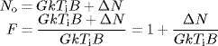
The noise figure is thus the ratio of the actual output noise to that which would remain if the device itself did not introduce any noise. In the case of a noiseless device, ΔN = 0, which gives F = 1. Thus the noise figure in the case of an ideal device is unity. Any value of the noise figure greater than unity means a noisy device.
7.6.3 Noise Temperature
Yet another way of expressing noise performance of a device is in terms of its equivalent noise temperature Te. It is the temperature of a resistance that would generate the same noise power at the output of an ideal (i.e. noiseless) device as that produced at the output by an actual device when terminated at its input by a noiseless resistance, i.e. a resistance at absolute zero temperature.
Now, noise generated by the device ΔN = GkTeB, which when substituted in the expression for noise figure mentioned above gives
In the preceding paragraphs, noise figure and noise temperature specifications of devices have been discussed and a relationship between the two parameters commonly used for measuring a device's noise performance has been established. It will now be shown how the expression for the effective noise temperature is modified in the case where the device is purely a resistive attenuator with a specified attenuation or loss factor.
If L is the loss factor, then the gain G for this attenuator can be expressed as G = 1/L. The expression for the total noise power at the output of the attenuator (No) can be written as
where Te = effective noise temperature of the attenuator. If the attenuator is considered to be at the same temperature (Ti) as that of the source resistance from which it is fed, then the value of output noise (No) is given by
This gives
or
This expression gives the effective noise temperature of a noise source at temperature Ti, followed by a resistive attenuator having a loss factor L.
7.6.4 Noise Figure and Noise Temperature of Cascaded Stages
So far the noise figure and noise temperature specifications of individual building blocks have been discussed. A system such as a receiver would have a large number of individual building blocks connected in series and it is important to determine the overall noise performance of this cascaded arrangement. In the following paragraphs, expressions will be derived for the noise figure and effective noise temperature for a cascaded arrangement of multiple stages.
Consider a cascaded arrangement of three stages with individual gains given as G1, G2 and G3 and input noise temperature parameters as T1, T2 and T3, as shown in Figure 7.9 (a). In the case of the cascaded arrangement, the total noise power at the output (NTO) can be computed from
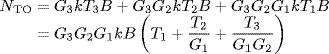
Now if Te is the effective input noise temperature of the cascaded arrangement of the three stages, which would have a gain of G3G2G1 as shown in Figure 7.9 (b), then the total noise power at the output (NTO) can also be computed from
Equating the two expressions for NTO gives
Generalizing the expression for n stages gives
The same expression can also be written in terms of noise figure specifications of individual stages as
where, F1, F2, F3 ... Fn are the noise figures for stages 1,2,3 ... n respectively and G1, G2, G3 ... Gn are the gains for stages 1,2,3 ... n respectively. It may be mentioned here that the gain values in the expression are not in decibels.
Figure 7.9 (a) Cascaded arrangement of three stages. (b) Equivalent single stage
The expressions for the noise figure and effective noise temperature derived above highlight the significance of the first stage. As is evident from these expressions, the noise performance of the overall system is largely governed by the noise performance of the first stage. That is why it is important to have the first stage with as low noise as possible.
7.6.5 Antenna Noise Temperature
The antenna noise temperature is a measure of the noise entering the receiver via the antenna. The antenna picks up noise radiated by various man-made and natural sources within its directional pattern. Various sources of noise, include noise generated by electrical equipment, noise emanating from natural sources including solar radiation, sky noise, background noise contributed by Earth, galactic noise due to electromagnetic waves emanating from radio stars in the galaxy and atmospheric noise caused by lightning flashes and absorption by oxygen and water vapour molecules followed by the re-emission of radiation.
Noise from these sources could enter the receiver both through the main lobe as well as through the side lobes of the directional pattern of the receiving antenna. Thus, the noise output from a receiving antenna is a function of the direction in which it is pointing, its directional pattern and the state of its environment. The noise performance of an antenna, as mentioned before, can be expressed in terms of a noise temperature called the antenna noise temperature. If the antenna noise temperature is TA K, it implies that the noise power output of the antenna is equal to the thermal noise power generated in a resistor at a temperature of TA K.
The noise temperature of the antenna can be computed by integrating the contributions of all the radiating bodies whose radiation lies within its directional pattern. It is given by
where
- θ = azimuth angle
- ϕ = elevation angle
- G(θ, ϕ) = antenna gain in the θ and ϕ directions
- Tb(θ, ϕ) = brightness temperature in the θ and ϕ directions
There are two possible situations to be considered here. One is that of the satellite antenna when the uplink is referred to and the other is that of the Earth station antenna when the downlink is referred to. These two cases need to be considered separately because of the different conditions that prevail both in terms of the antenna's directional pattern and the significant sources of noise.
In the case of satellite antenna (uplink scenario), the main sources of noise are Earth and outer space. Again, the noise contribution of the Earth depends upon the orbital position of the satellite and the antenna beam width. In case, the satellite antenna's beam width is more or less equal to the angle-of-view of Earth from the satellite, which is 17.5° for a geostationary satellite, the antenna noise temperature depends upon the frequency of operation and orbital position. In case the beam width is smaller as in case of a spot beam, the antenna noise temperature depends upon the frequency of operation and the area being covered on Earth. Different areas radiate different noise levels, as is obvious from Figure 7.10, which shows the brightness temperature model of the Earth in the Ku band.
Figure 7.10 Earth's brightness temperature model in the Ku band
In the case of the Earth station antenna (downlink scenario), the main sources of noise that contribute to the antenna noise temperature include the sky noise and the ground noise. The sky noise is primarily due to sources such as radiation from the sun and the moon and the absorption by oxygen and water vapour in the atmosphere accompanied by re-emission. The noise from other sources such as cosmic noise originating from hot gases of stars and interstellar matter, galactic noise due to electromagnetic waves emanating from radio stars in the galaxy is negligible at frequencies above 1 GHz. Here again there are two distinctly different conditions, one of clear sky devoid of any meteorological formations and the other that of sky with meteorological formations such as clouds, rain, etc.
In the clear sky conditions, the noise contribution is from sky noise and ground noise. The sky noise enters the system mainly through the main lobe of the antenna's directional pattern and the ground noise enters the system mainly through the side lobes and only partly through the main lobe, particularly at low elevation angles [Figure 7.11 (a)]. With reference to Figure 7.11 (b), if the attenuation and noise temperature figures for the meteorological formation are Am and Tm respectively, then the noise contribution due to sky noise is Tsky/Am and that due to the meteorological formation is Tm (1 − 1/Am).

Figure 7.11 Constituents of noise temperature of an Earth station antenna in (a) the clear sky condition and (b) the sky with meteorological formations
The sky noise contribution can be computed knowing the brightness temperature of the sky in the direction of the antenna within its beam width. Figure 7.12 illustrates a family of curves showing the brightness temperature of clear sky as a function of operating frequency for various practical elevation angles ranging from 5° to 60°. The contribution of ground noise can also be similarly computed knowing the brightness temperature of the ground. The brightness temperature of the ground may be as large as 290 K for a side lobe whose elevation angle is less than −10°, as shown in Figure 7.13 (a), and as small as 10 K for an elevation angle greater than 10°, as shown in Figure 7.13 (b).
Figure 7.12 Brightness temperature of the clear sky


Figure 7.13 Ground noise for elevation angles (a) less than −10° (b) Greater than 10°
In addition to the sky noise component discussed above, there are also a number of high intensity point sources in the sky noise. These sources subtend an angle that is only a few arcs of a minute and therefore they matter only if the Earth station antenna is highly directional and the radiation source lies within the antenna beam width.
The sky noise contribution increases significantly when heavenly bodies like the sun and the moon become aligned with the Earth station-satellite path. The increase in noise temperature is a function of operating frequency and the size of the antenna. The average noise temperature contribution due to the sun can be approximated as 12 000f−0.75, where f is the operating frequency in GHz. It may increase by a factor of 100 to 10 000 during the periods of high solar activity.
7.6.6 Overall System Noise Temperature
The overall system is a cascaded arrangement of the antenna, the feeder connecting the antenna output to the receiver input and the receiver as shown in Figure 7.14. Expressions can be written for the noise temperature at two points, one at the output of the antenna, i.e. input of the feeder, and second at the input of the receiver. The expression for the system noise temperature with reference to the output of the antenna (TSAO) can be written as
where
- TA = antenna noise temperature
- TF = thermodynamic temperature of the feeder, often taken as the ambient temperature
- LF = attenuation factor of the feeder
- Te = effective input noise temperature of the receiver
Figure 7.14 Computation of overall system noise temperature
The expression for the system noise temperature when referred to the receiver input (TSRI) can be written as
The above expression for the noise temperature takes into account the noise generated by the antenna and the feeder together with the receiver noise. The two expressions for the noise temperature given above highlight another very important point that the noise temperature at the antenna output is larger than the noise temperature at the receiver input by a factor of LF. This underlines the importance of having minimum losses before the first RF stage of the receiver.
7.7 Interference-related Problems
The major sources of interference were outlined in the introductory discussion on the topic in the earlier part of the chapter. These included:
- Intermodulation distortion
- Interference between the satellite and the terrestrial link sharing the same frequency band
- Interference between two satellites sharing the same frequency band
- Interference arising out of cross-polarization in frequency re-use systems
- Adjacent channel interference inherent to FDMA systems
Each of them will be briefly described in the following paragraphs.
7.7.1 Intermodulation Distortion
Intermodulation distortion is caused as a result of the generation of intermodulation products within the satellite transponder as a result of amplification of multiple carriers in the power amplifier, which is invariably a TWTA. The generation of intermodulation products is due to both amplitude nonlinearity and phase nonlinearity. Figure 7.15 shows the transfer characteristics (output power versus input power) of a typical TWTA. It is evident from the figure, that the characteristics are linear only up to a certain low input drive level and become increasingly nonlinear as the output power approaches saturation. Intermodulation products can be avoided by operating the amplifier in the linear region by reducing or backing off the input drive. A reduced input drive leads to a reduced output power. This results in a downlink power-limited system that is forced to operate at a reduced capacity.

Figure 7.15 Transfer characteristics of TWTA
Intermodulation products are generated whenever more than one signal is to be amplified by the amplifier with non-linear characteristics. Filtering helps to remove the intermodulation products but when these products are within the bandwidth of the amplifier, filtering is not of much use. The transfer characteristics of an amplifier can be written as
Where, A ![]() B
B ![]() C
C
It may be mentioned here that the intermodulation products are mainly generated by the third-order component in the equation as the third-order intermodulation products have frequencies close to the input frequencies and hence lie within the transponder bandwidth.
Let us consider that the signal applied to the input of the amplifier is given by
In other words, two unmodulated carriers at frequencies f1 and f2 are applied to the input of the amplifier.
The output of the amplifier is given by
The first term is the linear term and it amplifies the input signal by A and represents the desired output of the amplifier (V desout).
The total desired power output from the amplifier, referenced to a one ohm load is, therefore given by
Where,
- P1 = 1/2(
 )
) - P2 = 1/2(
 )
)
The second term in equation 7.38 is the second order term and can be expanded as
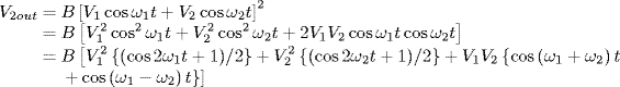
The term V2out contains frequency components 2f1, 2f2, (f1 + f2) and (f1 − f2). All these components can be removed from the amplifier output with the help of band pass filters.
The third term in the equation 7.38 is the third order term and can be expanded as

The first two terms contain frequency components f1, f2, 3f1 and 3f2. The triple frequency component can be removed from the amplifier output with the help of band pass filters. The fifth and the last terms contain the frequency components (2f1 + f2) and (2f2 + f1) which can again be removed by the band pass filters. The frequency components (2f1 − f2) and (2f2 − f1) in the fourth and seventh terms can fall within the bandwidth of the transponder and are referred to as third-order intermodulation products of the amplifier. Therefore, the intermodulation products of concern are
The power of the intermodulation components is given by
It is clear from the equation 7.42 that the ratio of intermodulation power to the desired power increase in proportion to the cubes of the signal power and also to square of (C/A). The greater the non-linearity of the amplifier, larger is the value of (C/A) and larger the value of intermodulation products. Also, the intermodulation terms increase rapidly as the amplifier operates near its saturation region.
The easiest way to reduce the intermodulation problems is to reduce the levels of input signals to the amplifier. The output backoff is defined as the difference in decibels between the saturated output power of the amplifier and its actual power. When the transponder is operated with output backoff, the power level at the input is reduced by input backoff. As the characteristics of the amplifier are non-linear, the value of input backoff is greater than the value of output backoff.
The overall C/N ratio taking into account the contribution of intermodulation products is given by
Intermodulation distortion is a serious problem when the transponder is made to handle two or more carrier signals. That is why satellite links that use frequency division multiple access technique are particularly prone to this type of interference. On the other hand, a single carrier per transponder TDMA system is becoming increasingly popular as in this case the satellite TWTA can be operated at or close to the saturation level without any risk of generating intermodulation products. This maximizes the EIRP for the downlink.
Another intermodulation interference-related problem associated with the FDMA system is that the Earth station needs to exercise a greater control over the transmitted power in order to minimize the overdrive of the satellite transponder and the consequent increase in intermodulation interference. Intermodulation considerations also apply to Earth stations transmitting multiple carriers, which forces the amplifiers at the Earth station to remain underutilized.
7.7.2 Interference between the Satellite and Terrestrial Links
Satellite and terrestrial microwave communication links cause interference to each other when they share a common frequency band. The 6/4 GHz frequency band is allocated to both the satellite as well as terrestrial microwave links. An Earth station receiving at 4 GHz is susceptible to interference from terrestrial stations transmitting at 4 GHz. Similarly, an Earth station transmitting at 6 GHz is a source of interference for a terrestrial station receiving at 6 GHz. The level of mutual interference between the two is a function of a number of parameters including carrier power, carrier power spectral density and the frequency offset between the two carriers.
The level of interference caused by a terrestrial transmission to a satellite signal reception would depend upon the spectral density of the terrestrial interfering signal and the bandwidth of the satellite signal received by the Earth station. As an example, for a broadband satellite signal, the whole of the interfering carrier power may be applicable whereas for a narrowband satellite signal, the interfering carrier power is reduced by a factor equal to the ratio of the total carrier power and the carrier power included in the narrow bandwidth.
Interference from a narrowband satellite transmission to a terrestrial microwave system can be reduced by using a frequency offset between the satellite and terrestrial carriers. The amount of interference depends upon the frequency difference between the interfering satellite carrier frequency and the terrestrial carrier frequency. The interference reduction factor in this case can be determined by convolving the power spectral densities of the interfering satellite carrier signal and the terrestrial carrier signal.
7.7.3 Interference due to Adjacent Satellites
This type of interference is caused by the presence of side lobes in addition to the desired main lobe in the radiation pattern of the Earth station antenna. If the angular separation between two adjacent satellite systems is not too large, it is quite possible that the power radiated through the side lobes of the antenna's radiation pattern, whose main lobe is directed towards the intended satellite, interferes with the received signal of the adjacent satellite system. Similarly, transmission from an adjacent satellite can interfere with the reception of an Earth station through the side lobes of its receiving antenna's radiation pattern.
This type of interference phenomenon is illustrated in Figure 7.16. Satellite A and satellite B are two adjacent satellites. The transmitting Earth station of satellite A on its uplink, in addition to directing its radiated power towards the intended satellite through the main lobe of its transmitting antenna's radiation pattern, also sends some power, though unintentionally, towards satellite B through the side lobe. The desired and undesired paths are shown by solid and dotted lines respectively. In the figure, θ is the angular separation between two satellites as viewed by the Earth stations and β is the angular separation between the satellites as viewed from the centre of the Earth; i.e. β is simply the difference in longitudinal positions of the two satellites. Coming back to the problem of interference, transmission from satellite B on its downlink, in addition to being received by its intended Earth station shown by a solid line again, also finds its way to the receiving antenna of the undesired Earth station through the side lobe shown by the dotted line. Quite obviously, this would happen if the off-axis angle of the radiation pattern of the Earth station antenna is equal to or more than the angular separation θ between the adjacent satellites. θ and β are interrelated by the following expression:
where
- dA = slant range of satellite A
- dB = slant range of satellite B
- r = geostationary orbit radius

Figure 7.16 Interference due to adjacent satellites
For a known value of θ, the worst case acceptable value of the off-axis angle of the antenna's radiation pattern can be computed. Similarly, for a given radiation pattern and known off-axis angle, it is possible to find the minimum required angular separation between the two adjacent satellites for them to coexist without causing interference to each other. Let us take the case of downlink interference and determine the expression for carrier-to-interference (C/I) ratio.
The desired carrier power CD for the downlink channel in dBW can be expressed as
where
- EIRP = desired EIRP(in dBW, or decibels relative to a power level of 1 W)
- LD = downlink path loss for the beam from the desired satellite(in dB)
- G = Earth station antenna gain in the direction of the desired satellite(in dB)
The interfering carrier power for the downlink channel (ID) in dBW is given by
where
- EIRP′ = interfering EIRP(in dBW)
 = downlink path loss for the beam from interfering satellite(in dB)
- G′ = Earth station antenna gain in the direction of the interfering satellite(in dB)
The expression for (C/I) in the case of downlink can then be written as
where (C/I)D is the C/I for the downlink channel in dB.
If the path losses are considered as identical, then
Also, the term (G − G′) is the receive Earth station antenna discrimination, which is defined as the antenna gain in the direction of the desired satellite minus the antenna gain in the direction of the interfering satellite. According to CCIR standards, in cases where the ratio of the antenna diameter to the operating wavelength is greater than 100, G′ as a function of the off-axis angle θ should at the most be equal to (32 − 25 log θ) dB (forward gain of an antenna compared to an idealized isotropic antenna), where θ is in degrees. The requirement of FCC standards for the same is (29 − 25 log θ) dB. Figure 7.17 shows the typical Earth station antenna pattern, which is a plot of the gain versus the off-axis angle along with CCIR requirements. This gives
A similar calculation can be made for the uplink interference, where a satellite may receive an unwanted signal from an interfering Earth station. In the case of uplink, the expression for C/I can be written as

Figure 7.17 Typical Earth station antenna pattern
where
- (C/I)U = C/I for the uplink channel in dB
- EIRP = EIRP of the desired Earth station in dBW
- EIRP′ = EIRP of the interfering Earth station in the direction of the satellite in dBW
- G = gain of the satellite receiving antenna in the direction of the desired Earth station in dB
- G′ = gain of the satellite receiving antenna in the direction of the interfering Earth station in dB
EIRP′ is further equal to
where
- EIRP∗ = EIRP of the interfering Earth station in dBW
- GI = on-axis transmit antenna gain of the interfering Earth station in dB
- θ = viewing angle of the satellite from the desired and interfering Earth Stations
The overall carrier-to-interference ratio (C/I) for adjacent satellite interference is given by
where the subscripts U and D imply uplink and downlink respectively. Where the interference is noise like, it is possible to combine the effects of noise and interference. The combined carrier-to-noise ratio ![]() is given by
is given by
It may be mentioned here that the various terms in equations 7.52 and 7.53 are not in decibels.
7.7.4 Cross-polarization Interference
Cross-polarization interference occurs in frequency re-use satellite systems. It occurs due to coupling of energy from one polarization state to the other orthogonally polarized state in communications systems that employ orthogonal linear polarizations (horizontal and vertical polarization) and orthogonal circular polarizations (right-hand circular and left-hand circular). The coupling of energy from one polarization state to the other polarization state takes place due to finite cross-polarization discrimination of the Earth station and satellite antennas and also by depolarization caused by rain, particularly at frequencies above 10 GHz.
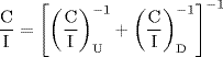
Cross-polarization discrimination is defined as the ratio of power received by the antenna in principal polarization to that received in orthogonal polarization from the same incident signal. A cross-polarization discrimination figure of 30 to 40 dB along the antenna axis is considered very good. The combined effect of finite values of cross-polarization discrimination for the Earth station and satellite antennas can be expressed in the form of net minimum cross-polarization discrimination for the overall link as follows:
where X is the worst case carrier-to-cross polarization interference ratio. Xe and Xs are the cross-polarization discrimination for the Earth station antenna and for the satellite antenna respectively. It can be taken as an additional source of interference while computing the overall carrier-to-noise plus interference ratio.
7.7.5 Adjacent Channel Interference
Adjacent channel interference occurs when the transponder bandwidth is simultaneously shared by multiple carriers having closely spaced centre frequencies within the transponder bandwidth. When the satellite transmits to Earth stations lying within its footprint, different carriers are filtered by the receiver so that each Earth station receives its intended signal. Filtering would have been easier to realize had there been a large guard band between adjacent channels, which is not practically feasible as that would lead to the inefficient use of the transponder bandwidth. The net result is that a part of the power of the carrier in the channel adjacent to the desired one is also captured by the receiver due to overlapping amplitude characteristics of the channel filters. This becomes a source of noise.
7.8 Antenna Gain-to-Noise Temperature (G/T) Ratio
The antenna gain-to-noise temperature (G/T) ratio, usually defined with respect to the Earth station receiving antenna, is an indicator of the sensitivity of the antenna to the downlink carrier signal from the satellite. It is a figure-of-merit used to indicate the combined performance of the Earth station antenna and low noise amplifier combined in receiving weak carrier signals. G is the receive antenna gain, usually referred to the input of the low noise amplifier. It equals the receive antenna gain as computed, for instance, from G = η(4πAe/λ2) minus the power loss in the waveguide connecting the output of the antenna to the input of the low noise amplifier. T is the Earth station effective noise temperature, also referred to as the noise temperature at the input of the low noise amplifier. It may be mentioned here that the value of the G/T ratio is invariant irrespective of the reference point chosen to measure its value. The input of the low noise amplifier is chosen because it is the point where its contribution is clearly shown.
During the discussion on system noise temperature earlier in the chapter, expressions were derived for the overall system noise temperature as referred to the output of the receive antenna as well as the input of the low noise amplifier. The system noise temperature at the output of the antenna (TSAO) was derived as
where
- TA = antenna noise temperature
- TF = thermodynamic temperature of the feeder, often taken as the ambient temperature
- LF = attenuation factor of the feeder
- Te = effective input noise temperature of the receiver
The system noise temperature when referred to the input of the low noise amplifier (TSRI) was derived as
where Te can further be expressed as
Here, T1, T2 and T3 are the noise temperatures of different stages in the receiver, beginning with the low noise amplifier, and G1, G2 and G3 are the corresponding gain values.
From the known values for G and T, the G/T ratio can be computed. To conclude the discussion on the G/T ratio, the following observations can be made:
- The higher the antenna gain and the lower the loss of the feeder connecting the output of the antenna to the input of the low noise amplifier, the higher will be the G/T ratio.
- The lower the noise temperature of the low noise amplifier, the higher will be the G/T ratio.
- The higher the gain of the low noise amplifier, the lower will be the noise contribution of successive stages in the receiver and the higher will be the G/T ratio.
7.9 Link Design
The design of any satellite based communication system is based on the two objectives of meeting a minimum C/N ratio for a specified time period and carrying maximum traffic at minimum cost. Both of these objectives are contradictory and the art of system design is to reach the best compromise so as to meet all the system parameters at minimum cost.
There are many parameters that affect the design of a satellite based communication system. These parameters may be categorized according the sub-system to which they are of prime importance (Earth station, satellite and satellite-Earth station channel). The parameters related to the Earth station design are geographical location of the Earth station (which provides an estimate of rain fades, satellite look angle, satellite EIRP and path loss), transmit antenna gain and transmitter power, receive antenna gain, system noise temperature and characteristics of the different modules of the Earth station (demodulator characteristics, filter characteristics, cross-polarization discrimination). Satellite related parameters are location of the satellite (determines the coverage region and Earth station look angle), transmit antenna gain, radiation pattern and transmitted power, receive antenna gain and radiation pattern and transponder, type, gain and its noise characteristics. The parameters of the transmission channel that affect the link design are operating frequency (path loss and link margin) and propagation characteristics (decide the link margin and choice of modulation and coding). A one way satellite link consists of two separate paths; an up-link path from the Earth station to the satellite and a down-link path from the satellite to the Earth station. A typical two way satellite link comprises of four separate paths; an uplink path from the first Earth station to the satellite, downlink path from the satellite to the second Earth station, uplink from the second Earth station to the satellite and a downlink from the satellite to the first Earth station. The design procedure for a one way satellite link is highlighted in the following paragraphs. The design for a two way link can also be carried out on similar lines.
7.9.1 Link Design Procedure
The satellite communication link design procedure is as follows:
- Determine the frequency band in which the system will operate.
- Determine the communication parameters of the satellite.
- Calculate the signal-to-noise ratio and the bit error rate for the baseband channel.
- Determine the parameters of the transmitting and the receiving Earth stations.
- The design starts with the transmitting Earth station. Determine the carrier-to-noise ratio for the uplink using the uplink budget and the transponder noise power budget.
- Determine the output power of the transponder based on the value of the transponder gain.
- Determine the carrier-to-noise ratio for the downlink and establish the noise budget for the receiving Earth station at the edge of the coverage zone.
- Determine the propagation conditions under which the system operates and calculate the value of atmospheric attenuation and other losses caused due to the atmospheric conditions.
- Determine the link margin by calculating the link budget. Compare the result with the desired specifications. Change the system parameters to obtain the desired value of the link margin.
7.9.2 Link Budget
The link budget is a way of analysing and predicting the performance of a microwave communication link for given values of vital link parameters that contribute to either signal gain or signal loss. It is the algebraic sum of all gains and losses expressed in decibels as we move from the transmitter to the receiver. The final value thus obtained provides us with the means of knowing the available signal strength at the receiver and therefore also knowing how strong the received signal is with respect to the minimum acceptable level, called the threshold level. The difference between the actual value and the threshold is known as the link margin. The higher the value of the link margin, the better is the quality of the microwave link. The link budget is thus a tool that can be used for optimizing various link parameters in order to get the desired performance.
The concept of the link budget can be illustrated further with the help of a one-way microwave communication link schematic shown in Figure 7.22. Various parameters of interest in this case would be:
Figure 7.22 Link budget
- Transmitter power PT
- Power loss in the waveguide connecting the transmitter output to the antenna input LT
- Transmitting antenna gain GT
- Free-space path loss LP
- Attenuation due to rain, clouds, fog, etc., A
- Receive antenna gain GR
- Power loss in the waveguide connecting the receive antenna output to the receiver input LR
- Received signal power PR
The power balance equation describing the link budget in this case would be given by
It may be mentioned here that all the power levels in the above expression are in dBW and the gain, attenuation and loss terms are in dB.With reference to a satellite link, such an equation can be written for both the uplink as well as the downlink. Figure 7.23 shows the schematic arrangement of a satellite link indicating various parameters that typically contribute to the link budget. For the satellite link shown in Figure 7.23, the uplink and downlink power balance equations can be written as
Design of the uplink channel is often easier than the downlink channel as higher power transmitters can be placed on the Earth stations than on the satellites. However, there are some systems like the VSATs which have limitations on the size of the antennas that can be used on the Earth station. The design of the uplink channel is done with the aim of producing a certain flux density or a certain power level at the input of the satellite transponder. The desired EIRP of the transmitting Earth station is calculated based on this requirement.
The design of the downlink channel is done by taking into consideration the back-off requirements of the satellite transponder amplifier to reduce the intermodulation problems. This is made possible either by reducing the uplink transmitter power or by reducing the satellite transponder amplification.
As an example, let us look at the link budget of a typical Ku band satellite-to-DTH receiver downlink. Typical values for the various parameters are:
- Transmit power PTD = 25 dBW
- Transmit waveguide loss LTD = 1 dB
- Transmit antenna gain GTD = 30 dB
- Free-space path loss LPD = 205 dB
- Receive antenna gain GRD (for a 50 cm diameter dish) = 39.35 dB
- Receive waveguide loss LRD = 0.5 dB
The received signal power can be computed from the above data to be equal to −112.15 dBW. If the receive system noise temperature is taken to be 140 K and the receive bandwidth to be 27 MHz, which are typical values for the link under consideration, then the receiver noise power would be
Therefore, the received carrier-to-noise C/N ratio for this link would be 20.68 dB. This figure can be used to determine the link margin and hence the quality of service provided by the link under clear sky conditions. It can also be used to assess the deterioration in the quality of service in case of hostile atmospheric conditions.
7.10 Multiple Spot Beam Technology
Multiple spot beam technology is a concept in broadband satellite communications that allows frequency reuse, thereby maximizing the bandwidth capacity and minimizing the required frequency allocation. Inherent to the operational concept of multiple spot beam technology and the related frequency reuse feature is the capability of the satellite employing the technology to transmit multiple streams of information using the same frequency without causing unwanted interference. With increase in demand for satellite capacity, the traditional broadcast satellite technology operating on Ku-band becomes a limiting factor. Due to a large footprint at Ku-band, which would be much larger than what it would be at Ka-band for the same antenna size, the traditional Ku-band satellites do not support flexible distribution of the bandwidth required in the case of broadband internet.
While Ku-band is from 12 to 18 GHz, Ka-band extends from 26.5 to 40 GHz, including the upper part of the super high frequency (SHF) band of 3–30 GHz and the lower part of the extremely high frequency (EHF) band of 30–300 GHz. Typically, 27.5–30 GHz is used for uplink transmissions and 17.7–20.2 GHz is used for downlink transmissions. For a given antenna size, Ka-band operation provides higher gain and narrower beam width, leading to a much smaller footprint on Earth. This allows deployment of multiple beams to cover a given area. Figure 7.24 shows a comparison between use of a single large beam and multiple spot beams to provide the same coverage.
Figure 7.24 Comparison between (a) single large beam and (b) multiple spot beams to cover a given area
While a traditional Ku-band satellite may use a single downlink beam to cover a given area on Earth, a Ka-band satellite uses multiple spot beams to provide the same coverage. The multiple spot beam concept of covering a larger area is analogous to a cellular telephone network with each of the spot beams corresponding to a cell. It may be mentioned here that if one uses a single wide beam to cover the whole of a very large geographical area, then one can transmit the same information to every receiver in that area tuned to receive that information at the same time. The limitation is that only one stream of information can be transmitted at a time, which is fine with applications such as live television broadcasts. This would not be an efficient mode of communication for internet transmissions.
Use of multiple spot beams with each beam covering a small well-defined area in the larger area to be covered implies that multiple streams of information can be transmitted using the same frequency. This allows services to be provided to many more customers with one satellite.
There are a large number of communication satellites that employ multiple spot beam technology. It may also be mentioned here that not all spot beam services are equivalent and that different satellite operators are using spot beam technology at both Ku-band and Ka-band for various purposes. Ka-band operation of course allows a much smaller footprint with the result that multiple spot beam Ka-band satellites have increased capacity as compared to Ku-band satellites. Ka-band satellites employing multiple spot beam technology are also sometimes called high throughput satellites (HTS). HTSs are defined as a class of communication satellites that provide at least twice the total throughput of a classical fixed satellite service (FSS) satellite for the same allocated spectrum. The throughput of an HTS is usually greater by a factor of 20 or more.
Some of the well-known communication Ka-band satellites employing multiple spot beam technology include Spaceway-3 and EchoStar-17, also known as Jupiter-1 and Spaceway-4, from the EchoStar Corporation, Anik-F2 from Telesat Canada, KA-SAT from Eutelsat, Yahsat Y1B from AlYahsat, Thaicom-4 from Thaicom Public Company Ltd, ViaSat-1 from ViaSat, Astra-2E from Astra Communications and HYLAS-2 from Avanti Communications.
Spaceway-3 from Hughes Network Systems, a subsidiary of EchoStar Corporation, is one of the largest operational Ka-band satellite networks in the world and is also the first with onboard switching and routing. With 10 Gbps capacity, it enables communications directly between customer locations in a single hop without requiring a central hub. EchoStar-17 is also a geostationary communications satellite operated by Hughes Network Systems and used for satellite broadband. It has 60 Ka-band transponders that produce 60 narrow downlink beams to deliver broadband satellite services in North America.
Anik-F2 from Telesat, Canada is a communications satellite providing Ka-band multimedia services across North America in addition to offering an FSS service including internet access. It has a total of 114 transponders, including 50 operating in Ka-band, 40 in Ku-band and 24 in C-band.
Eutelsat's KA-SAT is Europe's HTS providing 82 Ka-band spot beams connected to a network of 10 ground stations. The configuration allows frequency reuse, thereby increasing the throughput beyond 90 Gbps. Figure 7.25 shows use of multiple spot beams by KA-SAT to cover Europe.

Figure 7.25 KA-SAT employing multiple spot beam technology covering Europe
Yahsat-Y1B from AlYahsat is a communications satellite equipped with 25 110 MHz transponders to provide a high speed internet service to south-west Asia, the Middle East, Africa and Eastern Europe using multiple spot beam technology.
Thaicom-4, also called IPSTAR, is a broadband communications satellite designed for high speed internet/multimedia services. The satellite has a capacity of 45 Gbps. Its multiple spot beam technology offers 20 times higher bandwidth compared to traditional Ku-band satellites.
ViaSat-1 from ViaSat is a high capacity communications satellite with a capacity exceeding 140 Gbps. It is equipped with 56 Ka-band transponders that provide broadband internet services to North America. ViaSat-2 is scheduled to be launched during 2016 and will further augment capacity and coverage area.
Astra-2E from Astra Communications is a communications satellite designed to provide free-to-air and encrypted direct-to-home (DTH) digital television and satellite broadband services for Europe and the Middle East. The satellite has three Ku-band downlink beams with two of them covering Europe and the third covering the Middle East. The Ka-band footprint spreads across Europe.
HYLAS-2 (Highly Adaptable Satellite) from Avanti Communications is a high throughput communications satellite equipped with 24 active Ka-band transponders producing 24 Ka-band downlink beams, which along with four gateway beams provide two-way communications services such as corporate networking, broadband internet access, business continuity services and video distribution. The satellite provides coverage to northern and southern Africa, Eastern Europe and the Middle East, and is also equipped with steerable spot beam to provide coverage anywhere on Earth within the spacecraft's visibility.
Further Readings
- Calcutt, D. and Tetley, L. (1994) Satellite Communications: Principles and Application, Edward Arnold, a member of the Hodder Headline Group, London.
- Chartant, R.M. (2004) Satellite Communications for the Nonspecialist, SPIE, Washington.
- Elbert, B.R. (1997) The Satellite Communication Applications Handbook, Artech House, Boston, Massachusetts.
- Elbert, B.R. (1999) Introduction to Satellite Communication, Altech House, Boston, Massachusetts.
- Elbert, R.B. (2001) Satellite Communication Ground Segment and Earth Station Handbook, Artech House, Boston, Massachusetts.
- Gedney, R.T., Schertler, R. and Gargione, F. (2000) Advanced Communications Technology Satellite: Insider's Account of the Emergence of Interactive Broadband Services in Space, SciTech, New Jersey.
- Gedney, R.T., Schertler, R. and Gargione, F. (2000) Advanced Communication Technology, SciTech, New Jersey.
- Geoffrey, L.E. Communication Services via Satellite, Butterworth Heinemann, Oxford.
- Inglis, A.F. (1997) Satellite Technology: An Introduction, Butterworth Heinemann, Massachusetts.
- Kadish, J.E. (2000) Satellite Communications Fundamentals, Artech House, Boston, Massachusetts.
- Maral, G. and Bousquet, M. (2002) Satellite Communication Systems: Systems, Techniques and Technology, John Wiley & Sons, Ltd, Chichester.
- Pattan, B. (1993) Satellite Systems: Principles and Technologies, Van Nostrand Reinhold, New York.
- Perez, R. (1998) Wireless Communications Design Handbook: Space Interference, Academic Press, London.
- Richharia, M. (1999) Satellite Communication Systems, Macmillan Press Ltd. Richharia, M. (2001) Mobile Satellite Communications: Principles and Trends, Addison Wesley.
- Sherrif, R.E. and Hu, Y.F. Mobile Satellite Communication Networks, John Wiley & Sons, Ltd, Chichester.
Internet Sites
- http://www.satsig.net/linkbugt.htm
- http://engr.nmsu.edu/~etti/spring97/communications/nsn/linkbudget.html
- http://en.wikipedia.org/wiki/Thermal_noise
- http://www.satsig.net/noise.htm
- http://homes.esat.kuleuven.be/~cuypers/satellite_noise.pdf
- http://www.tutorialsweb.com/satcom/link-power-budget/uplink-noise-ratio.htm
Glossary
- Anik-F2:
- high throughput communications satellite from Telesat Canada
- Antenna gain-to-noise temperature (G/T) ratio:
- This is usually defined with respect to the Earth station receiving antenna and is an indicator of the sensitivity of the antenna to the downlink carrier signal from the satellite. It is the figure-of-merit used to indicate the performance of the Earth station antenna and low noise amplifier combined to receive weak carrier signals
- Antenna noise temperature:
- This is a measure of noise entering the receiver via the antenna. The noise temperature of the antenna can be computed by integrating contributions of all the radiating bodies whose radiation lies within the directional pattern of the antenna
- Astra-2E:
- Communications satellite from Astra Communications
- Broadcast Satellite Services (BSS):
- This refers to the satellite services that can be received at many unspecified locations by relatively simple receive-only Earth stations
- Cross-polarization discrimination:
- This is defined as the ratio of power received by the antenna in principal polarization to that received in orthogonal polarization from the same incident signal
- Cross-polarization interference:
- This occurs in frequency re-use satellite systems. It occurs due to coupling of energy from one polarization state to the other orthogonally polarized state in communications systems that employ orthogonal linear polarizations (horizontal and vertical polarization) and orthogonal circular polarizations (right-hand circular and left hand circular). The coupling of energy from one polarization state to the other polarization state takes place due to finite values of cross-polarization discrimination of the Earth station and satellite antennas and also by depolarization caused by rain, particularly at frequencies above 10 GHz
- Fixed Satellite Services (FSS):
- This refers to the two-way communication between two Earth stations at fixed locations via a satellite
- Free-space loss:
- This is the loss of signal strength due to the distance from the transmitter. While free space is a theoretical concept of space devoid of all matter, in the present context it implies remoteness from all material objects or forms of matter that could influence propagation of electromagnetic waves
- High throughput satellite (HTS):
- A class of communication satellites that provide at least twice the total throughput of a classical fixed satellite service satellite from the same allocated spectrum
- HYLAS-2:
- High throughput communications satellite from Avanti Communications
- Intermodulation interference:
- This is caused due to generation of intermodulation products within the satellite transponder as a result of amplification of multiple carriers in the power amplifier, which is invariably a TWTA
- Johnson noise:
- Another name for thermal noise or white noise
- KA-SAT:
- Eutelsat's high throughput satellite
- Link budget:
- This is a way of analysing and predicting the performance of a microwave communication link for given values of vital link parameters that contribute to either signal gain or signal loss. It is the algebraic sum of all gains and losses expressed in decibels when travelling from the transmitter to the receiver
- Mobile Satellite Services (MSS):
- This refers to the reception by receivers that are in motion, like ships, cars, lorries, and so on.
- Multiple spot beam technology:
- A concept in broadband satellite communications that allows frequency reuse to maximize bandwidth capacity and minimize required frequency allocation
- Noise figure:
- It is defined as the proportion of the signal-to-noise ratio at the input of the amplifier to the signal-to-noise ratio at its output
- Noise temperature:
- This is just another way of expressing the noise performance of a device in terms of its equivalent noise temperature. It is the temperature of a resistance that would generate the same noise power at the output of an ideal (i.e. noiseless) device as that produced at its output by an actual device when terminated at its input by a noiseless resistance, that is a resistance at absolute zero temperature
- Polarization rotation:
- When an electromagnetic wave passes through a region of high electron content, such as ionosphere, the plane of polarization of the wave is rotated due to interaction of the electromagnetic wave and the Earth's magnetic field. The angle through which the plane of polarization rotates is directly proportional to the total electron content of the ionosphere and inversely proportional to the square of the operating frequency. It also depends upon the state of the ionosphere, time of the day, solar activity, direction of the incident wave, etc. The directions of polarization rotation are opposite for transmit and receive signals
- Scintillation:
- This is simply the rapid fluctuation of the signal amplitude, phase, polarization or angle of arrival. In the ionosphere, scintillation occurs due to small scale refractive index variations caused by local ion concentration. The scintillation effect is inversely proportional to the square of the operating frequency and is predominant at lower microwave frequencies, typically below 4 GHz
- Spaceway-3:
- A high throughput satellite from EchoStar Corporation
- Thaicom-4:
- Broadband communications satellite designed for high speed internet/multimedia services
- Thermal noise:
- Thermal noise is generated in any resistor or resistive component of any impedance due to the random motion of molecules, atoms and electrons. It is called thermal noise as the temperature of a body is the statistical RMS value of the velocity of motion of these particles. It is also called white noise as, due to the randomness of the motion of particles, the noise power is evenly spread over the entire frequency spectrum
- ViaSat-1:
- High capacity communications satellite from ViaSat
- White noise:
- Another name for thermal noise or Johnson noise
- Yahsat-Y1B:
- Communications satellite from AlYahsat