
12 Principles for secure encryption
- Five principles for secure encryption
- Large blocks and long keys
- Confusion, or non-linearity
- Diffusion and saturation
Let’s pull together everything we learned in chapter 11. In sections 12.1 to 12.5 we will distill the 5 underlying principles that make a block cipher secure. One hallmark of a secure block cipher is that changing any bit in the key or any bit in the plaintext will cause about 50% of the bits in the ciphertext block to change, preferably in a random-looking pattern. Changing any other bit also will cause about 50% of the bits in the ciphertext block to change, but in a different pattern. Let’s call this the Fifty-Fifty property. This chapter will describe how to make that happen.
12.1 Large blocks
We have seen that a bigram cipher can be solved just like a simple substitution cipher by compiling bigram frequencies and contact frequencies. This can also be done for trigrams and tetragrams, although a very large amount of ciphertext is needed. For block ciphers done by hand, the smallest block size that should be considered is 5 characters. For computer ciphers the minimum block size is 8 bytes. One purpose of a large block size is to prevent Emily from solving the cipher like a code. That is, Emily would find repeated ciphertext blocks and deduce their meaning from their frequency and their positions in the message. To take an extreme case, if the block size is 1 character, then no matter how large the key is, and how many encryption steps are used, the cipher is still just a simple substitution.
There are numerous 8-character sequences in English that are common enough to appear repeatedly in a long message. Here are a dozen examples, using an ellipsis ... to represent a blank space.

Today’s standard block size is 16 bytes. There is no high-frequency English phrase that long. There could be some long contextual phrases such as UNITED STATES GOVERNMENT, EXECUTIVE COMMITTEE, INTERNATIONAL WATERS, and so forth. However, to produce repeated ciphertext blocks, these plaintext repeats must align the same way with the block boundaries. For example, 16-byte plaintext blocks UNITED...STATES...GO and NITED...STATES...GOV would not produce recognizable ciphertext repeats when you are using a strong block cipher.
The problem of repeated ciphertext blocks disappears when you use block chaining (section 11.9). With block chaining, any block size 8 bytes or longer, can be used.
12.2 Long keys
We know that a secure cipher must have a large key to prevent a brute-force attack. The current standard is a 128-bit key. If you need your messages to remain secret for 20 years or longer, I recommend a minimum of 160 bits. That is equivalent to about 48 decimal digits, 40 hexadecimal digits or 34 single-case letters.
If you are typing the key by hand, I suggest that you structure your keys in a uniform way. Divide the key into blocks of equal size with a consistent format. Here are two styles of uniformly structured keys. In the first style, all of the characters in each block are the same type, uppercase letters, lowercase letters or digits. In the second style, the blocks have the same format, 2 uppercase letters and 3 digits.
![]()
The first of these two keys is equivalent to about 191 bits, and the second is equivalent to about 174 bits. For long keys like these you must be able to see the characters while you are typing, so that you can review them and make corrections when needed. When the key is complete, the application should display a checksum so you can verify that the key is correct.
One advantage of this regularity is that it prevents mistaking a letter O for a digit 0, or a letter I for a digit 1. I do not recommend random mixing of characters, like $v94H;t}=Nd^8, because it leads to mistakes. If you have a data file encrypted using the key $v94H;t}=Nd^8 and you decrypted it using the key $V94H;t}=Nd^8, that data file could now be unrecoverable. You may never figure out what went wrong and how to fix it. Using uniform blocks in your keys helps prevent such disasters.
Another form of key that helps to prevent typing errors is artificial words. Make up your own pronounceable letter combinations, like this:
![]()
Try to avoid patterns, such as using the same vowel combinations, palek mafner vadel glabet, and the like, where all of the words use the A-E vowel pattern.
These alphanumeric keys can be converted into binary form by software. The madd ripple cipher (section 11.8) is well-suited for this task.
An alternative to typing the keyword for each message or data file that gets encrypted is to use a keyword manager that generates the keywords and associates them with the messages or files. The keyword manager could be installed on a website accessible to both Sandra and Riva. This topic will not be covered in this book. Note that a keyword manager is different from a password manager because Sandra and Riva, working on different computers, must use the same keyword for each file.
12.2.1 Redundant keys
In some cases it may be possible for Emily to devise equations that relate the ciphertext to the plaintext and the key. If Emily knows, or can guess, some of the plaintext, these equations may make it possible for her to determine the key. For example, she may know that some of the messages begin with ATTENTION in all-cap letters. This might be sufficient for her to solve a 64-bit key when an 8-byte block size is used.
One way to defeat this potential attack is to enlarge the key. For example, if the block size is 64 bits, but the key is 32 bits larger, namely 96 bits, then you would expect, on average, that there would be about 232 possible keys that transform the known plaintext into the ciphertext. Emily would need to sift through these 232 solutions to find the correct one. This could be a difficult task because many of the more than 4,000,000,000 possibilities could look like plausible text.
Enlarging the key will make Emily’s task much harder, but not necessarily impossible. If she has twice as much known plaintext, then the equations for two cipher blocks might be used to solve for the key. However, it is much rarer to have that much known plaintext, and solving twice as many equations may take far longer than merely twice as long. Depending on the type of equations Emily is using, it may be feasible to solve a set of 64 equations, but not a set of 128 equations.
If Emily does not have solvable equations, then redundant keys serve to make a brute-force attack far more difficult and costly. Either way, redundant keys make Emily work harder.
12.3 Confusion
In 1945 Claude Shannon, the founder of information theory, described two properties that a strong cipher must possess. He called these confusion and diffusion. By confusion, Shannon meant that there should not be a strong correlation between the plaintext and the ciphertext. Likewise, there should not be a strong correlation between the key and the ciphertext. By diffusion, Shannon meant that every part of the ciphertext should depend on every part of the plaintext and every part of the key.
There is a third property that I will add to Shannon’s two. I call this property saturation. The idea is to measure how strongly each bit or byte of the ciphertext depends on each bit or byte of the plaintext and the key. The greater the saturation, the stronger the cipher. This section, and the following two sections, will discuss these three properties, confusion, diffusion and saturation, in detail.
There are two types of substitutions that are used in block ciphers, fixed and keyed. Keyed substitutions are variable, and can be changed for each message, or even each block. There is a discussion of the pros and cons of these methods in section 11.6. If you decide to use a keyed substitution, or if you find the math in this section difficult, then you can skip ahead to section 12.4. You can construct your mixed alphabet or tableau using the SkipMix algorithm described in sections 5.2 and 12.3.7 and choose the sequence of skips using a pseudorandom number generator.
Confusion, in Shannon’s sense, is basically an issue of linearity versus non-linearity. If your block cipher uses a fixed alphabet or tableau, linearity is of paramount importance. The entire field of linear algebra is based on the concept of linearity. The term linearity comes from analytic geometry. The equation for a straight line is ax+by = c, where a, b and c are constants and the variables x and y represent the Cartesian coordinates of a point on a line. If the line is not parallel to the y-axis, the equation can be expressed as y = ax+b. Both ax+by = c and y = ax+b are examples of linear equations, or linear relationships.
The Caesar cipher (section 4.2) is an example of a linear cipher. The Caesar cipher may be regarded as adding the key to the plaintext to get the ciphertext, c = p+k. Here c is the ciphertext letter, p is the plaintext letter and k is the key. The key is the amount that the alphabet has been shifted. Julius Caesar used a shift of 3 positions, meaning that each letter of the alphabet was replaced by the letter 3 positions later, c = p+3, with letters near the end of the alphabet wrapping around to the front.
By the way, Caesar’s method is not nearly as weak as it sounds because Caesar wrote his messages in Greek using the Greek alphabet. In Caesar’s time well-educated upper-class Romans, like Caesar and his generals, knew Greek, just as in the 19th century the upper-class English studied Latin and aristocratic Russians spoke French.
In a block cipher involving both substitution steps and transposition steps, the cipher as a whole is non-linear if the individual substitutions are non-linear. In fact, if the block cipher has multiple rounds of substitution, the cipher as a whole is non-linear if just one early round is non-linear, provided that round involves all of the units in the block. Once linearity has been lost it cannot be regained in a later round. It would be much stronger to have every round be non-linear, but having even a single non-linear round is stronger than having none, especially if it comes near the start.
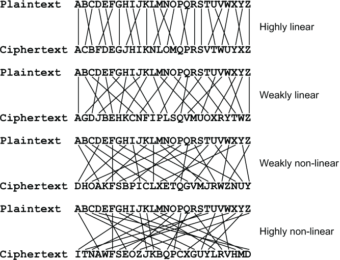
There are degrees of linearity and non-linearity. A substitution may be highly linear, weakly linear, weakly non-linear or highly non-linear. One example of each kind should get the point across. I have drawn a line between the position of each letter in the plaintext alphabet and its position in the ciphertext alphabet. You can see right away how much better the mixing of the alphabet becomes as the substitution becomes more non-linear.
In the discussions that follow, I refer to the S-box inputs as the plaintext and the key, and to the output as the ciphertext. These terms mean the plaintext and ciphertext for that individual S-box, and not necessarily the plaintext and ciphertext for the entire multi-round block cipher. In some block ciphers the S-boxes do not have keys, they merely perform a simple substitution. In that case you can imagine that the S-box has a key that has the constant value 0, or that the S-box key is 0 bits long.
It is assumed here that Emily is able to test the S-box(es) for linearity because the cipher has been published, or she has obtained a copy of the device. If all that Emily has available is the input to the first round and the output from the last round, then linearity testing might not be feasible.
12.3.1 Correlation coefficient
There is a well-established statistical method for testing the correlation between two numerical variables. For example, you could test the correlation between daily temperature, measured in degrees Celsius, and sunlight, measured in hours. Temperature and hours are the numerical variables. You could make multiple trials taking the temperature at some fixed time of day, and recording the hours of sunlight that day. This would give you two lists of numbers, one list for the temperature and a corresponding list for the sunlight hours. The statistic measures the correlation between these two lists of numbers.
In our case the two variables are the plaintext letters and the ciphertext letters. The “trials” are the positions in the alphabet. For example, the first trial could be “A” and the last trial could be “Z”. The letters of the alphabet need to be numbered in some manner. The numbering will depend on the size of the alphabet. For example, a 27-letter alphabet could be numbered using 3 ternary (base-3) digits as we did for the trifid cipher in section 9.9. The correlation could be between any ternary digit of the plaintext letters and any ternary digit of the ciphertext letters. In the following two sections I will discuss this in detail for the 26-letter alphabet and the 256-character alphabet.
Linearity is measured by calculating the correlation between the two variables. By far the most widely used measure of correlation is the Pearson product-moment correlation coefficient developed by English mathematician Karl Pearson, the founder of biometrics, and published in 1895, although the formula itself had been published in 1844 by French physicist Auguste Bravais, who was known for his work in crystallography. The purpose of the correlation coefficient is to have a single number that tells how well two variables are correlated, a number that has the same meaning regardless of the units of measurement or the sizes of the numbers involved.
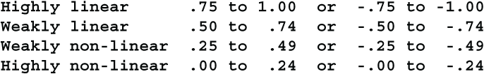
If the two variables have a linear relationship the correlation is 1. If the variables have no correlation whatsoever the correlation is 0. If the two have an inverse relationship the correlation is -1. For example, the number of heads in 20 flips of a coin will have an inverse relationship to the number of tails. A correlation of .8 indicates a strong linear relationship, while a correlation of .2 indicates the relationship is highly non-linear.
Instead of merely presenting the formula, as most textbooks do, I am going to explain how and why it works. Understanding how it works will help you to use it appropriately and correctly.
The goal here is to compare two variables. This is done by comparing the sequence of values over the set of trials. For example, we might want to compare the price of magic carpets sold at the Qeisarieh bazaar in Isfahan, Persia, with their size. There are many factors affecting the price of magic carpets, including the type of yarn, the density of the knots, the complexity of the design and, of course, airspeed.
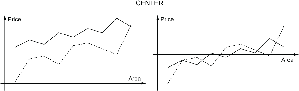
The first step in comparing the variables is to put them side by side, just as you would do if you were comparing them by sight. To put that a different way, you want to eliminate the +x term in the linear relationship P = mA+x, where P is price and A is area. It might seem like you could take the differences Pi-Ai and then subtract the mean difference from P. However, this does not make sense because P and A are in different units. Carpet area A is measured in square arsani (roughly one meter), while carpet prices P in the bazaar are denominated in toman (Persian currency).
You need to adjust the area figures and the price figures separately because they are in different units. The trick is to take the mean price and subtract that from all the price figures to get new, adjusted price figures P'. You calculate the mean price μP by adding up the carpet prices and dividing by the number of carpets. For example, if the prices were 1000, 1200 and 1700 toman you would add up the 3 prices 1000+1200+1700 and divide by 3 to get the mean price of 1300. You would subtract 1300 from each of the prices to get the adjusted prices -300, -100 and 400. As you can see, the adjusted prices P' add up to 0. In a sense, the adjusted prices are centered around 0.
The area figures are centered in the same way. You add up the areas and divide by the number of carpets to get the mean area. For example, if the areas were 10, 12 and 17 square arsani you would add up the 3 areas 10+12+17 and divide by 3 to get the mean area of 13. You would then subtract 13 from each of the areas to get the adjusted areas -3, -1 and 4. The adjusted areas A' also add up to 0. The adjusted areas and adjusted prices are now both centered around 0. They are side by side and ready for the comparison.
The next step is to get the prices and the areas on the same scale. The prices are in toman, the areas are in square arsani, and there is no such thing as a conversion from toman to square arsani. That would be like a conversion from bushels to Celsius. Pearson, or rather Bravais, used an idea from linear algebra called normalization.
Suppose that you have a vector (a,b) and you want to find a vector pointing in the same direction, but whose length is 1. Any multiple of the vector (a,b), such as (ma,mb), will point in the same direction. Multiplying a vector changes its length, but not its direction. If you divide the vector by its length, the new vector (a/L,b/L) will have a length of 1 and the same direction as the original. This also clears the units. Imagine that the length of the vector is measured in feet. If you divide the vector by its length, then you have feet divided by feet. The result is just a number, with no units. It is dimensionless. The same is true when the vector is measured in toman or square arsani.
The length of the vector can easily be found by using the Pythagorean Theorem, L = √(a2 + b2). This can be extended to any number of dimensions, L = √(a2 + b2 + c2 + ...). Let’s try an example to see if this works. Try the vector (3,4). The length of this vector is √(32 + 42) = √(9 + 16) = √25 = 5. The normalized vector is (3/5,4/5). Therefore √((3/5)2 + (4/5)2) = √(9/25 + 16/25) = √25/25 = 1 is the length of the normalized vector, as expected. It worked.
P, A, P' and A' are all lists of numbers, so they are vectors. They have lengths just like any vector, and they can be normalized like any vector. In geometry, a vector is normalized by dividing it by its length. The length of any normalized vector is always 1.
To normalize P' you just square all of the adjusted prices, add those squares and take the square root of the sum. That gives you the length of P'. Divide the adjusted prices P' by the length to get the normalized prices P''. To normalize A' you square all of the adjusted areas, add those squares and take the square root of the sum. That gives you the length of A'. Divide all of the adjusted areas A' by the length to get the normalized areas A''.
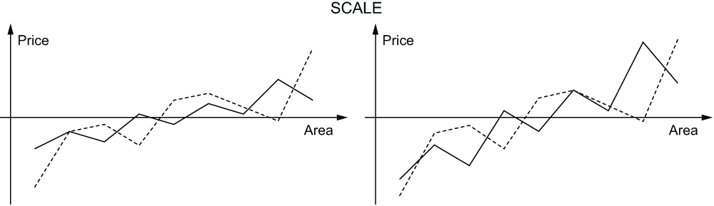
To recap, (1) center the prices and areas by subtracting the mean, then (2) normalize the prices and areas by dividing by the length. The result is a standardized list of prices and a standardized list of areas where the sum of the terms in each list is 0, and the sum of the squares of the terms in each list is 1.
Now we are all set up for the formula. Multiply each term in the normalized list of prices by the corresponding term in the normalized list of areas, so P''i×A''i. Add up those products. That’s the correlation coefficient. (In linear algebra this is called the inner product, or dot product, of the normalized price vector and the normalized area vector.)
Let’s give this a reality check. Imagine we are testing the correlation between Celsius temperature and Fahrenheit temperature. We know these are related by the linear formula F = 1.8C+32, so the correlation coefficient ought to be 1. Suppose we measure the temperature at 11AM, 3PM, 7PM and 11PM, and find that the Celsius temperatures are (14, 24, 6, 0) and the Fahrenheit temperatures are (57.2, 75.2, 42.8, 32). The mean Celsius temperature is (14+24+6+0)/4 = 11, so the adjusted Celsius temperatures C' are (3, 13, -5, -11), and the corresponding adjusted Fahrenheit temperatures F' are (5.4, 23.4, -9, -19.8). The length of the Celsius C' vector is 18. Divide C' by 18 to get C'', the normalized Celsius temperatures (3/18, 13/18, -5/18, -11/18). The length of the adjusted Fahrenheit vector F' is 32.4 and the normalized Fahrenheit vector F'' is (3/18, 13/18, -5/18, -11/18).
We multiply C'' by F'' element by element and add the 4 products to get the correlation coefficient. This sum is (3/18)2+(13/18)2+(-5/18)2+(-11/18)2. It all adds up to 1. This supports the claim that the procedure described previously, centering by subtracting the mean, normalizing by dividing by the length, and then multiplying term by term and summing, does indeed produce a valid correlation coefficient.
To recap: you test for linearity by calculating the correlation coefficient. This section has shown you how to calculate the correlation coefficient. The calculation yields a number between -1 and +1. Here is a chart for interpreting the correlation coefficient.
12.3.2 Base-26 linearity
Let’s start the investigation of linearity with substitutions based on a 26-character alphabet. This might be valuable if you are designing a mechanical or electromechanical cipher device, or if you are simulating one. Each rotor in such a machine performs a substitution on a 26-character alphabet. Begin by considering an S-box that has no key. There are multiple forms of linearity that can occur with a 26-letter alphabet, depending on how the letters are numbered. There are 3 ways to view the alphabet: treating the alphabet as a single sequence of 26 letters, treating it as a 2×13 array of letters, or treating it as a 13×2 array of letters. These lead to 3 different ways of numbering the characters: N1, N2 and N3, as shown. The discussion of these 3 numbering schemes uses modular arithmetic. If you would like to review modular arithmetic at this time, see section 3.6.

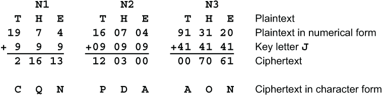
Numbering schemes N2 and N3 follow the usual convention of using the letters A, B and C to represent digits beyond 9. That is, they use the first 13 of the 16 hexadecimal digits. In the simplest linear encipherment (the Belaso cipher) the key is just added to the plaintext. When the key is added to the plaintext character, in the N1 numbering scheme it uses conventional addition modulo 26. When the key is added to the plaintext character in the N2 numbering scheme, the first digit is added modulo 2 and the second digit is added modulo 13. Conversely, when the key is added to the plaintext character in the N3 numbering scheme, the first digit is added modulo 13 and the second digit is added modulo 2. Here are examples showing how the word THE is enciphered by adding the key J in each of the 3 schemes.
If the plaintext, the key and the ciphertext alphabets are all numbered using the N1 scheme, then a linear substitution, or linear transformation, would take the plaintext character p and transform it using the key k into the ciphertext character c = mp+f(k), where m is a multiplier which must be coprime to 26, f(k) is any integer-valued function, and the arithmetic is done modulo 26. For example, if m = 5, p = 10, k = 3 and f(k) = k2+6, then c = 13 because 5×10+32+6 = 65≡13 (mod 26). The constant m and the function f(k) can be built into the substitution table.
If the plaintext, the key and the ciphertext alphabets are all numbered using the N2, or 2×13 numbering scheme, either the first digit or the second digit or both digits can be linear. Suppose that both digits are linear. Then a plaintext character p = a,b is transformed using the key k into the ciphertext character c = ma+f(k),nb+g(k), where m must be coprime to 2, meaning m = 1, n must be coprime to 13, and f(k) and g(k) may be any integer-valued functions. The arithmetic is done modulo 2 and modulo 13, respectively. The constants m and n, and the functions f(k) and g(k) can be built into the substitution table.
If the plaintext, the key and the ciphertext alphabets are all numbered using the N3, or 13×2 numbering scheme, either the first digit or the second digit or both digits can be linear. Suppose that both digits are linear. Then a plaintext character p = a,b is transformed using the key k into the ciphertext character c = ma+f(k),nb+g(k), where m must be coprime to 13, n must be coprime to 2, meaning n = 1, and f(k) and g(k) may be any integer-valued functions. The arithmetic is done modulo 13 and modulo 2, respectively. The constants m and n, and the functions f(k) and g(k), can be built into the substitution table.
There is no requirement that the plaintext and the ciphertext are numbered the same way. There can be a correlation between any digit of the plaintext and any digit of the ciphertext in any numbering. Emily might test any or all of these combinations, looking for an exploitable weakness. Consequently the designer of the cipher must test all of the possible numberings and correlations to verify that no such weakness exists, or to learn where countermeasures must be taken to prevent Emily from exploiting such a weakness. For example, you can use substitutions that have different weaknesses in alternating rounds of a block cipher. In most cases each substitution will diminish the weakness of the other. Of course, you should test this by hunting for linear relationships between the plaintext and the final ciphertext produced by the last round.
If you wish to test the linearity of a substitution, you cannot apply the correlation coefficient directly. This is because all of these substitutions are done using modular arithmetic. Consider this substitution using the N1 numbering scheme:
![]()
This is almost exactly c = 2p, so it is highly linear. However, the correlation coefficient between the plaintext and the ciphertext alphabets using this numbering scheme is .55556, indicating that the substitution is only weakly linear. The correlation coefficient should have been calculated using the following distribution, which is equivalent modulo 26.
![]()
The correlation coefficient using this numbering is .99987, correctly showing very strong linearity.
This illustrates a difficulty of using the correlation coefficient in cryptography. You are always working modulo the size of the alphabet. To find the correct correlation you need to add 26, then 52, 78 and so forth for the N1 numbering, or 13, 26, 39, ... for the N2 and N3 numberings. In the previous example the place where you needed to start adding 26 was obvious. It was where the ciphertext numbering went 22 24 1 3. That drop from 24 down to 1 made it apparent.
When the ciphertext alphabet is less linear, when it jumps around a bit, it may be harder to spot. For example, this substitution has a correlation of .3265, moderately non-linear.

When it is adjusted by adding multiples of 26 like this

the correlation becomes .9944, highly linear. I have used single, double and ![]() underlining to show where 26, 52 and
underlining to show where 26, 52 and ![]() , respectively, have been added to the ciphertext characters. An important feature to notice here is that 26 was added to the ciphertext character 2, corresponding to plaintext 5, but not to the following ciphertext characters, 21 and 25. Likewise, 52 was added to the ciphertext character 1, corresponding to plaintext 14, but not to the following ciphertext character, 24.
, respectively, have been added to the ciphertext characters. An important feature to notice here is that 26 was added to the ciphertext character 2, corresponding to plaintext 5, but not to the following ciphertext characters, 21 and 25. Likewise, 52 was added to the ciphertext character 1, corresponding to plaintext 14, but not to the following ciphertext character, 24.
It is fairly easy to determine which multiple of 26 to add when the ciphertext alphabet is close to linear. When the ciphertext alphabet is badly behaved it becomes much harder. But ... that doesn’t matter. When the substitution is non-linear, that is all you need to know. It makes no difference if the correlation coefficient is .01 or .35. In either case there is not enough correlation for Emily to exploit. Don’t waste time calculating the exact value.
That handles the case with no key. Now suppose there is a key. If the substitution is linear, then it will have the form d(p)+f(k), where p is the plaintext, k is the key and d and f are integer-valued functions. The addition can be done in any of the 3 numbering schemes, N1, N2 or N3. In this case the key plays no role in testing the linearity. f(k) is just a constant added to the ciphertext. Adding a constant has no effect on the correlation coefficient because it just gets subtracted back out when you subtract the mean value from each list of values (the centering operation). It is easy to test whether the substitution S(k,p) takes the form d(p)+f(k). Just choose two keys k1 and k2 and take the differences S(k1,0)-S(k2,0), S(k1,1)-S(k2,1), S(k1,2)-S(k2,2), ... If the S-box has the form d(p)+f(k), then all of these differences will be equal. If you repeat that for all possible keys, then you are certain S(k,p) has the desired form, and you can test for linearity without considering the key.
12.3.3 Base-256 linearity
This analysis of linearity in base 26 is just a warmup for base-256 linearity because there are two distinct forms of linearity that can occur in base 256. Let’s call them serial and condensed. In serial linearity each group of bits represents an integer. For example, the 3-bit groups 000, 001, 010, ... , 111 represent the numbers 0, 1, 2, ... , 7. The two forms of linearity can be combined to make a hybrid form of linearity. This is discussed later in section 12.3.6.
Serial linearity is what we saw with base 26. In base 26, there could be correlations between the N1, N2 and N3 numberings in any combination and in any order, so there were many pairings that had to be tested for linearity. In base 256 there are more possibilities. Serial linearity may exist between any group of bits in the plaintext alphabet and/or the key versus any group of bits in the ciphertext alphabet. These bit groups need not be the same size. A 4-bit group taken from the plaintext, covering the range from 0 to 15, may be highly correlated with a 3-bit ciphertext group covering the range 0 to 7, so the number of possible pairings is much greater.
To make matters worse, the 4 bits in that 4-bit group could be any bits from the plaintext byte. Bits 7,2,5,1 in that order are just as valid as bits 1,2,3,4. The linear substitution might add these 4 bits to 4 different bits of the key byte modulo 16. The number of possible combinations becomes enormous. To recap, any group of bits in any order in the plaintext character plus key character can be linearly correlated with any group of bits in any order in the ciphertext character. That’s a boatload of correlations to test.
Before you reach for the Excedrin, or the tequila, here is some good news. You probably don’t need to test for any of them. Unless the cipher is specifically designed to pass these values intact from round to round, these correlations won’t matter. They will get so weakened with each successive round that they won’t be detectable from the initial plaintext through the last round of the block cipher.
12.3.4 Adding a backdoor
You may have noticed that I said “probably.” The exception is when you suspect that a cipher may have a backdoor, that is, it has been deliberately designed so that people who know the secret can read messages without knowing the key. For example, a national espionage agency might supply its agents with a cipher that has a backdoor so that the agency can monitor their messages and detect traitors.
At this point, let’s change hats. Suppose that you are Z, the spymaster who has been tasked with designing this cipher. You need to build a cipher that looks and acts like a strong block cipher, so the users will not suspect a thing. For example, you would want your cipher to have the Fifty-Fifty property, where changing just one bit in the key or the plaintext would cause about half of the ciphertext bits to change in a random-looking pattern. If the substitutions in your block cipher were not all linear, this would be a sure sign of a strong block cipher. You want your fake cipher to mimic that property.
Here is one method you can use to hide a backdoor in a cipher. It is based on serial linearity, so let’s call it the Backdoor Serial method for constructing a cipher, and let’s call ciphers constructed by this method Backdoor Serial ciphers. Z can read messages that are sent using backdoor serial ciphers without needing to know the key, but for anyone who does not know how the backdoor works, they look like strong, secure block ciphers. The method has three parts: disguise, concealment and camouflage.
The backdoor serial ciphers will use linear substitutions on hex digits. Each block of the plaintext and the key is treated as a sequence of 4-bit hexadecimal digits. The enciphering operation is addition modulo 16 on the hex digits of the message block and the key. Suppose the two hex digits in a byte are p1 and p2, and the hex digits of the key that is used to encipher them are k1 and k2. The linear substitution will replace p1 and p2 by
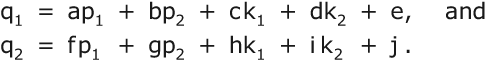
The coefficients a, b, c, d, e, f, g, h, i and j may be any integers from 0 to 15, and ag-fb must be odd. If your cipher has multiple rounds, these 10 values may be different for every round.
This type of linear substitution is easy for Emily to detect. In particular, the low-order bit of each hex digit is purely linear, so a simple bit-to-bit test for linearity will find it. To avoid detection, we can disguise the hex digits. First, list the hex digits in some scrambled order, like this:

To add two disguised hex digits, you add their positions in the scrambled list to get the position of the sum in the scrambled list. For example, to add 1+2, you find that the digit 1 is in position 9 and the digit 2 is in position F, so you add 9+F mod 16 to get 8. The sum is in position 8 in the list. The digit in position 8 is D, so 1+2 = D.
Likewise, to multiply two disguised hex digits, you multiply their positions in the scrambled list to get the position of the product in the scrambled list. For example, to multiply 2×3 you note that the digit 2 is in position F and the digit 3 is in position 2, so you multiply F×2 mod 16 to get E. The product is in position E in the list. The digit in position E is 7, so 2×3 = 7.
Essentially the disguise is a simple substitution done on the hex digits. If the substitution is non-linear, then none of the bits will have a linear relationship between the plaintext and the ciphertext. This type of disguised linearity is much harder for Emily to detect, but to really confound Emily you can conceal the disguised hex digits.
If the hex digits are always bits 1-4 and bits 5-8 of each byte of the block and key, then Emily still stands a chance of discovering the linearity. To really make Emily’s task seriously hard, you can conceal the bits within each byte. Instead of using bits (1,2,3,4) of the plaintext, and bits (1,2,3,4) of the key, and putting the resulting sum in bits (1,2,3,4) of the ciphertext, you could take the hex digits from bits (2,7,4,1) of the plaintext, in that order, and bits (4,8,3,5) of the key, and put the resulting sum into bits (8,6,1,7) of the ciphertext byte. You can use any combination of 4 bits that you choose, in any order, as long as the 2 hex digits in each byte use all 8 bits once each.
Just to be clear, we are not saying that Sandra extracts these bits from each byte, deciphers the disguised linear substitution, performs the arithmetic, then repacks the resulting bits in a different order. That would be far too slow, and Emily would know exactly what was afoot. Instead, Sandra does this when she builds the substitution tableau. To encipher, she simply uses the key byte to select a row in the tableau and then performs the substitution on the plaintext byte. All of the disguise and concealment are built into the substitution tableau.
The cipher, as described so far, is merely a very complicated polyalphabetic cipher. Emily could solve messages using the techniques of section 5.8.3. To make a backdoor serial cipher look like a strong block cipher, you need some camouflage to hide the polyalphabetic cipher that is at its core.
One method is to use a bit transposition that is applied to the block after each round. This will make the cipher look like a substitution-permutation network (section 11.1). To preserve the hidden linearity, the 4 bits that make up each hex digit must end up in a single byte. They need not be in the same bit positions in that byte, and they need not be contiguous, but they must be in one byte together. In other words, each byte of the input gets split into two hex digits that are fed into two other bytes at the next round in some transposed order. Unfortunately, if Emily has access to the published specifications for the backdoor serial cipher, she might well discover this type of camouflage.
Let’s look at a second form of camouflage that is much harder for Emily to uncover. This method borrows an idea from the Data Encryption Standard (DES) (section 11.2). Each cipher block is divided into two halves. In each round, first the left half is used as the keys to encipher the right half, then the right half is used as the keys to encipher the left half. We have already seen how the linearity can be disguised and concealed within the substitution tableau, so let’s take advantage of that to create the illusion of a strong block cipher.
Each round of the cipher will consist of four steps. (1) Each byte in the left half is enciphered using one byte of the key. (2) Each byte of the right half is enciphered using one byte of the left half as the key. (3) Each byte in the right half is enciphered using one byte of the key. (4) Each byte of the left half is enciphered using one byte of the right half as the key.
To make this look ultrastrong, each byte of the block should be enciphered using a different byte of the key in each round, and each byte of one half of the block should be enciphered using a different byte from the opposite half in each round. You can fancy this up by shuffling the bytes in the block and the bytes in the key for every round. You can make the key larger than the block to present an even greater impression of strength. The cipher remains linear, however, because the linearity has been preserved in every step of every round.
Let’s look at the mechanics of the backdoor serial cipher. In each byte of the key, the plaintext and the ciphertext there are two hex digits. Each of these could occupy any 4 bits of the byte, in any order. Let’s call that ordered set of 4 bits the bit configuration of the hex digit, and the combination of 2 hex digits in a byte the byte configuration. The key does not normally change configuration, but the byte configuration of the plaintext and ciphertext can change at any stage of the encipherment.
For each substitution there are 6 bit configurations, 2 for the key, 2 for the plaintext and 2 for the ciphertext. For each hex digit, the permutation (scrambled order) of the 16 hex values also can be different, so there are also 6 permutations of the hex values for each substitution, 2 for the key, 2 for the plaintext and 2 for the ciphertext. This combination of 6 configurations and 6 permutations determines the substitution tableau. For each distinct combination of bit configurations and permutations a separate substitution tableau is needed.
Each tableau uses 65,536 bytes, so storage might be a problem. If this is an issue, I suggest using at most 2 byte configurations, and for each bit configuration using at most 2 different permutations, perhaps alternating from one round to the next. To further reduce the amount of storage required, you could consider using the same permutation each time you use any given bit configuration.
12.3.5 Condensed linearity
In most cases, you will not be building a backdoor into your cipher, and you will not be concerned with serial linearity. Let’s turn our attention to the second type of linearity, condensed linearity. In this form of linearity, a group of bits is condensed down to a single bit by exclusive-ORing them together. Thus 000, 011, 101 or 110 would be condensed to 0, while 001, 010, 100 or 111 would be condensed to 1. Any group of bits from the plaintext and/or the key could potentially be correlated with any group of bits from the ciphertext for each S-box. If a block cipher uses exclusive-OR to combine the outputs of the S-boxes with the rest of the block, then this linearity can be passed from round to round, and there will be a linear relationship between the original first-round plaintext and the final last-round ciphertext. The designer of the cipher must either avoid using exclusive-OR this way, or must make a thorough check to be certain that the S-boxes do not contain any such linearities.
Suppose the S-box takes an 8-bit plaintext and produces an 8-bit ciphertext. There are 255 different ways a group of bits can be selected from the plaintext and likewise 255 ways a bit group can be selected from the ciphertext. (The order of the bits does not matter since a⊕b = b⊕a.) That makes 2552 = 65,025 different pairings of groups to test. Each test is a correlation between the 256 plaintext values and the 256 ciphertext values. This is easily feasible, even on a personal computer.
If the S-box takes an 8-bit plaintext plus an 8-bit key and produces an 8-bit ciphertext, then there are 65,535 different ways a group of bits can be selected from the plaintext plus key, and again 255 ways a bit group can be selected from the ciphertext. That makes 65,535×255 = 16,711,425 different pairings to test. This takes a good while on a PC because each correlation involves all 65,536 plaintext and key combinations. That’s over 1012 values that need to be centered, scaled and summed.
This is the ideal time to talk about how to do these tests efficiently. There are a few tricks that greatly speed up the process. (1) To select a combination of bits, use a mask that selects those bits from each byte. For example, if you want bits 2, 4, and 7, use the mask 01010010, which has ones in bit positions 2, 4 and 7. AND this mask with each plaintext byte to select the desired bits. (2) To try all of the possible bit combinations, don’t construct the masks one at a time, just step the mask through all of the values 1 through 255. (3) To condense the bits, don’t use shift and XOR every time. Do that once and build a table of the condensed values. Then a bit combination can be condensed by a table lookup. If there is a combination of key bits and plaintext bits, these can be exclusive-ORed together and the result can be condensed using the table, so you will need one table lookup instead of two.
12.3.6 Hybrid linearity
For the sake of completeness, I will mention that it is possible to have a hybrid form of linearity that combines serial and condensed linearity. Suppose that you divide each 8-bit byte into four 2-bit groups. These 2-bit groups could be serially linear under addition modulo 4. You could condense two or more of these groups by adding them modulo 4. The same could be done with 3-bit groups modulo 8 or 4-bit groups modulo 16.
Let’s stick with 2-bit groups. Each group could consist of 2 bits taken from anywhere in the byte. For example, a byte could be decomposed into 4 groups, bits (6,1), (4,8), (2,5) and (7,3). You can condense several 2-bit groups into a single 2-bit group by adding them modulo 4, or by taking any linear combination modulo 4. For instance, if the 2-bit groups are A, B, C and D you could combine them into a new 2-bit group pA+qB+rC+sD+t (mod 4), where p, q, r, s and t are fixed integers in the range 0 to 3, with at least one of p, q, r and s being odd.
These types of condensed groups could be correlated with similar hybrid groups of bits in the ciphertext, or with regular bit groups or condensed bit groups from the ciphertext. If you want to be absolutely thorough, then all of the possible pairings of linear groups, condensed groups and hybrid groups need to be tested for correlation.
12.3.7 Constructing an S-box
Here are three methods for constructing an S-box with good non-linearity properties: the Clock Method, SkipMix and the Meld8 Method.
On a sheet of paper, arrange the letters of the alphabet evenly spaced clockwise around a large circle like the numerals on a clock face. Choose a starting letter and a second letter and draw a straight line from the first to the second. Then choose a third letter and draw a straight line from the second letter to the third letter, and so forth. Define the span of each line to be the number of letter positions you move forward in a clockwise direction from each letter to the next. For example, using the 26-letter alphabet, the span from C to D is 1, and the span from D to C is 25. To make the substitution as non-linear as possible, make each span a different length.
Here is how it can be done. For each letter of the alphabet, make a list of all the letters that can possibly follow it. When you begin, the list for each letter will contain every other letter, so you would have 26 lists of 25 letters apiece. Each time you choose a letter and add it to the mixed alphabet, delete that letter from all of the lists. If the span from the previous letter to that letter is s, then also delete any other letter whose span is s from all of the lists. For example, suppose you have added P and then R to the alphabet. The span from P to R is 2 positions, PQR. Therefore, in the A list you would delete C, in the B list you would delete D, in the C list you would delete E, and so forth.
Eventually some lists become empty. If there is only one letter whose list is empty, then that letter will have to be the last letter in your mixed alphabet. If there are two lists that are empty, then you have hit a dead end. Start over, or backtrack and try again. Each time you choose the next letter to add to the alphabet, choose a letter that has a short list, but not one with an empty list, unless that’s the last letter left.
Here is an example of an alphabet constructed by the clock method:
![]()
There are 5 different numberings that need to be tested to check the linearity of this alphabet: the N1 numbering, the first and second digits of the N2 numbering, and the first and second digits of the N3 numbering. Each of these must be correlated with the same 5 numberings for the standard Latin alphabet, making 25 correlations in total. You want all of the correlations to be between -.5 and +.5. Even better would be to have them all between -.333 and +.333.
Here are the results of those tests, the 25 correlation coefficients.
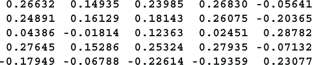
As you can see, all of the correlations are between -.226 and +.288, with 6 of them falling between -.1 and +.1, so the clock method is an excellent method for constructing non-linear substitutions.
There is no guarantee that you will get such good results every time. You still need to test for linearity.
Earlier in this section (12.3) I mentioned that an alphabet could be constructed using the SkipMix algorithm (section 5.2) with a pseudorandom number generator. In general, choosing an alphabet at random does not lead to good non-linearity properties, so let me describe the best way to use SkipMix in more detail. This time I will illustrate with a 256-character alphabet.
As always, you begin by listing the 256 available characters. Generate a random number in the range 1 to 256 to select the first character. Suppose that is position 54 in the alphabet. Take that character and then delete it from the list. Now there are 255 characters left. Generate a random number in the range 1 to 255. Suppose that number is 231. The next position would be 54+231 = 285. Since that is greater than 255, you subtract 255 to get 30. Take the next character from position 30, and delete it from the list. You have now taken 2 characters, and there are 254 characters left, so you generate a random number in the range 1 to 254. And so forth.
The resulting alphabet has good non-linearity properties because you generate the random number in a different range each time. This is loosely analogous to making all of the spans different in the clock method. Here is an example of a 26-letter alphabet generated by this version of SkipMix.
![]()
This can be tested the same way as the clock alphabet. The results are
These results are good. All of the correlations lie between -.127 and +.344, with 5 of them falling between -.1 and +.1, however, they are not as good as the clock method results.
This method is basically a special-purpose pseudorandom number generator. I will assume that the computer language you are using is able to operate with 64-bit integers. Depending on the way large integers are represented, you may be able to handle integers up to 262 or 263. To be cautious, I will assume 262. The first step is to choose two numbers, a multiplier m of 24 to 26 bits, and a modulus N of 35 to 37 bits. The modulus must be a prime. It is best if m is a primitive root of N, however, since I have not explained what that is yet, just make both m and N prime.
Test your choices of m and N by multiplying them together. If the result is greater than 262, or about 4.611×10¹⁸, then make either m or N smaller.
To generate the random numbers, start with any integer s between 2 and N-1 as the seed. Multiply the seed by m and reduce it modulo N to get the first pseudorandom number. Multiply the first random number by m and reduce it modulo N to get the second random number, and so forth. That gives you a sequence of random numbers in the range 1 to N-1. You will use those random numbers to generate the alphabet.
Suppose N has 36 bits. Number the bits of N from 1 to 36 starting at the high-order end. Take the first 8 bits of each random number, bits 1 to 8. Delete them from the high-order end, and exclusive-OR them with the next 8 bits, bits 9 to 16. This is the Meld8 operation. Its purpose is to make the sequence of characters non-linear. Here is an example:
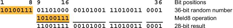
The next step is to use the 28-bit random number to generate a character. This depends on whether you are building a 26-character or a 256-character alphabet. For a 26-character alphabet, multiply this number by 26 and divide by 228 (or shift right 28 places) to get the next character. For a 256-character alphabet, just divide by 220, or shift right 20 places to get the next character.
Start with an empty alphabet and add one character at a time. If this is a new character, you append it to the alphabet. If this is a duplicate, you discard it. Since you are not taking consecutive random numbers, this also works to make the alphabet non-linear. Here is an example of such an alphabet generated with the modulus N = 90392754973, the multiplier m = 23165801 and the seed s = 217934:
![]()
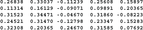
The resulting correlation coefficients are
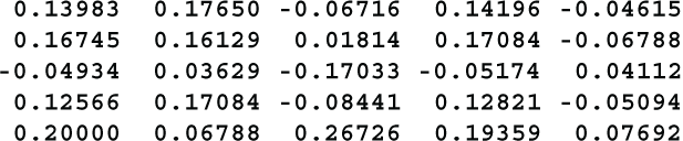
The correlations range from -.170 to +.267 with 11 of them falling between -.1 and +.1. This is the best of the three examples, however, it would be folly to conclude that Meld8 was the best method based on a single example of each technique. Always test.
12.3.8 S-box with a key
In section 12.3.7 we dealt with S-boxes that had no key. They performed a simple substitution. When a key is used, the S-box performs a general polyalphabetic substitution (section 5.8.3). The S-box can be considered a tableau, with each row being one mixed alphabet. The S-box can be generated by constructing each of these mixed alphabets using the clock method, SkipMix or Meld8, or by any combination of methods.
If you use the clock method or SkipMix, use a different random seed each time. If you use Meld8, it is acceptable to use the same modulus each time, but use a different seed and a different multiplier. As always, test, test, test. Your objective is to avoid any linear relationship between the combination of the key and the plaintext with the ciphertext. If the results are subpar, meaning that a lot of the correlation coefficients are outside the range -.35 to +.35, it might take no more than replacing one row or swapping two rows of the tableau to fix the problem.
12.4 Diffusion
Shannon’s second property is diffusion. The idea is that every bit or byte of the ciphertext should depend on every bit or byte of both the plaintext and the key.
To illustrate this, let’s go back to Delastelle’s bifid cipher, described in section 9.6. To refresh your memory, the bifid is a block cipher based on a Polybius square. If the block size is S, then each letter of the message is replaced by two base-5 digits and the digits are written vertically into a 2×S grid and read out horizontally. Then the pairs of digits are turned back into letters using the same or a different Polybius square.
Let the block size be 7, and call the letters in the plaintext block A,B,C,D,E,F,G. Let the digits representing these letters be aa,bb,cc,dd,ee,ff,gg. I have left off the subscripts because it does not matter here which digit is first and which digit is second. The block will then be
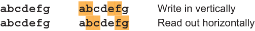
When the letters are read out of the block horizontally you get ab,cd,ef,ga,bc,de,fg. Notice that each letter of the ciphertext depends on two letters of the plaintext. The first ciphertext letter depends on A and B, the second letter depends on C and D, and so forth.
At this point I need to introduce a special notation to show which plaintext letters each ciphertext letter depends on. If a ciphertext letter depends on plaintext letters P, Q and R it gets designated pqr. Using this notation, if you enciphered the letters A,B,C,D,E,F,G a second time, the block would look like this:
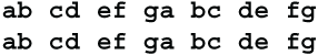
Reading these letters out horizontally you get abcd, efga, bcde, fgab, cdef, gabc, defg. Since the order of the digits is irrelevant, this could also be given as abcd, aefg, bcde, abfg, cdef, abcg, defg. After two encipherments, each ciphertext letter depends on four plaintext letters.
If you encipher this block a third time using the bifid cipher, every ciphertext letter will depend on all 7 of the plaintext characters. For the bifid cipher with block size 7, three rounds of encipherment are required to get full diffusion. If the block size were 9, 11, 13 or 15, four rounds of encipherment would be needed. (Recall that the block size in a bifid cipher should always be odd.)
In general, to test diffusion you begin with each plaintext character or bit depending on just itself. If the cipher operates on whole bytes or characters, you trace diffusion on the basis of bytes. If it operates on hexadecimal digits, digits in some other base, or individual bits, you trace the diffusion on the basis of those units. For the bifid cipher, the units are the Polybius square coordinates, or base-5 digits.
To track the diffusion, you need a way to represent the set of plaintext units and key units as they trickle through the rounds of the block cipher. When there are just a few plaintext units, as there were for the bifid example, it works well just to list them. When the number of plaintext, key and ciphertext units is larger, a more compact representation may be necessary. A good strategy is to make a binary vector for each ciphertext unit. Let’s call this a dependency vector. Each element of the dependency vector will correspond to one input, either a plaintext or key unit. The dependency element will have the value 1 if the ciphertext unit depends on that input unit, and 0 otherwise.
When two or more input units are combined to form an output unit, their dependency vectors are ORed together to form the dependency vector for the output unit. To illustrate how this works, let’s go through the bifid example again using this notation. Initially each character depends only on itself. This is represented by the vectors
![]()
After the first application of the bifid cipher, each resulting letter depends on two of the plaintext letters. The first round 1 output byte depends on the first two round 1 input bytes, so you OR their dependency vectors together 1000000∨0100000 to get 1100000. The second output letter depends on the third and fourth plaintext letters, so you OR their dependency vectors together 0010000∨0001000 to get 0011000, and so forth. The output of the first round is represented by the vectors
![]()
After the second round of bifid, the first output letter depends on the first and second outputs from the first round, so you OR their dependency vectors together 1100000∨0011000 to get 1111000. The second output letter depends on the third and fourth outputs from the first round, so you OR their dependency vectors together 0000110∨1000001 to get 1000111, and so on. After two rounds of bifid each letter depends on four plaintext letters, represented as
![]()
After the third round of bifid, each output letter depends on all 7 of the round 1 plaintext letters, for example, 1111000∨1000111 is 1111111. The output of the third round is represented as
![]()
Any time an S-box is encountered, the dependency vectors for the output units are formed by ORing together the vectors for each input that contributes to that output. Let’s look at some other situations that may occur in a block cipher.
If two units are exclusive-ORed together, the dependency vector for the output unit is formed by ORing together the vectors for each input. The same is done when several units are combined using any combining function, such as sxor or madd.
When the units of a block are transposed using a key, each output unit is then dependent on all of the units of that key, so the vectors for the key are ORed with the vector for each output unit.
Suppose an S-box is created by mixing its alphabet using a key. If the S-box is fixed or static, say by embedding it in hardware, then the mixing key is no longer involved. If the S-box is variable, perhaps mixed using a different key for each encryption, then the output units of that S-box are dependent on all of the units of that key. The vectors for the key are ORed with the vector for each output unit.
It is possible to express diffusion as a single number. Form a matrix from the dependency vectors for all of the output units. Each row in the matrix will represent one output unit from the final round of the block cipher. Each column in the matrix will represent one input unit, either key or plaintext. The measure of diffusion, or diffusion index, is the portion of these elements in this matrix that are 1. If the matrix elements are all 1, then there is complete diffusion and the diffusion index is 1. If the S-boxes are non-linear and the key is long, this is an indication that the block cipher is strong.
Diffusion is not the full story. There are valid cipher designs where the diffusion index may be less than 1, yet the cipher is strong. One example is a block cipher where there is a separate key for each round. The keys from the early rounds may achieve full diffusion, but the keys from the late rounds, and particularly from the final round, may not. However, if the keys that are fully diffused contain your target number of bits, then the cipher may well be secure, and the partly diffused keys are just insurance.
Here is an example that may help illustrate how the cipher can be strong even when there is less than full diffusion. Consider a cipher with 12 rounds, where each round has an independent 24-bit key. In this cipher it takes 6 rounds to achieve full diffusion, so after 6 rounds the plaintext and the first-round key are fully diffused. After 7 rounds the plaintext and the first- and second-round keys are fully diffused. And so forth. After 12 rounds, the plaintext and the keys for the first 7 rounds are fully diffused. With 24-bit round keys, that is 168 bits of fully diffused keys. If your target strength is 128 key bits, then you have already surpassed your goal. The partially diffused keys from rounds 8 through 12 are a bonus.
12.5 Saturation
Confusion and diffusion are two pillars of the security framework. To make certain that the block cipher is on a firm foundation I propose adding a third pillar, which I call saturation. Diffusion only indicates whether or not a given output unit depends on a given input unit. Saturation measures how much a given output unit depends on a given input unit. I show how to calculate a saturation index analogous to the diffusion index of the preceding section. Saturation is essentially a more refined version of diffusion. With diffusion, the dependency can have a value of only 0 or 1, but with saturation, the dependency can have any non-negative value.
Here is the quick explanation of saturation. Suppose block cipher X consists of several rounds of substitution. In each round, each byte of the message is exclusive-ORed with one byte of the key, and then a simple substitution is done on the result. Suppose that a different byte of the key is used in each round, so that every byte of the key gets used one time for each byte of the block. Cipher X would have little saturation because each byte of the ciphertext depends on each byte of the key only once. To get higher saturation, each output byte would need to depend on each input byte multiple times.
Another example might help make this clearer. Imagine a cipher that operates on a 48-bit block, viewed as six 8-bit bytes. Each round of this cipher consists of two steps: (1) the block is cycled left one bit position, so the leftmost bit moves to the rightmost position, then (2) a simple substitution S is performed on each of the 8 bytes. After the first round, the first output byte C1 depends on the last 7 bits of the first plaintext byte and the first bit of the second plaintext byte, like this:
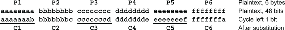
Ciphertext character C1 depends on 7 bits from plaintext byte P1 and 1 bit from plaintext byte P2. It makes sense to say that C1 depends 7/8 on P1 and 1/8 on P2.
Let’s look at the second round. Call the second-round outputs D1 ... D6.
Ciphertext character D1 depends 7/8 on C1 and 1/8 on C2. Here C1 depends 7/8 on P1 and 1/8 on P2, while C2 depends 7/8 on P2 and 1/8 on P3. The only contribution that P1 makes to D1 is from C1. Since D1 depends 7/8 on C1 and C1 depends 7/8 on P1, it is reasonable to say D1 depends 49/64 on P1. For the same reason D1 depends 1/64 on P3. Let’s call these figures saturation coefficients, and call this calculation, when there is a single dependency, the S1 calculation.
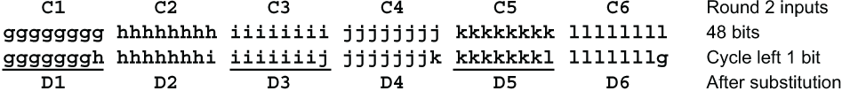
A diagram might make the configuration clearer.
What about P2? D1 gets contributions from P2 via both C1 and C2. It might seem reasonable to say that D1 is 7/8 dependent on C1, which is 1/8 dependent on P2, and 1/8 dependent on C2, which is 7/8 dependent on P2, and conclude that D1 is (7/8)(1/8)+(1/8)(7/8) = 14/64 dependent on P2. That is a reasonable calculation, and it leads to a more sophisticated version of diffusion. However, using that calculation, the total contributions to any given unit will always total 1. The total never grows. If this calculation is repeated many times, all these diffusion figures will converge to 1/48. That is not what the concept of saturation is trying to capture. Saturation should increase whenever a unit receives contributions from several different sources.
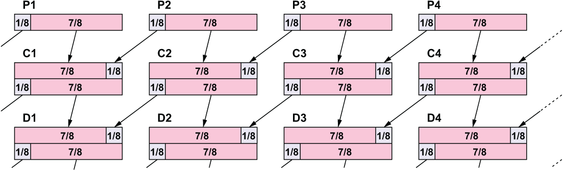
When a unit gets multiple contributions, a different calculation is used to determine the saturation coefficient. Suppose the two sources have saturation coefficients a and b, with a ≥ b. Then the combined saturation coefficient is a+b/2. If there are three contributing saturation coefficients a, b and c, with a ≥ b ≥ c, the combined saturation coefficient is a+b/2+c/4. In each case the component saturation coefficients are sorted in descending order, a ≥ b ≥ c ≥ d ≥ e... . To recap, when multiple saturation coefficients are combined, the results are as follows:
Let’s call this calculation, when there are multiple dependencies, the S2 calculation. Use the S1 calculation for a single source, and use the S2 calculation for multiple sources.
The S2 calculation may seem ad hoc, perhaps even eccentric, but it has just the right properties for a saturation computation. First, it always increases when a unit depends on more than 1 predecessor. This is because a+b/2 is always greater than a. Second, it does not increase too fast. At most, the saturation coefficients can double from one round to the next. This is because a+a/2+a/4+...+a/2n < 2a for any n. For example, 1+1/2+1/4+1/8 = 15/8 = 1.875.
In the present case, D1 depending on P2, the contributing coefficients are 7/8 and 1/8, so the combined coefficient is 7/8+(1/8)/2 = 15/16. The saturation coefficients for an output unit can be formed into a vector, just as the diffusion numbers were. The resulting saturation vector for D1 is thus (49/64, 15/16, 1/64, 0, 0, 0). These vectors can then be formed into a saturation matrix. The saturation index is the smallest coefficient in the saturation matrix.
Let’s look at a more realistic cipher, one that has been proposed in the literature and has probably been used in practice. I will call it SFlip, short for Substitute and Flip. It is a cousin of poly triple flip in section 11.7.5. If you don’t remember what flipping a matrix means, look at section 11.7. The SFlip cipher works on a block of 8 bytes and consists of several rounds plus a finishing step. Each round has two steps. (1) A simple substitution is applied to the eight 8-bit bytes. (2) The 8×8 matrix of bits is flipped. The finishing step is, again, substituting for each of the 8-bit bytes.
The 8×8 matrix of bits requires a 64×64 dependency matrix. This is too large to display legibly, so I will show the cipher in miniature. Let’s use a 3×3 matrix of bits, which has a 9×9 dependency matrix. This cipher will be analyzed twice, once using diffusion, and once using saturation. Diffusion first. Let’s start by labeling the bits in the text block and in the dependency matrix, like so:
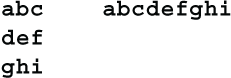
Before the first round each bit depends only on itself, so the dependency matrix looks like (1). After the first-round substitution, each bit is dependent on all 3 bits in its character, so the dependency matrix looks like (2). After the first-round flip, the dependency matrix looks like (3). After the second-round substitution, the dependency matrix looks like (4).
In other words, at this point every bit of the ciphertext depends on every bit of the plaintext. This will remain true after the second-round flip and again after the final substitution. So, if we relied only on the dependency calculation, we would conclude that this cipher would be secure after only two rounds. This is untrue. Adi Shamir has shown that two rounds are insufficient.
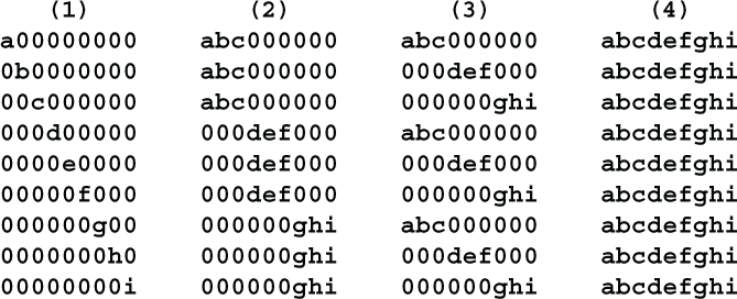
Now let’s analyze the SFlip cipher using the saturation index. After the first-round substitution, each bit of the ciphertext depends 1/3 on each of the 3 corresponding plaintext bits. The saturation matrix will look like (5). After the first-round flip, the saturation matrix will look like (6).
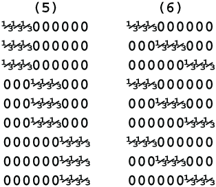
The second-round substitution makes each bit of the output dependent on all 9 bits of the first-round plaintext. The saturation coefficient is 1/3+(1/3)/2+(1/3)/4 = 1/3+1/6+1/12 = 7/12, about .583. Every element in the saturation matrix will have this value, so the saturation index will be 7/12. The target value for the saturation index is 1, although you could set it higher if you wanted greater certainty. Here is what the saturation index will be after several rounds.
So 3 rounds are sufficient for the 3×3 cipher, but 5 rounds are necessary for the 8×8 cipher.
Let’s now turn to some of the other situations where an output unit depends on one or more input units.
When an S-box has both plaintext and key inputs, say p plaintext units and k key units, the dependency for each of its output units will be 1/(p+k). For example, if the inputs are 6 key bits and 4 plaintext bits, the dependency will be 1/10 for each output bit. If the inputs to the S-box are themselves dependent on earlier inputs, then either the S1 or the S2 calculation should be used, as appropriate, to compute the saturation index.
Similarly, if two or more units are combined using exclusive-OR or some other combining function, the dependency is 1/n for n total inputs. The calculation of the saturation index is the same as for an S-box with the same inputs.
When a key of k bits is used for a transposition, each output unit of the transposition has a dependency of 1/k on each of the key bits, and a dependency of 1 on the plaintext input. Suppose that a plaintext character p is moved from position a to position b by the transposition. The saturation vector for p after the transposition will be the same as the saturation vector for p before the transposition, except in those columns corresponding to the bits of the transposition key. In those columns the saturation coefficient will be determined by either the S1 or S2 calculation.
Here is an example. Suppose that t is one of the bits of the transposition key. If p had no dependency on t before the transposition, that is, there was a 0 in column t of its saturation vector, then after the transposition the value in column t will be 1/k. On the other hand, if p were already dependent on the key bit t, then the saturation coefficient would be determined by the S2 calculation. If the coefficient in column t were x, then after the transposition the saturation coefficient in column t would be x+1/2k if x ≥ 1/k, or 1/k+x/2 if x < 1/k.
When a key of k bits has been used to mix the alphabet or tableau for a substitution step, the mixed alphabet or tableau has a dependency of 1/k on each bit of that key. Each time a character is substituted using that alphabet, the output character gets an additional dependency of 1/k on each bit of the key. This is combined with the dependencies of the input character (and substitution key, if any) using either the S1 or S2 calculation to get the saturation coefficient for the output character.
Summary
A block cipher will be unbreakable in practice if it adheres to all of these rules:
-
It has a sufficiently large block size. The current standard is 16 characters or 128 bits.
-
It has a sufficiently large key. The current standard is 128 to 256 bits. The key must be at least as large as the block, and preferably larger.
-
Either it uses fixed S-boxes that are strongly non-linear, or it uses variable substitution tables that are well-mixed using a large key.
As always, be conservative. Build yourself a safe margin of error. Make the key longer and use more rounds than required because computers get faster and new attacks get discovered continually. In particular, you could set your target for the saturation index higher than 1, perhaps 2, 3 or even 5.