CHAPTER 4

Accounting for Body Dynamics: The Jogger's Problem

Let me first explain to you how the motions of different kinds of matter depend on a property called inertia.

— Sir William Thomson (Lord Kelvin), The Tides

4.1 PROBLEM STATEMENT

As discussed before, motion planning algorithms usually adhere to one of the two paradigms that differ primarily by their assumptions about input information: motion planning with complete information (Piano Mover's problem) and motion planning with incomplete information (sensor-based motion planning, SIM paradigm, see Chapter 1). Strategies that come out of the two paradigms can be also classified into two groups: kinematic approaches, which consider only kinematic and geometric issues, and dynamic approaches, which take into account the system dynamics. This classification is independent from the classification into the two paradigms. In Chapter 3 we studied kinematic sensor-based motion planning algorithms. In this chapter we will study dynamic sensor-based motion planning algorithms.

What is so dynamic about dynamic approaches? In strategies that we considered in Chapter 3, it was implicitly assumed that whatever direction of motion is good for the robot's next step from the standpoint of its goal, the robot will be able to accomplish it. If this is true, in the terminology of control theory such a system is called a holonomic system [78]. In a holonomic system the number of control variables available is no less that the problem dimensionality. The system will also work as intended in situations where the above condition is not satisfied, but for some reason the robot dynamics can be ignored. For example, a very slowly moving robot can turn on a dime and hence can execute any sharp turn if prescribed by its motion planning software.

Most of existing approaches to motion planning (including those within the Piano Mover's model) assume, first, that the system is holonomic and, second, that it will behave as a holonomic system. Consequently, they deal solely with the system kinematics and ignore its dynamic properties. One reason for this state of affairs is that the methods of motion planning tend to rely on tools from geometry and topology, which are not easily connected to the tools common to control theory. Although system dynamics and sensor-based motion control are clearly tightly coupled in many, if not most, real-world systems, little attention has been paid to this connection in the literature.

The robot is a body; it has a mass and dimensions. Once it starts moving, it acquires velocity and acceleration. Its dynamics may now prevent it from making sharp, and sometimes even relatively shallow, turns prescribed by the planning algorithm. A sharp turn reasonable from the standpoint of reaching the target position may not be physically realizable because of the robot's inertia. In control theory terminology, this is a nonholonomic system [78]. A classical example of a nonholonomic control problem is the car parallel parking task: Because the driver does not have enough control means to execute the parking in one simple translational motion, he has to wiggle the car back and force to bring it to the desired position.

Given the insufficient information about the surroundings, which is central to the sensor-based motion planning paradigm, the lack of control means to execute any desired motion translates into a safety issue: One needs a guarantee of a stopping path at any time, in case a sudden obstacle makes it impossible to continue on the intended path.

Theoretically, there is a simple way out: We can make the robot stop every time it intends to turn, let it turn, and resume the motion as needed. Not many applications will like such a stop-and-go motion pattern. For a realistic control we want the robot to make turns on the move, and not stop unless “absolutely necessary,” whatever this means. That is, in addition to the usual problem of “where to go” and how to guarantee the algorithm convergence in view of incomplete information, the robot's mass and velocity bring about another component of motion planning, body dynamics. Furthermore, we will see that it will be important to incorporate the constraints of robot dynamics into the very motion planning algorithm, together with the constraints dictated by collision avoidance and algorithm convergence requirements.

We call the problem thus formulated the Jogger's Problem, because it is not unlike the task a human jogger faces in an urban setting when going for a morning run. Taking a run involves continuous on-line control and decision-making. Many decisions will be made during the run; in fact, many decisions are made within each second of the run. The decision-making apparatus requires a smooth collaboration of a few mechanisms. First, a global planning mechanism will work on ensuring arrival at the target location in spite of all deviations and detours that the environment may require. Unless a “grand plan” is followed, arrival at the target location—what we like to call convergence—may not be guaranteed.

Second, since an instantaneous stop is impossible due to the jogger's inertia, in order to maintain a reasonable speed the jogger needs at any moment an “insurance” option of a safe stopping path. This mechanism will relate the jogger's mass and speed to the visible field of view. It is better to slow down at the corner—who knows what is behind the corner?

Third, when the jogger starts turning the street corner and suddenly sees a pile of sand right on the path that he contemplated (it was not there last time), some quick local planning must occur to take care of collision avoidance. The jogger's speed may temporarily decrease and the path will smoothly divert from the object. The jogger will likely want to locally optimize this path segment, in order to come back to his preplanned path quicker or along a shorter path. Other options not being feasible, the jogger may choose to “brake” to a halt and start a detour path.

As we see, the jogger's speed, mass, and quality of vision, as well as the speed of reaction to sudden changes—which represents the quality of his control system—are all tied together in a certain relationship, affecting the real-time decision-making process. The process will go on nonstop, all the time; the jogger cannot afford to take his eyes off the route for more than a fraction of a second. Sensing, local planning, global planning, and actual movement are in this process taking place simultaneously and continuously. Locally, unless the right relationship is maintained between the velocity when noticing an object, the distance to it, and the jogger's mass, collision may occur. A bigger mass may dictate better (farther) sensing to maintain the same velocity. Myopic vision may require reducing the speed.

Another interesting detail is that in the motion planning strategies considered in Chapter 3, each step of the path could be decided independently from other steps. The control scheme that takes into account robot dynamics cannot afford such luxury anymore. Often a decision will likely affect more than calculation of the current step. Consider this: Instead of turning on the dime as in our prior algorithms, the robot will be likely moving along relatively smooth curves. How do we know that the smooth path curve dictated by robot dynamics at the current step will not be in conflict with collision considerations at the next step? Perhaps at the current step we need to think of the next step as well. Or perhaps we need to think of more than one step ahead. Worse yet, what if a part of that path curve cannot be checked because it is bending around the corner of a nearby obstacle and hence is invisible?

These questions suggest that in a planning/control system with included dynamics a path step cannot be planned separately from at least a few steps that will follow it. The robot must make sure that the step it now contemplates will not result in some future steps where the collision is inevitable. How many steps look-ahead is enough? This is one thing that we need to figure out.

Below we will study the said effects, with the same objective as before—to design provably correct sensor-based motion planning algorithms. As before, the presence of uncertainty implies that no global optimality of the path is feasible. Notice, however, that given the need to plan for a few steps ahead, we can attempt local optimization. While improving the overall path, sometimes dramatically, in general a path segment that is optimal within the robot's field of vision says nothing about the path global optimality.

By the way, which optimization criterion is to be used? We will consider two criteria. The salient feature of one criterion is that, while maintaining the maximum velocity allowed by its dynamics, the robot will attempt to maximize its instantaneous turning angle toward the required direction of motion. This will allow it to finish every turning maneuver in minimum time. In a path with many turns, this should save a good deal of time. In the second strategy (which also assumes the maximum velocity compatible with collision avoidance), the robot will attempt a time-optimal arrival at its (constantly shifting) intermediate target. Intermediate targets will typically be on the boundary of the robot's field of vision.

Similar to the model used in Chapter 3, our mobile robot operates in two-dimensional physical space filled with a locally finite number of unknown stationary obstacles of arbitrary shapes. Planning is done in small steps (say, 30 or 50 times per second, which is typical for real-world robotics), resulting in continuous motion. The robot is equipped with sensors, such as vision or range finders, which allow it to detect and measure distances to surrounding objects within its sensing range. Robot vision works within some limited or unlimited radius of vision, which allows some steps look-ahead (say, 20 or 30 or more). Unless obstacles occlude one another, the robot will see them and use this information to plan appropriate actions. Occlusions effectively limit a robot's input information and call for more careful planning.

Control of body dynamics fits very well into the feedback nature of the SIM (Sensing-Intelligence-Motion) paradigm. To be sure, such control can in principle be incorporated in the Piano Mover's paradigm as well. One way to do this is, for example, to divide the motion planning process into two stages: First, a path is produced that satisfies the geometric constraints, and then this path is modified to fit the dynamic constraints [79], possibly in a time-optimal fashion [80–82].

Among the first attempts to explicitly incorporate body dynamics into robot motion planning were those by O'Dunlaing [83] for the one-dimensional case and by Canny et al. [84] in their kinodynamic planning approach for the two-dimensional case. In the latter work the proposed algorithm was shown to run in exponential time and to require space that is polynomial in the input. While the approach operates in the context of the Piano Mover's paradigm, it is somewhat akin to the approach considered in this chapter, in that the control strategy adheres to the L_∞-norm; that is, the velocity and acceleration components are assumed bounded with respect to a fixed (absolute) reference system. This allows one to decouple the equations of robot motion and treat the two-dimensional problem as two one-dimensional problems.¹

Within the Piano Mover's paradigm, a number of kinematic holonomic strategies make use of the artificial potential field. They usually require complete information and analytical presentation of obstacles; the robot's motion is affected by (a) the “repulsive forces” created by a potential field associated with obstacles and (b) “attractive forces” associated with the goal position [85]. A typical convergence issue here is how to avoid possible local minima in the potential field. Modifications that attempt to solve this problem include the use of repulsive fields with elliptic isocontours [86], introduction of special global fields [87], and generation of a numerical field [88]. The vortex field method [89] allows one to avoid undesirable attraction points, while using only local information; the repulsive actions are replaced by the velocity flows tangent to the isocontours, so that the robot is forced to move around obstacles. An approach called active reflex control [90] attempts to combine the potential field method with handling the robot dynamics; the emphasis is on local collision avoidance and on filtering out infeasible control commands generated by the motion planner.

Among the approaches that deal with incomplete information, a good number of holonomic techniques originate in maze-search strategies (see the previous chapters). When applicable, they are usually fast, can be used in real time, and guarantee convergence; obstacles in the scene may be of arbitrary shape.

There is also a group of nonholonomic motion planning approaches that ignore the system dynamics. These also require analytical representation of obstacles and assume complete [91–93] or partial input information [94]. The schemes are essentially open-loop, do not guarantee convergence, and attempt to solve the planning problem by taking into account the effect of nonholonomic constraints on obstacle avoidance. In Refs. 91 and 92 a two-stage scheme is considered: First, a holonomic planner generates a complete collision-free path, and then this path is modified to account for nonholonomic constraints. In Ref. 93 the problem is reduced to searching a graph representing the discretized configuration space. In Ref. 94, planning is done incrementally, with partial information: First, a desirable path is defined and then a control is found that minimizes the error in a least-squares sense.

To design a provably correct dynamic algorithm for sensor-based motion planning, we need a single control mechanism: Separating it into stages is likely to destroy convergence. Convergence has two faces: Globally, we have to guarantee finding a path to the target if one exists. Locally, we need an assurance of collision avoidance in view of the robot inertia. The former can be borrowed from kinematic algorithms; the latter requires an explicit consideration of dynamics.

Notice an interesting detail: In spite of sufficient knowledge about the piece of the scene that is currently within the robot's sensing range, even in this area it would make little sense at a given step to address the planning task as one with complete information, as well as to try to compute the whole subpath within the sensing range. Why not? Computing this subpath would require solving a rather difficult optimal motion control problem—a computationally expensive task. On the other hand, this would be largely computational waste, because only the first step of this subpath would be executed: As new sensing data appears at the next step, in general a path adjustment would be required. We will therefore attempt to plan only as many steps that immediately follow the current one as is needed to guarantee nonstop collision-free motion.

The general approach will be as follows: At its current position C_i, the robot will identify a visible intermediate target point, T_i, that is guaranteed to lie on a convergent path and is far enough from the robot—normally at the boundary of the sensing range. If the direction toward T_i differs from the current velocity vector V_i, moving toward T_i may require a turn, which may or may not be possible due to system dynamics.

In the first strategy that we will consider, if the angle between V_i and the direction toward T_i is larger than the maximum turn the robot can make in one step, the robot will attempt a fast smooth maneuver by turning at the maximum rate until the directions align; hence the name Maximum Turn Strategy. Once a step is executed, new sensing data appear, a new point T_i+1 is sought, and the process repeats. That is, the actual path and the path that contains points T_i will likely be different paths: With the new sensory data at the next step, the robot may or may not be passing through point T_i.

In the second strategy, at each step, a canonical solution is found which, if no obstacles are present, would bring the robot from its current position C_i to the intermediate target T_i with zero velocity and in minimum time. Hence the name Minimum Time Strategy. (The minimum time refers of course to the current local piece of scene.) If the canonical path crosses an obstacle and is thus not feasible, a near-canonical solution path is found which is collision-free and satisfies the control constraints. We will see that in this latter case only a small number of options needs be considered, at least one of which is guaranteed to be collision-free.

The fact that no information is available beyond the sensing range dictates caution. To guarantee safety, the whole stopping path must not only lie inside the sensing range, it must also lie in its visible part. No parts of the stopping path can be occluded by obstacles. Moreover, since the intermediate target T_i is chosen as the farthest point based on the information currently available, the robot needs a guarantee of stopping at T_i, even if it does not intend to do so. Otherwise, what if an obstacle lurks right beyond the vision range? That is, each step is to be planned as the first step of a trajectory which, given the current position, velocity, and control constraints, would bring the robot to a halt at T. Within one step, the time to acquire sensory data and to calculate necessary controls must fit into the step cycle.

4.2 MAXIMUM TURN STRATEGY

4.2.1 The Model

The robot is a point mass, of mass m. It operates in the plane; the scene may include a locally finite number of static obstacles. Each obstacle is bounded by a simple closed curve of arbitrary shape and of finite length, such that a straight line will cross it in only a finite number of points. Obstacles do not touch each other; if they do, they are considered one obstacle. The total number of obstacles in the scene need not be finite.

The robot's sensors provide it with information about its surroundings within the sensing range (radius of vision), a disc of radius r_υ centered at its current location C_i. The sensor can assess the distance to the nearest obstacle in any direction within the sensing range. The robot input information at moment t_i includes its current velocity vector V_i, coordinates of point C_i and of the target point T, and possibly few other points of interest that will be discussed later.

The task is to move, collision-free, from point S (start) to point T (target) (see Figure 4.1). The robot's control means include two components (p, q) of the acceleration vector , where m is the robot mass and f is the force applied. Though the units of (p, q) are those of acceleration, by normalizing to m = 1 we can refer to p and q as control forces, each within its fixed range |p| ≤ p_max, |q| ≤ q_max. Force p controls forward (or backward when braking) motion; its positive direction coincides with the velocity vector V. Force q is perpendicular to p, forming a right pair of vectors, and is equivalent to the steering control (rotation of vector V) (Figure 4.2). Constraints on p and q imply a constraint on the path curvature. The point mass assumption implies that the robot's rotation with respect to its “center of mass” has no effect on the system dynamics. There are no external forces acting on the robot except p and q. There is no friction; for example, values p = q = 0 and V ≠ 0 will result in a straight-line constant velocity motion.²

Robot motion is controlled in steps i, i = 0, 1, 2,…. Each step takes time δt = t_i+1 − t_i = const. The step's length depends on the robot's velocity within the step. Steps i and i + 1 start at times t_i and t_i+1, respectively; C₀ = S. While moving toward location C_i+1, the robot computes necessary controls for step i + 1 using the current sensory data, and it executes them at C_i+1. The finite time necessary within one step for acquiring sensory data, calculating the controls, and executing the step must fit into the step cycle (more details on this can be found in Ref. 96). We define two coordinate systems (follow Figure 4.2):

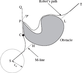
Figure 4.1 An example of a conflict between the performance of a kinematic algorithm (e.g., VisBug-21, the solid line path) and the effects of dynamics (the dotted piece of trajectory at P).

Figure 4.2 The path coordinate frame (t, n) is used in the analysis of dynamic effects of robot motion. The world frame (x, y), with its origin at the start point S, is used in the obstacle detection and path planning analysis.

• The world coordinate frame, (x, y), fixed at point S.
• The path coordinate frame, (t, n), which describes the motion of point mass at any moment τ ∈ [t_i, t_i+1) within step i. The frame's origin is attached to the robot; axis t is aligned with the current velocity vector V; axis n is normal to t; that is, when V = 0, the frame is undefined. One may note that together with axis b = t × n, the triple (t, n, b) forms the known Frenet trihedron, with the plane of t and n being the osculating plane [97].

4.2.2 Sketching the Approach

Some terms and definitions here are the same as in Chapter 3; material in Section 3.1 can be used for more rigorous definitions. Define M-line (Main line) as the straight-line segment (S, T) (Figure 4.1). The M-line is the robot's desired path. When, while moving along the M-line, the robot senses an obstacle crossing the M-line, the crossing point on the obstacle boundary is called a hit point, H. The corresponding M-line point “on the other side” of the obstacle is a leave point, L.

The planning procedure is to be executed at each step of the robot's path. Any provable maze-searching algorithm can be used for the kinematic part of the algorithm that we are about to build, as long as it allows distant sensing. For specificity only, we use here the VisBug algorithm (see Section 3.6; either VisBug-21 or VisBug-22 will do). VisBug algorithms alternate between these two operations (see Figure 4.1):

1. Walk from point S toward point T along the M-line until, at some point C, you detect an obstacle crossing the M-line, say at point H.
2. Using sensing data, define the farthest visible intermediate target T_i on the obstacle boundary and on a convergent path; make a step toward T_i; iterate Step 2 until you detect the M-line; go to Step 1.

To this process we add a control procedure for handling dynamics. It is clear already that from time to time dynamics will prevent the robot from carefully following an obstacle boundary. For example, in Figure 4.1, while trying to pass the obstacle from the left, under a VisBug procedure the robot would make a sharp turn at point P. Such motion is not possible in a system with dynamics.

At times the current intermediate target T_i may go out of the robot's sight, because of the robot inertia or because of occluding obstacles. In such cases the robot will be designating temporary intermediate targets and use them until it can spot the point T_i again. The final algorithm will also include mechanisms for checking the target reachability and for local path optimization.

4.2.3 Velocity Constraints. Minimum Time Braking

By substituting p_max for p and r_υ for d into (4.1), one obtains the maximum velocity, V_max. Since the maximum distance for which sensing information is available is r_υ, the sensing range boundary, an emergency stop should be planned for that distance. We will show that moving with the maximum speed—certainly a desired feature—actually guarantees a minimum-time arrival at the sensing range boundary. The suggested braking procedure, developed fully in Section 4.2.4, makes use of an optimization scheme that is sketched briefly in Section 4.2.4.

4.2.4 Optimal Straight-Line Motion

We now sketch the optimization scheme that will later be used in the development of the braking procedure. Consider a dynamic system, a moving body whose behavior is described by a second-order differential equation , where || p(t) || ≤ p_max and p(t) is a scalar control function. Assume that the system moves along a straight line. By introducing state variables x and V, the system equations can be rewritten as and . It is convenient to analyze the system behavior in the phase space (V, x).

The goal of control is to move the system from its initial position (x(t₀), V(t₀)) to its final position (x(t_f), V(t_f)). For convenience, choose x(t_f) = 0. We are interested in an optimal control strategy that would execute the motion in minimum time t_f, arriving at x(t_f) with zero velocity, V(t_f) = 0. This optimal solution can be obtained in closed form; it depends upon the above/below relation of the initial position with respect to two parabolas that define the switch curves in the phase plane (V, x):

This simple result in optimal control (see, e.g., Ref. 98) is summarized in the control law that follows, and it is used in the next section in the development of the braking procedure for emergency stopping. The procedure will guarantee robot safety while allowing it to cruise with the maximum velocity (see Figure 4.4):

Figure 4.4 Depending on whether the initial position (V₀, x₀) in the phase space (V, x) is above or below the switch curves, there are two cases to consider. The optimal solution corresponds to moving first from point (V₀, x₀) to the switching point (V_s, x_s) and then along the switch line to the origin.

and then, with control , toward the origin, along parabola II,

The optimal time t_b of braking is a function of the initial velocity V₀, radius of vision r_υ, and the control limit p_max,

Function t_b(V₀) has a minimum at which is exactly the upper bound on the velocity given by (4.1); it is decreasing on the interval V₀ ∈ [0, V_max] and increasing when V₀ > V_max (see Figure 4.5b). For the interval V₀ ∈ [0, V_max], which is of interest to us, the above analysis leads to a somewhat counterintuitive conclusion:

Notice that this result (see also Figure 4.5) leaves a comfortable margin of safety: Even if at the moment when the robot sees an obstacle on its way it moves with the maximum velocity, it can still stop safely before it reaches the obstacle. If the robot's velocity is below the maximum, it has more control options for braking, including even one of speeding up before actual braking. Assume, for example, that we want the robot to stop in minimum time at the sensing range boundary (the origin in Figure 4.5a); consider two initial positions: and . Then, according to Proposition 1, in case (i) this time is bigger than in case (ii). Note that because of the discrete control it is the permitted maximum velocity, V_{p max}, that is to be substituted into (4.4) to obtain the minimum time. (More details on the braking procedure can be found in Ref. 99).

4.2.5 Dynamics and Collision Avoidance

The analysis in this section consists of two parts. First we incorporate the control constraints into the model of our mobile robot and develop a transformation from the moving path coordinate frame to the world frame (see Section 4.2.1). Then the Maximum Turn Strategy is produced, an incremental decision-making mechanism that determines forces p and q at each step.

The angle θ between vector V and x axis of the world frame is found as

To find the transformation from path frame to the world frame (x, y), present the velocity in the path frame as V = Vt. Angle θ is defined as the angle between t and the positive direction of x axis. Given that control forces p and q act along the t and n directions, respectively, the equations of motion with respect to the path frame are

Since the control forces are constant over time interval [t_i, t_i+1), within this interval the solution for V(t) and θ(t) becomes

where θ₀ and V₀ are constants of integration and are equal to the values of θ(t_i) and V(t_i), respectively. By parameterizing the path by the value and direction of the velocity vector, the path can be mapped onto the world frame using the vector integral equation

Here r(t) = (x(t), y(t)) and V = (V · cos(θ), V · sin(θ)) are the projections of vector V onto the world frame (x, y). After integrating Eq. (4.6), we obtain a set of solutions in the form

where terms A and B are

Equations (4.7) are directly defined by the control variables p and q; V(t) and θ(t) therein are given by Eq. (4.5).

In general, Eqs. (4.7) describe a spiral curve. Note two special cases: When p ≠ 0, q = 0, Eqs. (4.7) describe a straight-line motion along the vector of velocity; when p = 0 and q ≠ 0, Eqs. (4.7) produce a circle of radius centered at the point (A, B).

where q = +q_max if the intermediate target T_i lies in the left semiplane, and q = −q_max if T_i lies in the right semiplane with respect to the vector of velocity. That is, force p is chosen so as to keep the maximum velocity allowed by the surrounding obstacles. To this end, a discrete set of values p is tried until a step that guarantees a collision-free stopping path is found. At a minimum, the set should include values −p_max, 0, and +p_max. The greater the number of values that are tried, the closer the resulting velocity is to the maximum sought. Force q is chosen on the boundary, to produce a maximum turn in the appropriate direction. On the other hand, if because of obstacles no adequate controls in the range (4.8) can be chosen, this means that maximum braking should be applied. Then the controls are chosen from the set

where q is found from a discrete set similar to p in (4.8). Note that sets (4.8) and (4.9) always include at least one safe solution: By the algorithm design, the straight-line motion with maximum braking, (p, q) = (−p_max, 0), is always collision-free (for more detail, see Ref. 96).

4.2.6 The Algorithm

The resulting algorithm consists of three procedures:

• Main Body. This defines the motion within the time interval [t_i, t_i+1) toward the intermediate target T_i.
• Define Next Step. This chooses the forces p and q.
• Find Lost Target. This handles the case when the intermediate target goes out of the robot's sight.

Also used in the algorithm is a procedure called Compute T_i, from the VisBug algorithms (Section 3.6), which computes the next intermediate target T_i+1 and includes a test for target reachability. Vector V_i, is the current vector of velocity, and T is the robot's target location. The term “safe motion” below refers to the mechanism for determining the next robot's position C_i+1 such as to guarantee a stopping path (Section 4.2.2).

• M1: Move in the direction specified by Define Next Step, while executing Compute T_i. If T_i is visible, do the following: If C_i = T, the procedure stops; else if T is unreachable, the procedure stops; else if C_i = T_i, go to M2. Otherwise, use Find Lost Target to make T_i visible. Iterate M1.
• M2: Make a step along vector V_i while executing Compute T_i: If C_i = T, the procedure stops; else if the target is unreachable, the procedure stops; else if C_i ≠ T_i, go to M1.

• D1: If vector V_i coincides with the direction toward T_i, do the following: If T_i = T, make a step toward T; else make a step toward T_i.
• D2: If vector V_i does not coincide with the direction toward T_i, do the following: If the directions of V_i+1 and (C_i, T_i) can be aligned within one step, choose this step. Else go to D3.
• D3: If a step with the maximum turn toward T_i and with maximum velocity is safe, choose it. Else go to D4.
• D4: If a step with the maximum turn toward T_i and some braking is possible, choose it. Else, choose a step along V_i, with maximum braking, p = −p_max, q = 0.

• F1: If segment (C_i, T_i) is visible, define on it a temporary intermediate target and move toward it while looking for T_i. If the current position is at T, exit; else if C_i lies in the segment (C_i, T_i), exit. Else go to F2.
• F2: If segment (C_i, T_i) is invisible, initiate a stopping path and move back to C_i; exit.

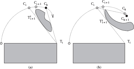
Figure 4.6 Because of its inertia, immediately after its position C_i the robot temporarily “loses” the target intermediate T_i. (a) The robot keeps moving around the obstacle until it spots T_i, and then it continues toward T_i. (b) When because of an obstacle the whole segment (C_i, T_i) becomes invisible at point C_k+1, the robot stops, returns back to C_i, and then moves toward T_i along the line (C_i, T_i).

By design, the stopping path is a straight-line segment. Choosing the next step so as to guarantee existence of a stopping path implies two requirements: There should be at least one safe direction of motion and the value of velocity that would allow stopping within the visible area. The latter is ensured by the choice of system parameters [see Eq. (4.1) and the safety conditions, Section 4.2.2]. As to the existence of safe directions, proceed by induction: We need to show that if a safe direction exists at the start point and at an arbitrary step i, then there is a safe direction at the step (i + 1).

Since at the start point S the velocity is zero, V_s = 0, then any direction of motion at S will be a safe direction; this gives the basis of induction. The induction proceeds as follows. Under the algorithm, a candidate step is accepted for execution if only its direction guarantees a safe stop for the robot if needed. Namely, at point C_i, step i is executed only if the resulting vector V_i+1 at C_i+1 will point in a safe direction. Therefore, at step (i + 1), at the least this very direction presents a safe stopping path.

To see this, note that by design of the VisBug algorithm (see Section 3.6.3), each intermediate target T_i lies on a convergent path and is visible at the moment when it is generated.

That is, the only way the robot can get lost is if at the following step(s) point T_i becomes invisible due to the robot's inertia or an obstacle occlusion: This would make it impossible to generate the next intermediate target, T_i+1, as required by VisBug. However, if point T_i does become invisible, the procedure Find Lost Target is invoked, a set of temporary intermediate targets are defined, each with a guaranteed stopping path, and more steps are executed until point T_i becomes visible again (see Figure 4.6). The set is finite because of finite distances between every pair of points in it and because the set must lie within the sensing range of radius r_υ. Therefore, the robot always moves toward a point which lies on a path that is convergent to the target T.

4.2.7 Examples

Examples shown in Figures 4.7a to 4.7d demonstrate performance of the Maximum Turn Strategy in a computer simulated environment. Generated paths are shown by thicker lines. For comparison, also shown by thin lines are paths produced under the same conditions by the VisBug algorithm. Polygonal shapes are chosen for obstacles in the examples only for the convenience of generating the scene; the algorithms are oblivious to the obstacle shapes.

To understand the examples, consider a simplified version of the relationship that appears in Section 4.2.3, . In the simulations, the robot's mass m and control force f_max are kept constant; for example, an increase in sensing radius r_υ would “raise” the velocity V_max. Radius r_υ is the same in Figures 4.7a and 4.7b. In the more complex scene (b), because of three additional obstacles (three small squares) the robot's path cannot curve as freely as in scene (a). Consequently, the robot moves more “cautiously,” that is, slower; the path becomes tighter and closer to the obstacles, allowing the robot to squeeze between obstacles. Accordingly, the time to complete the path is 221 units (steps) in (a) and 232 units in (b), whereas the path in (a) is longer than that in (b).

Figure 4.7 In each of the four examples shown, one path (indicated by the thin line) is produced by the VisBug algorithm, and the other path (a thicker line) is produced by the Maximum Turn Strategy, which takes into account the robot dynamics. The circle at point S indicates the radius of vision r_υ.

Figures 4.7c and 4.7d refer to a more complex environment. The difference between these two situations is that in (d) the radius of vision r_υ is 1.5 times larger than that in (c). Note that in (d) the path produced by the Maximum Turn Strategy is noticeably shorter than the path generated by the VisBug algorithm. This has happened by sheer chance: Unable to make a sharp turn (because of its inertia) at the last piece of its path, the robot “jumped out” around the corner and hence happened to be close enough to T to see it, and this eliminated a need for more obstacle following.

Note the stops along the path generated by the Maximum Turn Strategy; they are indicated by sharp turns. These might have been caused by various reasons: For example, in Figure 4.7a the robot stopped because its small sensing radius r_υ was insufficient to see the obstacle far enough to initiate a smooth turn. In Figure 4.7d, the stop at point P was probably caused by the robot's temporarily losing its current intermediate target.

4.3 MINIMUM TIME STRATEGY

We will now consider the second strategy for solving the Jogger's Problem. The same model of the robot, its environment, and its control means will be used as in the Maximum Turn Strategy (see Section 4.2.1).

The general strategy will be as follows: At the given step i, the kinematic motion planning procedure chosen—we will use again VisBug algorithms— identifies an intermediate target point, T_i, which is the farthest visible point on a convergent path. Normally, though not always, T_i is defined at the boundary of the sensing range r_υ. Then a single step that lies on a time-optimal trajectory to T_i is calculated and executed; the robot moves from its current position C_i to the next position C_i+1, and the process repeats.

Similar to the Maximum Turn Strategy, the fact that no information is available beyond the robot's sensing range dictates a number of requirements. There must be an emergency stopping path, and it must lie inside the current sensing area. Since parts of the sensing range may be occupied or occluded by obstacles, the stopping path must lie in its visible part. Next, the robot needs a guarantee of stopping at the intermediate target T_i, even if it does not intend to do so. That is, each step is to be planned as the first step of a trajectory which, given the robot's current position, velocity, and control constraints, would bring it to a halt at T_i (though, again, this will be happening only rarely).

The step-planning task is formulated as an optimization problem. It is the optimization criterion and procedure that will make this algorithm quite different from the Maximum Turn Strategy. At each step, a canonical solution is found which, if no obstacles are present, would bring the robot from its current position C_i to its current intermediate target T_i with zero velocity and in minimum time. If the canonical path happens to be infeasible because it crosses an obstacle, a collision-free near-canonical solution path is found. We will show that in this case only a small number of path options need be considered, at least one of which is guaranteed to be collision-free.

By making use of the L_∞-norm within the duration of a single step, we decouple the two-dimensional problem into two one-dimensional control problems and reduce the task to the bang-bang control strategy. This results in an extremely fast procedure for finding the time-optimal subpath within the sensing range. The procedure is easily implementable in real time. Since only the first step of this subpath is actually executed—the following step will be calculated when new sensor information appears after this (first) step is executed—this decreases the error due to the control decoupling. Then the process repeats. One special case will have to be analyzed and incorporated into the procedure—the case when the intermediate target goes out of the robot's sight either because of the robot inertia or because of occluding obstacles.

4.3.1 The Model

To a large extent the model that we will use in this section is similar to the model used by the Maximum Turn Strategy above. There are also some differences. For convenience we hence give a complete model description here.

As before, the scene is two-dimensional physical space it may include a finite set of locally finite static obstacles . Each obstacle is a simple closed curve of arbitrary shape and of finite length, such that a straight line will cross it in only a finite number of points. Obstacles do not touch each other; if they do, they are considered one obstacle.

The robot is a point mass, of mass m. Its vision sensor allows it to detect any obstacles and the distance to them within its sensing range (radius of vision)—a disk D(C_i, r_υ) of radius r_υ centered at its current location C_i. At moment t_i, the robot's input information includes its current velocity vector V_i and coordinates of C_i and of target location T.

The robot's means to control its motion are two components of the acceleration vector u = f/m = (p, q), where m is the robot mass and f the force applied. Controls u come from a set u(·) ∈ U of measurable, piecewise continuous bounded functions in ℜ², U = {u(·) = (p(·), q(·))/p ∈ [−p_max, p_max], q ∈ [−q_max, q_max]}. By taking mass m = 1, we can refer to components p and q as control forces, each within a fixed range |p| ≤ p_max, |q| ≤ q_max; p_max, q_max > 0. Force p controls the forward (or backward when braking) motion; its positive direction coincides with the robot's velocity vector V. Force q, the steering control, is perpendicular to p, forming a right pair of vectors (Figure 4.8). There is no friction: For example, given velocity V, the control values p = q = 0 will result in a constant-velocity straight-line motion along the vector V.

Without loss of generality, assume that no external forces except p and q act on the system. Note that with this assumption our model and approach can still handle other external forces and constraints using, for example, the technique suggested in Ref. 95, whereby various dynamic constraints such as curvature, engine force, sliding, and velocity appear in the inequality describing the limitations on the components of acceleration. The set of such inequalities defines a convex region of the space. In our case the control forces act within the intersection of the box [−p_max, p_max] × [−q_max, q_max], with the half-planes defined by those inequalities.

The task is to move in from point S (start) to point T (target) (see Figure 4.1). The control of robot motion is done in steps i, i = 0, 1, 2,… Each step i takes time δt = t_i+1 − t_i = const; the path length within time interval δt depends on the robot velocity V_i. Steps i and i + 1 start at times t_t and t_i+1, respectively; C₀ = S. Control forces u(·) = (p, q) ∈ U are constant within the step.

We define three coordinate systems (follow Figure 4.8):

• The world frame, (x, y), is fixed at point S.
• The primary path frame, (t, n), is a moving (inertial) coordinate frame. Its origin is attached to the robot; axis t is aligned with the current velocity vector V, axis n is normal to t. Together with axis b, which is a cross product b = t × n, the triple (t, n, b) forms the Frenet trihedron, with the plane of t and n forming the osculating plane [97].
• The secondary path frame, (ξ_i, η_i), is a coordinate frame that is fixed during the time interval of step i. The frame's origin is at the intermediate target T_i; axis ξ_i is aligned with the velocity vector V_i at time t_i, and axis η_i is normal to ξ_i.

For convenience we combine the requirements and constraints that affect the control strategy into a set, called Ω. A solution (a path, a step, or a set of control values) is said to be Ω-acceptable if, given the current position C_i and velocity V_i,

(i) it satisfies the constraints |p| ≤ p_max, |q| ≤ q_max on the control forces,

(ii) it guarantees a stopping path,

(iii) it results in a collision-free motion.

4.3.2 Sketching the Approach

The algorithm that we will now present is executed at each step of the robot path. The procedure combines the convergence mechanism of a kinematic sensor-based motion planning algorithm with a control mechanism for handling dynamics, resulting in a single operation. As in the previous section, during the step time interval i the robot will maintain within its sensing range an intermediate target point T_i, usually on an obstacle boundary or on the desired path. At its current position C_i the robot will plan and execute its next step toward T_i. Then at C_i+1 it will analyze new sensory data and define a new intermediate target T_i+1, and so on. At times the current T_i may go out of the robot's sight because of its inertia or due to occluding obstacles. In such cases the robot will rely on temporary intermediate targets until it can locate point T_i again.

1. Walk from S toward T along the M-line until detect an obstacle crossing the M-line, say at point H. Go to Step 2.
2. Define a farthest visible intermediate target T_i on the obstacle boundary in the direction of motion; make a step toward T_i. Iterate Step 2 until detect M-line. Go to Step 1.

The actual algorithm will include additional mechanisms, such as a finite-time target reachability test and local path optimization. In the example shown in Figure 4.1, note that if the robot walked under a kinematic algorithm, at point P it would make a sharp turn (recall that the algorithm assumes holonomic motion). In our case, however, such motion is not possible because of the robot inertia, and so the actual motion beyond point P would be something closer to the dotted path.

where d is the distance from the robot to the stop point. That is, if the robot moves with the maximum velocity, the stop point of the stopping path must be no further than r_υ from the current position C. In practice, Eq. (4.10) can be interpreted in a number of ways. Note that the maximum velocity is proportional to the acceleration due to control, which is in turn directly proportional to the force applied and inversely proportional to the robot mass m. For example, if mass m is made larger and other parameters stay the same, the maximum velocity will decrease. Conversely, if the limits on (p, q) increase (say, due to more powerful motors), the maximum velocity will increase as well. Or, an increase in the radius r_υ (say, due to better sensors) will allow the robot to increase its maximum velocity, by the virtue of utilizing more information about the environment.

Consider the example in Figure 4.1. When approaching point P along its path, the robot will see it at distance r_υ and will designate it as its next intermediate target T_i. Along this path segment, point T_i happens to stay at P because no further point on the obstacle boundary will be visible until the robot arrives at P. Though there may be an obstacle right around the corner P, the robot needs not to slow down since at any point of this segment there is a possibility of a stopping path ending somewhere around point Q. That is, in order to proceed with maximum velocity, the availability of a stopping path has to be ascertained at every step i. Our stopping path will be a straight-line path along the corresponding vector V_i. If a candidate step cannot guarantee a stopping path, it is discarded.⁴

4.3.3 Dynamics and Collision Avoidance

Consider a time sequence σ_t = {t₀, t₁, t₂, …, } of the starting moments of steps. Step i takes place within the interval [t_i, t_i+1), (t_i+1 − t_i) = δt. At moment t_i the robot is at the position C_i, with the velocity vector V_i. Within this interval, based on the sensing data, intermediate target T_i (supplied by the kinematic planning algorithm), and vector V_i, the control system will calculate the values of control forces p and q. The forces are then applied to the robot, and the robot executes step i, finishing it at point C_i+1 at moment t_i+1, with the velocity vector V_i+1. Then the process repeats.

Analysis that leads to the procedure for handling dynamics consists of three parts. First, in the remainder of this section we incorporate the control constraints into the robot's model and develop transformations between the primary path frame and world frame and between the secondary path frame and world frame. Then in Section 4.3.4 we develop the canonical solution. Finally, in Section 4.3.5 we develop the near-canonical solution, for the case when the canonical solution would result in a collision. The resulting algorithm operates incrementally; forces p and q are computed at each step. The remainder of this section refers to the time interval [t_i, t_i+1) and its intermediate target T_i, and so index i is often dropped.

Denote (x, y) ∈ ℜ² the robot's position in the world frame, and denote θ the (slope) angle between the velocity vector and x axis of the world frame (Figure 4.8). The planning process involves computation of the controls u = (p, q), which for every step define the velocity vector and eventually the path, (x(t), y(t)), as a function of time. Taking mass m = 1, the equations of motion become

Figure 4.8 The coordinate frame (x, y) is the world frame, with its origin at S; (t, n) is the primary path frame, and (ξ_i, η_i) is the secondary path frame for the current robot position C_i.

The angle θ between vector V = (V_x, V_y) and x axis of the world frame is found as

The transformations between the world frame and secondary path frame, from (x, y) to (ξ, η) and from (ξ, η) to (x, y), are given by

and

where

Since p and q are constant over the time interval t ∈ [t_i, t_i+1), the solution for V(t) and θ(t) within the interval becomes

where θ₀ and V₀ are constants of integration and are equal to the values of θ(t_i) and V(t_i), respectively. By parameterizing the path by the value and direction of the velocity vector, the path can be mapped into the world frame (x, y) using the vector integral equation

Here r(t) = (x(t), y(t)), and t is a unit vector of direction V, with the projections t = (cos(θ), sin(,θ)) onto the world frame (x, y). After integrating Eq. (4.14), obtain the set of solutions

where terms A and B are

and V(t) and θ(t) are given by (4.13).

Equations (4.15) describe a spiral curve. Note two special cases: When p ≠ 0 and q = 0, Eqs. (4.15) describe a straight-line motion under the force along the vector of velocity; when p = 0 and q ≠ 0, the force acts perpendicular to the vector of velocity, and Eqs. (4.15) produce a circle of radius centered at the point (A, B).

4.3.4 Canonical Solution

Given the current position C_i = (x_i, y_i), the intermediate target T_i, and the velocity vector , the canonical solution presents a path that, assuming no obstacles, would bring the robot from C_i to T_i with zero velocity and in minimum time. The L_∞-norm assumption allows us to decouple the bounds on accelerations in ξ and η directions, and thus treat the two-dimensional problem as a set of two one-dimensional problems, one for control p and the other for control q. For details on obtaining such a solution and the proof of its sufficiency, refer to Ref. 99.

The optimization problem is formulated based on the Pontryagin's optimality principle [100], with respect to the secondary frame (ξ, η). We seek to optimize a criterion F, which signifies time. Assume that the trajectory being sought starts at time t = 0 and ends at time t = t_f (for “final”). Then, the problem at hand is

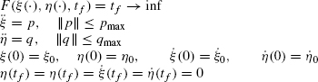
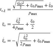
Analysis shows (see details in the Appendix in Ref. 99) that the optimal solution of each one-dimensional problem corresponds to the “bang-bang” control, with at most one switching along each of the directions ξ and η, at times t_s,ξ and t_s,η (“s” stands for “switch”), respectively.

The switch curves for control switchings are two connected parabolas in the phase space ,

and in the phase space , respectively (see Figure 4.9),

The time-optimal solution is then obtained using the bang-bang strategy for ξ and η, depending on whether the starting points, and , are above or below their corresponding switch curves, as follows:

where α₁ = −1, α₂ = 1 if the starting point, _s or _s, respectively, is above its switch curves, and α₁ = 1, α₂ = −1 if the starting point is below its switch curves. For example, if the initial conditions for ξ and η are as shown in Figure 4.9, then

Figure 4.9 (a) The start position in the phase space is above the switch curves. (b) The start position in the phase space is under the switch curves.

where the caret sign (ˆ) refers to the parameters under optimal control. The time, position, and velocity of the control switching for the ξ components are described by

and those for the η components are described by

The number, time, and locations of switchings can be uniquely defined from the initial and final conditions. It can be shown (see Appendix in Ref. 99) that for every position of the robot in the ℜ⁴ the control law obtained guarantees time-optimal motion in both ξ and η directions, as long as the time interval considered is sufficiently small. Substituting this control law in the equations of motion (4.15) produces the canonical solution.

To summarize, the procedure for obtaining the first step of the canonical solution is as follows:

1. Substitute the current position/velocity into the equations (4.16) and (4.17) and see if the starting point is above or below the switch curves.
2. Depending on the above/below information, take one of the four possible bang-bang control pairs p, q from (4.18).
3. With this pair (p, q), find from (4.15) the position C_i+1 and from (4.13) the velocity V_i+1 and angle θ_i+1 at the end of the step. If this step to C_i+1 crosses no obstacles and if there exists a stopping path in the direction V_i+1, the step is accepted; otherwise, a near-canonical solution is sought (Section 4.3.5).

Note that though the canonical solution defines a fairly complex multistep path from C_i to T_i, only one—the very first—step of that path is calculated explicitly. The switch curves (4.16) and (4.17), as well as the position and velocity equations (4.15) and (4.13), are quite simple. The whole computation is therefore very fast.

4.3.5 Near-Canonical Solution

As discussed above, unless a step that is being considered for the next moment guarantees a stopping path along its velocity vector, it will be rejected. This step will be always the very first step of the canonical solution. If the stopping path of the candidate step happens to cross an obstacle within the distance found from (4.10), the controls are modified into a near-canonical solution that is both Ω-acceptable and reasonably close to the canonical solution. The near-canonical solution is one of the nine possible combinations of the bang-bang control pairs (k₁ · p_max, k₂ · q_max), where k₁ and k₂ are chosen from the set {− 1, 0, 1} (see Figure 4.10).

Since the canonical solution takes one of those nine control pairs, the near-canonical solution is to be chosen from the remaining eight pairs. This set is guaranteed to contain an Ω-acceptable solution: Since the current position has been chosen so as to guarantee a stopping path, this means that if everything else fails, there is always the last resort path back to the current position—for example, under control (−p_max, 0).

Figure 4.10 Near-canonical solution. Controls (p, q) are assumed to be L_∞-norm bounded on the small interval of time. The choice of (p, q) is among the eight “bang-bang” solutions shown.

Furthermore, the position of the intermediate target T_i relative to vector V_i—in its left or right semiplane—suggests an ordered and thus shorter search among the control pairs. For step i, denote the nine control pairs , j = 0, 1, 2, … , 8, as shown in Figure 4.10. If, for example, the canonical solution is , then the near-canonical solution will be the first Ω-acceptable control pair u^j = (p, q) from the sequence (u³, u¹, u⁴, u⁰, u⁸, u⁵, u⁷, u⁶). Note that u⁵ is always Ω-acceptable.

4.3.6 The Algorithm

The complete motion planning algorithm is executed at every step of the path, and it generates motion by computing canonical or near-canonical solutions at each step. It includes four procedures:

(i) The Main Body procedure monitors the general control of motion toward the intermediate target T_i. In turn, Main Body makes use of three procedures:

(ii) Procedure Define Next Step chooses the controls (p, q) for the next step.

(iii) Procedure Find Lost Target deals with the special case when the intermediate target T_i goes out of the robot's sight.

(iv) Main Body also uses the procedure called Compute T_i, taken directly from the kinematic algorithm (for example, VisBug-21 or VisBug-22, Section 3.6), which computes the next intermediate target T_i+1 so as to guarantee the global convergence, and also performs the test for target reachability.

As before, S is the starting point, T—the robot target position; at step i, C_i is the robot's current position, vector V_i—the current velocity vector. Initially, i = 0, C_i = T_i = S.

• If C_i = T, stop.
• Find T_i from Compute T_i.
• If T is found unreachable, stop.
• If T_i is visible, find C_i+1 from Define Next Step; make a step toward C_i+1; iterate; else,
• Use Find Lost Target to produce T_i visible; iterate.

S1: Find the canonical solution (the switch curves and controls (p, q)) using Eqs. (4.16), (4.17), and (4.18). If it is Ω-acceptable, exit; else go to S2.

S2: Find the near-canonical solution as in Section 4.3.5; exit.

S1: While at C_k, k > i, find on the segment (C_i, T_i) the visible point closest to T_i; denote it . If there is no such point [i.e., the whole segment (C_i, T_i) is not visible], go to S2. Else, using Define Next Step, compute and execute the next step using as the temporary intermediate target; iterate.

S2: Initiate a stopping path, then go back to C_i; exit.

Figure 4.11 In these examples, because of the system inertia the robot temporarily “loses” the intermediate target point T_i. (a) The robot keeps moving forward until at C_k it sees T_i. (b) At C_k the robot initiates a stopping path, stops at C_k+1, returns back to C_i, and moves toward T_i along the line (C_i, T_i).

4.3.7 Convergence. Computational Complexity

To see this, recall that according to our model the stopping path lies along a straight line. Guaranteeing a stopping path implies two requirements: a safe direction and the velocity value that will allow a stop within the visible area. Because the latter is ensured by the choice of the system parameters in (4.10), we focus now on the existence of safe directions. Proceed by induction: We have to show that if a safe direction exists at the start point and on an arbitrary step i, then there is a safe direction on the step (i + 1).

Since at the start point S the velocity is zero, any direction of motion at S will be a safe direction. This gives the basis of induction. The induction step is as follows. Under the algorithm, a candidate step is accepted for execution only if its direction guarantees a safe stop for the robot if needed. Namely, at point C_i, step i is executed only if the resulting vector V_i+1 at C_i+1 will point in a safe direction. Therefore, at step (i + 1), at the least this very direction can be used for a stopping path.

In practical terms, this is a reasonable condition. If for some reason the robot did not start at S and was passing through it on the fly—which is already strange enough—it is hard to imagine that point S happened to be so bad that it could not even provide a stopping path.

To see this, note that at each step i at its current position C_i, the robot uses its sensing to generate the next intermediate target point T_i. That point T_i is known to lie on a convergent path of the kinematic algorithm (Section 3.6.3). At the moment when T_i is generated, it is visible. Hence, the only way that the robot can get lost is if at the next step C_i+1 point T_i becomes invisible due to the robot inertia or obstacle occlusion: This would make it impossible to generate the intermediate target T_i+1 as required by the kinematic algorithm. But, if indeed point T_i becomes invisible, the Find Lost Target procedure is invoked and a set of temporary intermediate targets and associated steps are executed until point T_i becomes visible again (see Figure 4.11a). Thus the robot always moves toward a point that lies on a convergent path and itself converges to the target T.

4.3.8 Examples

The performance of Minimum Time Strategy algorithm is illustrated in Figure 4.12. The examples shown are computer simulations. The robot mass m and constraints on control parameters p and q are the same for all examples: p_max = q_max, p_max/m = 1. The generated paths are shown in thicker lines. For the purpose of comparison, also shown (in a thin line) are paths produced under the same conditions by a kinematic algorithm VisBug.

The radius of vision r_υ is the same in both Figures 4.12a and 4.12b. The difference is in the environment: In Figure 4.12b there are additional obstacles; that is, the robot suddenly uncovers them at a close distance when turning around a corner. Note that in Figure 4.12b the path becomes tighter and shorter, though it takes longer: Measured in the number of steps, the path in Figure 4.12a takes 242 steps, and the path in Figure 4.12b takes 278 steps. One can say the robot becomes more cautious in Figure 4.12b.

A similar pair of examples shown in Figures 4.12c and 4.12d illustrates the effect of the radius of vision r_υ : Here it is twice as big as the radius of vision in Figures 4.12a and 4.12b. The times to execute the path here are 214 and 244 steps, respectively, shorter than in the corresponding examples in Figures 4.12a and 4.12b. The examples thus demonstrate that better sensing (larger r_υ) results in shorter time to complete the task: More crowded space results in longer time, though possibly in shorter paths.

Note that in some points the algorithm found it necessary to make use of the stopping path; those points are usually easy to recognize from the sharp turns in the path. For example, in Figure 4.12a the robot came to a halt at points A and D, and in Figure 4.12b it stopped at points A–F. The algorithm's performance in a more complicated environment is shown in Figures 4.12e and 4.12f. In Figure 4.12f the radius of vision r_υ is significantly larger than that in Figure 4.12e. Note again that richer input information provided by a larger sensing range is likely to translate into shorter paths.