 CHAPTER 2
A Quick Sketch of Major Issues in Robotics
Personally I'm always ready to learn, although I do not always like being taught.
– Winston Churchill
The material in this chapter is given primarily as a review and is structured quite similar to such reviews elsewhere (see, for example, Ref. 6). Some sections—in particular, Sections 2.5 and 2.6—are only tangentially relevant to our main topic of sensor-based motion planning, so they can be just glanced through or skipped by those who have had some introductory course in robotics. Those who have not are suggested to go through this chapter more carefully.
Robotics is a multidisciplinary field. It deals with a multiplicity of issues, and its tools relate to various disciplines, from mechanical engineering to computer science to mathematics to human factors. The issues covered in this chapter relate to generating a desired motion—that is, motion that would bring the robot to the right destination, with acceptable dynamics and collision-free. Addressing the reader who knows little about robotics, our goal is to give at least a perfunctory understanding of areas that relate to motion planning. Besides those, other areas may be as essential to a designer of robotic systems: object manipulation (e.g., design of hands and appropriate intelligence); grasping, which in turn divides into precision grasping and power grasping (think of the difference between holding a pen or an apple); robot (computer) vision, and so on. The list of issues that we are about to review is as follows:
- Kinematics
- Statics
- Dynamics
- Feedback control
- Compliant motion
- Trajectory modification
- Motion planning and collision avoidance; navigation
Of these and other issues mentioned above, the last one, motion planning and collision avoidance, is the central problem in robotics—first, because it appears in just about any robotic task and application, and, second, because it appears to be the most “robotic” issue in robotics. Indeed, the other areas above have been developed in, and are of importance to, other engineering fields, not only to robotics, whereas the subject of motion planning and collision avoidance is unique to robotics. For example, kinematics, statics, and dynamics are central to the design of an immense variety of machines (of which robots are only a small part); feedback control is the central issue in control theory and control engineering; and so on.
Readers interested in deeper understanding of those and other issues are referred to other sources; some such will be cited in the sequel.
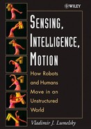
Consider a simple planar two-link arm (shown in Figure 2.1) that we will use in a few sections of this chapter. Here is some notation that we will use:
- θ1—shoulder angle
- θ2—elbow angle
- J0, J1—arm joints
- l1, l2—arm links
- m1, m2—link masses
- R—link radius
We will assume that link masses are distributed uniformly within each link. Besides axes x and y shown in the figure, imagine also an axis z perpendicular to the plane of the figure. Assume that axes of joints J0 and J1 are parallel to the axis z. (In this chapter we will not need axis z; it is mentioned here only to define the joint axes.)
The workspace of the arm in Figure 2.1 is a disk of radius (l1 + l2). Because link l1 is longer than link l2, centered at the arm's base J0 there is a dead zone of radius |l1 – l2|, no point of which can be reached by the arm endpoint b. Note that if l1 happened to be shorter than link l2, there would still be a dead zone of exactly the same radius |l1 – l2|. The arm's workspace is therefore the area sandwiched between the circles of radii (l1 + l2) and |l1 – l2|. In case the arm links are of equal lengths, the arm's workspace is a circle of radius (l1 + l2). If one or both arm joints are subject to constraints on their values, the workspace will change accordingly. This does happen with real arms; for example, the arm's joint angle θ1 may be limited to the range ±120°.
The arm's endpoint b can occupy any point in the arm's workspace. When the arm is fully outstretched, its endpoint b is at the workspace outer circle boundary; when it is fully folded, its endpoint b is at the workspace inner circle boundary. Only one arm configuration corresponds to any such point. Any other position of endpoint b in the arm workspace corresponds to two arm configurations. The second arm configuration is shown by dashed lines in Figure 2.1. If l1 = l2, an infinite number of configurations can place the arm endpoint b at the base J0, with θ2 = π.

Figure 2.1 A planar two-link arm manipulator: l1 and l2 are links, with their respective endpoints a and b; J0 and J1 are two revolute joints; θ1 and θ2 are joint angles. Both links are of the same thickness 2R. The robot's base coincides with the joint J0 and is fixed.
Position of the endpoint b can be defined in the arm workspace either by two coordinates x and y in the Cartesian plane (x, y) or by two joint angles θ1 and θ1. Hence we distinguish two representations of an arm configuration, in Cartesian space (x, y) and in joint space (θ1, θ1).
An arm with more degrees of freedom or a three-dimensional arm will result in a higher complexity of those representations.
2.1 KINEMATICS
Kinematics describes the relationship between positions, velocities, and accelerations of a set of bodies—in our case, of the robot arm links.
While we are at it, let us also define the concepts of statics and dynamics, which often go together with kinematics when describing a body's motion, and which we will address in the following sections:
Statics describes (a) the relationship between forces and torques that, say, an arm manipulator exerts on the surrounding objects and (b) the relationship between internal forces and torques at the arm links.
Dynamics describes the relationship between kinematics and statics. For example, the relationship between torques at the arm joints and link positions represents the arm's dynamics.
For trajectory planning of robot arm manipulators, kinematics is especially important. Here is one reason for that. More often than not, people prefer to command arm's positions in terms of Cartesian coordinates—in our case the two coordinates (x, y)—whereas the arm control system expects them in terms of arm's joint values—in our case the angular joint values (θ1, θ1). Inversely, if the arm somehow—say, acting upon the sensor data—arrives at some position, from the arm's joints we obtain its joint angles, and we would like to know which position (x, y) in Cartesian space they correspond to (Figure 2.1). Hence there is a need to translate from one coordinate system to the other.
Accordingly, there are two relationships between these two coordinate representations:
Direct Kinematics. Given the values (θ1, θ1), find the corresponding Cartesian coordinates (x, y) of the arm endpoint.
Inverse Kinematics. Given Cartesian coordinates (x, y) of the arm endpoint, find the corresponding joint values (θ1, θ1).
Note that if ![]() is the vector from the proximal to the distal joint of link i (Figure 2.2), i = 1, 2, then
is the vector from the proximal to the distal joint of link i (Figure 2.2), i = 1, 2, then
Direct Transformation (Direct Kinematics). From Figure 2.2, it is not hard to derive equations for the joint position, and by taking their derivatives to find equations for velocity and accelerations of the arm endpoint in terms of the arm joint angles:

or, in vector form, ![]() where the 2 × 2 matrix J is called the system's Jacobian (see, e.g., Refs. 6 and 7).
where the 2 × 2 matrix J is called the system's Jacobian (see, e.g., Refs. 6 and 7).
Acceleration:

Inverse Transformation (Inverse Kinematics). From Figure 2.2, obtain the position and velocity of the arm joints as a function of the arm endpoint Cartesian coordinates:


Obtaining equations for acceleration takes a bit more effort; for these and for other details on equations above, one is referred, for example, to Ref. 8. In general, for each point (x, y) in the arm workspace there are two (θ1, θ2) solutions: One can be called “elbow up,” while the other can be called “elbow down” (Figure 2.3a). This is not always so—one should remember special cases and degeneracies:
- Any point on the workspace boundaries—that is, when θ2 = 0 or θ2 = π —has only one solution (Figure 2.3b).
Figure 2.3 (a) In general, for each (x, y) point in the arm workspace there are two (θ1, θ2) solutions: One can be called “elbow up,” and the other can be called “elbow down.” (b) The arm's degeneracies.
- If the given coordinates (x, y) of the arm endpoint happen to lie outside of the arm workspace, then the inverse kinematics will have no solution for (θ1, θ2).
- If the arm links are of equal length, l1 = l2, then, when θ2 = π, the arm endpoint b falls into the arm origin, x = y = 0, and tan−1 (y / x) is undefined, resulting in an infinite number of solutions for the angle θ1 (Figure 2.3b).

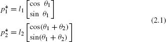
For an arbitrary rigid object in two-dimensional space, such as the rectangular object in Figure 2.4, the set of three values (x, y, θ) describe fully its configuration. The object's configuration information includes its position and its orientation. These three values are the object's three degrees of freedom (DOF), each of which can be manipulated independently. All such sets form the object's three-dimensional configuration space, or C-space.
Our two-link arm of Figure 2.1 consists of two bodies, two links, and so in principle it should have (3 + 3) = 6 DOF. But, since the arm is bound in its motion by kinematic constraints–its fixed base and the connection at its joints—it has only two degrees of freedom, angles θ1 and θ2, two DOF that fully define its configuration in space. All such sets (θ1, θ2) define the arm's two-dimensional C-space.
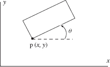
Figure 2.4 To describe the configuration of this rectangular object, an arbitrary point p is chosen on it first. Now the object's configuration is described by three values: x, y, and θ, where x and y are the Cartesian coordinates of point p.
2.2 STATICS
As formulated in Section 2.1, statics describes (a) the relationships between forces and torques that the arm exerts on the surrounding objects and (b) the relationships between internal forces and torques at the links. Statics analysis is done on an isolated link, taking into account the forces and torques contributed by neighboring links. For link i, the result of analysis is the net force fi, net torque ni, and

The force balance is
The minus in front of the second term above is due to the changed direction of the exerted force. In Figure 2.5, we have
![]()
The torque balance is (see Figure 2.5)
2.3 DYNAMICS
As defined above, dynamics describes relationships between kinematics and statics. For example, the relation between torques at the arm joints and link positions represents the arm's dynamics. Dynamics is typically a final step in deriving joint torques. Given various forces acting on the arm, one needs joint torques to realize the desired trajectory. Then by Newton–Euler equations we relate the D'Alamber force fi and torque ni (from the static equations) to the acceleration of link i [7].
Let ri be the vector from the arm base to the center of mass of link i (Figure 2.5). Take two links, link 1 and link 2, of masses m1 and m2, respectively. Then the net forces f1 and f2 acting upon the links 1 and 2 relate to the accelerations ![]() and
and ![]() of the links’ centers of mass by Newton's second law,
of the links’ centers of mass by Newton's second law,
Figure 2.5 Balance of forces and torques acting on a single link.
From these equations, accelerations ![]() of the centers of mass can be derived.
of the centers of mass can be derived.
- Let ωi be the angular velocity vector of the center of mass of link i.
- Let
 be the corresponding angular acceleration.
 - Let Ii be the inertia matrix of link i.
Then torques are related to angular velocities and accelerations by Euler's equations,
For our planar two-link manipulator shown in Figure 2.1, the torque is normal to the arm's plane. Rotary inertia through the centers of mass of links 1 and 2 are [7]
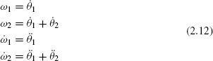
Angular velocities and accelerations are
Substituting those into Euler's equations (and taking into the account that ωi × Iiωi = 0), we obtain
Finally, Newton-Euler equations are combined with static equations [Eq. (2.8)] to produce the torques at arm joints—that is, to do inverse dynamics. After simplifications, these become (details can be found in Refs. 7 and 8)

There are three types of terms that appear in such equations. Taking as an example the above equation for n1, 2, these are:
Dynamic Torques (Terms 1, 2, and 3). These arise from the arm movement, and depend on velocities and accelerations.
Gravity Torques (Term 4). These are due to the (vertical) gravity force.
External Torques (Terms 5, 6, and 7). These are due to external forces and torques that come from the arm's interaction with other objects; they appear when the arm physically touches objects, such as in assembly or cleaning. During a free arm motion these torques are zeros.
Then there is another classification of dynamic torques, also with three types:
Inertial Torques. These are proportional to accelerations in the arm joints, and they arise from normal action/reaction forces of an accelerating body.
Centripetal Torques. These torques arise from a constrained rotation about a point, and they are proportional to the squares of joints' velocities. For example, the arm's forearm must rotate about the arm's shoulder joint, and so the centripetal acceleration is aimed at the shoulder joint along link l1(Figure 2.1).
Coriolis Torques. These torques arise from vortical forces, as a result of interaction between two rotating systems (in our case two arm links), and they are proportional to the product of joint velocities of two different links.
Notice the remarkable growth in the complexity of equations as we proceed from kinematics to statics to dynamics equations. Then there is another natural source of complexity—the arm complexity, measured by the number of robot degrees of freedom. The reader is reminded that in our example, Figure 2.1, we are dealing with the simplest two-link planar manipulator: In its analysis we started with modest kinematic equations (2.2) and (2.3) and arrived at rather complex dynamic equations in (2.14). Will the equations complexity grow as quickly with the growth in the number of robot DOF?
Indeed they will. As an example, if we write only the acceleration-related coefficients for an arm with six DOF, they form this 6 × 6 matrix (note that a great many of today's industrial robot arm manipulators have six or more DOF):
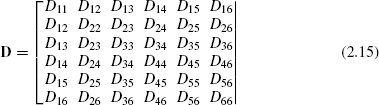
The diagonal terms in this matrix represent uncoupled terms—that is, terms caused by a single joint—and off-diagonal terms represent pairwise interaction effects for all six joints. Each such term is itself a rather complex relationship. Out of curiosity, if the very first term in the matrix above, D11, is written in full, it looks as shown in Figure 2.6 [9]. As you glance at this formula, try to imagine what the whole matrix D must look like, and imagine what kind of complexity a control system based on such expressions must involve. Consequently, all kind of simplifications are done in real-world systems when designing robot control schemes. Simplifications in equations bring, of course, imprecision, and so the design process involves carefully studied trade-offs.

Figure 2.6 The full expression for one term, D11, of the matrix (2.15).
2.4 FEEDBACK CONTROL
In the jargon of control theory, the system under control is called a plant. In our case the plant is a robot arm manipulator. In doing its job of controlling the motion of arm motors, the robot control system realizes an appropriate control law, which is the relationship between the system's input and output. For the arm control, the input is the arm's desired position(s), and the output is the arm's corresponding actual position. One can distinguish three types of control:
- Open-loop control, where the control action is applied regardless the system errors
- Linear control, in which the control law is a linear relationship
- Nonlinear control, in which the control law is a nonlinear relationship
Because there are a great number of nonlinear relationships, the term “nonlinear control” calls for further precision. Typically, the nonlinear control is more complex to realize than linear control, so a need for nonlinear control suggests that the system in question is quite complex. One finds in literature many terms related to different methods of nonlinear control: switching controls (which are further divided into a bang-bang control, duty-cycle modulation, logic control), globally nonlinear feedback mapping (e.g., saturating controls), adaptive control (with its own division into, for example, model-based reference control and self-tuning control), and so on. Both linear and nonlinear control are typically realized as a feedback-based control, as opposed to open-loop control. In a feedback control system the control law becomes a feedback control law, and is calculated based on the desired system behavior and the contemplated error (i.e. difference between the system's input and output), forming a feedback loop (Figure 2.7).
Assume that each of the two joints of our arm (Figure 2.1) has a torque motor with a unity input-to-torque conversion coefficient. As before, denote the motor torques at links l1 and l2 as n0, 1 and n1, 2, respectively. To demonstrate how the control system is synthesized, we will use an independent joint controller, called also a linear decentralized feedback law. Assume that the desired joint angles are given.
The control law we choose is of proportional-integral-derivative (PID) type, a widely used type of controller. In Figure 2.8, K is position (error) gain, L is integral (error) gain, and H is derivative (error) gain. In simple terms, the controller's position feedback component improves the speed of response of the control system; the integral feedback component ensures a steady-state tracking of the desired output; and the derivative feedback component enhances the system stability and reduces oscillation due to control.

Figure 2.7 A sketch of a feedback-based control system.

Figure 2.8 A PID control system.
Equations characterizing the control law here will come out as (see Ref. 7),
and
Steady-State Analysis. Assume that the commanded angles (θ1d, θ2d) are constant, the disturbances are constant, and the control system is stable. System stability implies that eventually all time derivatives approach zero, which, using Eq. (2.14), gives

Analysis of these equations shows that steady-state tracking will occur regardless of disturbances. Note that the value of error e1 must compensate for the value of e2 but not vice versa, which is understandable given the links' sequential connection. It can be shown that if the gains L01 and L12 are zeroes, then joint values θ1 and θ2 differ from their desired values by amounts proportional to the disturbance values and inversely proportional to the feedback gains K01 and K12. If, in turn, both gains K are zero, then the system's steady state is independent of the commands and reflects only the balance of gravitational and disturbance forces. This of course indicates the importance of the feedback.
Dynamic Stability Analysis. This is done to verify the stability hypothesis. Suppose that n2, 3 = 0, f2, 3x = 0, and f2, 3y = 0. Assume a small initial error δθ1(t),
![]()
and constant θ1d and θ2d for t > 0. Then, assuming that stability can be achieved via feedback, linearized equations in terms of δθ1(t) and δθ2(t) are written. Stability of those equations can be assessed by applying to them the Laplace transform and studying the characteristic polynomial [7]. Tests for stability are in general difficult to apply, so simpler necessary conditions are used, followed by a detail experimental verification.
2.5 COMPLIANT MOTION
When the robot is expected to physically interact with other objects, additional care has to be taken to ensure a smooth operation. Imagine, for example, that the robot has to move its hand along a straight line, on a flat surface, say a table. It is easy to program such motion, but what if the table has a tiny bump right along the robot's path? The robot will attempt to produce a straight line, effectively trying to cut through the bump. Serious forces will develop, with a likely unfortunate outcome. What is needed is some mechanism for the robot to “comply” with deviations of the table's surface from the expected surface. Two types of motion are considered in such cases:
- Guarded motion, when the arm is still moving in free space, before it contacts an object. Position control similar to the one above is used.
- Compliant motion, when the arm is in continuous contact with the object's surface. Position control and force control are then used simultaneously.
Consider an example: Let us say that our task requires the robot to grasp an object A (see Figure 2.9) that is initially positioned on top of object B1, move it first into contact with the surface of table T, then slide it along T until it contacts an object B2, and stop there. Let us assume that the grasping operation itself presents no difficulty and that the grasp is a rigid grasp; that is, for all practical purposes the grasped object A becomes the rigid continuation of the robot hand. The contact relation between object A and objects B1, T, and B2 is each a point relation and easy to accomplish. Our primary concern is the contact relation between object A and surface T during the motion of A along T. This contact relation is an external constraint on the arm's position control during this part of the path. The PID controller in our example in Figure 2.8 realizes positioning control; that is, it concerns itself only with the robot arm endpoint position (θ1, θ2) [or, equivalently, (x, y)]. In the example in Figure 2.9, such a controller would work as long as the arm moves in free space. But when the arm attempts to move its endpoint along the surface of table T, a contact constraint comes in, affecting the y component of the arm motion and acting as another “control.” With two simultaneous constraints affecting the same motion components, one from the control system and the other from a contact constraint, the system is overspecified.
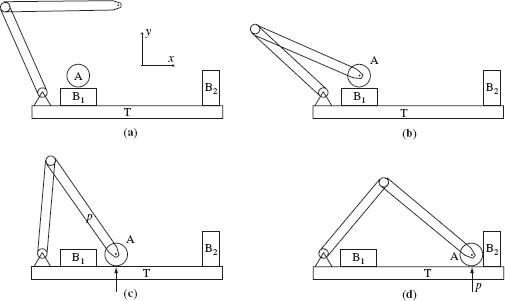
Figure 2.9 In this task, as object A is moved by the robot arm along the surface of table T, between positions (c) and (d), the control system has to maintain a compliant contact between A and T.
In other words, we have a potential conflict. Imagine that at some moment a little bump on the table will require the arm to move for an instant up and then down again. As the robot control will “insist” on moving along the straight line, the arm's positioning system will likely fail because of inconsistency of the simultaneous constraints. Besides deviations of surface T from its model, there may be a conflict due to modeling uncertainty, controller errors, and so on. We need to resolve this conflict.
The solution is to (a) add a force control at this part of the path and (b) limit the force and positioning controls so that each type never creates an overspecified system. In the task in Figure 2.9 the motion will be planned in two stages:
- A guarded motion in the y direction will be used for the part of the path in free space, namely from the arm initial position (Figure 2.9a) to grasping the object A (Figure 2.9b) to the position when object A contacts surface T (Figure 2.9c). Only position control will be used at this stage. (Since object A is immobile during the grasping operation, let us assume that such control will suffice for grasping.)
- Compliant motion control will be done during the part of motion where object A is in continuous contact with table T, between positions shown in Figures 2.9c and 2.9d. Both position and force control will be used at this stage: position control in the direction x and force control in direction y.
Here is why this control is called compliant. During this part of the path the control system will only attempt to maintain a set force pressure in the y direction. If a little bump is encountered on the table, the arm's attempt to maintain the same y coordinate as before will instantaneously develop a stronger reaction force from the table. As the arm's control measures and reacts to forces in this y direction, it will then comply, gently raising the arm enough to keep the same action/reaction forces in the y direction. As the bump is passed, the reaction force will quickly decrease, and the arm's control will move the arm endpoint a notch down, just to maintain the force at the set value.
This hybrid controller therefore has two feedback loops (see Figure 2.10): one for position control and one for force control. (Each loop may of course have its own complications; for example, each can be built as a PID controller shown in Figure 2.8.)
Remember that the controller shown in Figure 2.10 can provide a successful compliance control only specifically along the y axis, which is what is needed for the task in Figure 2.9. In reality the direction of the compliance line may differ from case to case, so for the general case a more general scheme is needed. The controller shown in Figure 2.11 can handle such cases. Its main difference from the controller in Figure 2.10 is that instead of specific matrices M1 and M2 in Figure 2.10, a generalized constraint frame 2 × 2 rotation matrix Q is used. Matrix Q describes orientation of the constraint axes. Other inputs in the scheme are as follows:
Axis s specifies the position versus control differentiation of axes,
![]()
- pd = (xdm, yd) is the desired position vector.
- fd = (fxd, fyd) is the desired force vector.
- R is the coordinate transformation of the force control loop.
- T is the coordinate transformation of the position control loop.

Figure 2.10 In the task shown in Figure 2.9, this compliance control scheme will provide position control during the motion between the positions shown in Figures 2.9a and 2.9c and will then provide force control between the positions shown in Figures 2.9c and 2.9d.

Figure 2.11 This scheme generalizes the scheme in Figure 2.10 to any orientation of the compliance line.
Suppose that the line of compliant motion forms an angle δ with the horizontal. Define a unit vector along that line as u(δ). Then:
- The position loop projection becomes u(δ)(pe · u(δ)).
- The force loop projection becomes
 .
.
These operations will be implemented properly if matrix Q is defined to align the constraint frame with the known compliance line, and vector s differentiates the directions of control loop actions:

2.6 TRAJECTORY MODIFICATION
Robot trajectories (equivalently, robot paths) are generated in many ways. For example, as explained in Section 1.2, not rarely a path is obtained manually: A technician brings the arm manipulator to one point at the time, he or she presses a button, and the point goes into the trajectory database. A sufficient number of those points makes for a path. Or, the path can be obtained automatically via some application-specific software. Either way, if the robot goes through the obtained path, it is very possible that the motion would be less than perfect; for example, it may be jerky or make corners that are too sharp. For some applications, path smoothness may be very critical. Then, the set of collected path points has to be further processed into a path that satisfies additional requirements, such as smoothness.
Depending on the application, more requirements to the path quality may appear: a continuity of its second and even third derivatives (which relates to the path smoothness), precision of its straight line segments, and so on. That is, techniques used for modifying the robot path often emphasize appropriate mathematical properties of the path curves. The path preprocessing will likely include both position and orientation information of the path. If, for example, such work is to be done for a six-DOF arm manipulator, the desired properties of the path are expected from all DOF curve components.
Common trajectory modification techniques are polynomial trajectories, which amount to the satisfaction of appropriate constraints, and straight-line interpolation.
Polynomial Trajectories (Satisfaction of Constraints). Consider an example in Figure 2.12. We want to obtain a mathematical expression for a simple path that would bring this two-link planar arm from its initial point (position) pa to the destination point pb. Positional constraints are defined by the joint angle vectors θa and θb at positions pa and pb, respectively. Here and below, θ, ω, and so on, are vectors whose dimensionality is equal to the number of system DOF; for a two-DOF robot arm, θ = (θ1, θ2), and so on. The constraints can be met by a trajectory

Figure 2.12 By constraining the path to only starting and finishing points (pa, pb), a simple straight-line path between pa and pb can be used. Adding additional constraints on velocities along the path requires going to more complex path shapes.
![]()
where function f is defined on the segment [0, 1] and converts the arm's path into a trajectory; f(a) = 0, f(b) = 1. In its simplest, the function f(t) = t produces a linear trajectory,
While geometrically a straight line is a nice trajectory, it has drawbacks: (a) A simple differentiation shows that the angular velocity of this trajectory is a constant, which means that if we want to connect together two such path segments, large (formally, infinite) accelerations will develop at the joint point of those segments. (b) From our path expression it is hard to know if the whole trajectory lies in the robot workspace. Recall that the workspace of our arm may have a circular dead zone around its base (Figure 2.1): If our straight line passes through that zone, it would mean that the path is not physically realizable.
This suggests that we may want to add other constraints to the path. Let us add constraints on velocity, ![]() . Two constraints can be met by a cubic trajectory,
. Two constraints can be met by a cubic trajectory,
In terms of its execution, this trajectory is significantly more realistic than the one in (2.20). But, it still has drawbacks: (a) The trajectory does not take into account the fact of maximum attainable velocity. (b) Accelerations (and hence torques) cannot be independently specified at the ends of the trajectory. This significantly limits our freedom in specifying the pattern of robot motion. The problem can be fixed via additional constraints, namely by specifying accelerations α at the path's beginning and end, α(a) and α(b). Now we have a total of six constraints; to meet them, a minimum of fifth-order polynomial is needed:

Straight-Line Interpolation. Achieving a straight-line motion with the arm shown in Figure 2.12 may be tricky. The reason for that is that the arm's rotating joints move links’ endpoints on circular curves. This means that we cannot have an ideal straight line, and so we need to synthesize it from curves. The more those curves and the shorter they are, the better our straight-line approximation. To accomplish this, we will calculate a number of points along the desired straight line, and will force the arm endpoint through those points. Between those guaranteed points, the arm will move as it pleases; more precisely, the arm's own control will be linearly interpolating points between our specified points. The interpolation is done in terms of joint angles, or, as we call it, in the arm's joint space (or configuration space).
To summarize, the straight-line interpolation of added points is to be done in Cartesian space, and the arm's own interpolation between those given points takes place in joint space. Assume, for example, that the θ1 and θ2 angles of points pa and pb in Figure 2.12 are ![]() and
and ![]() . This corresponds, respectively, to these Cartesian coordinates:
. This corresponds, respectively, to these Cartesian coordinates:

If we provide the robot with only starting and ending points (pa, pb) of the desired straight-line path (pa, pc, pb) (Figure 2.13), then, given the robot's joint space linear interpolation procedure, it will produce instead the curve (pa, pj, pb). The midpoints of the joint and Cartesian paths indicate the extent of deviation of the actual path from the desired path: in Cartesian terms, ![]() and
and ![]() .
.
A reasonable idea then is to further approximate the desired straight-line path by forcing the robot endpoint through more intermediate points along the straight line. This is called the bounded deviation paths technique [10]; the added points are called knots. The process starts with two knots, the initial and ending points.

Figure 2.13 Straight-line interpolation. If only starting and ending points (pa, pb) are given, the arm's control will do the rest by interpolating points in between in joint space, producing as a result the dotted curve signified by a position pj. To obtain a trajectory closer to a straight line, a set of points interpolated along the straight line, like point pc, should be given.

Figure 2.14 Forcing the robot to pass not only through the path endpoints, but also through the midpoint knot pc, decreases the deviation from the straight-line path (path 2). Adding more knots further improves the path (path 3).
If the resulting deviation is too big compared to the specified threshold, more knot points are contemplated. Intuitively, adding the path midpoint (Figure 2.14) should decrease the deviation. Hence the robot will be guaranteed to pass through three points on the straight line: the initial point, the added midpoint knot, and the ending point. Between the knots, the path is interpolated in joint space, as shown. The resulting path consists of two curves. In the bounded deviation method, the deviation resulting from each added knot is calculated, and extra knots are iteratively added to each subsegment of the path until the resulting deviation from the straight line is below the specified threshold (see paths 1, 2, and 3 in Figure 2.14).
The reality is more complex than this simple scheme may suggest. First, depending on the path's initial and ending points, in general the deviation is not necessarily symmetrical on both sides of the midpoint knot. This means that obtaining the same deviation on both sides of the path midpoint may require uneven distribution of knot points. In fact, minimizing the number of knot points that satisfy a given threshold is a complex computational problem, and so is the optimal choice of locations for knot points. Second, as Figure 2.14 demonstrates, the tangents at endpoints of two curves that meet at a knot are not equal, causing unhealthy accelerations and jerky motion when the arm manipulator is passing through knot points. Third, every arm has degenerate points where various control and computational difficulties arise [7]. For example, as discussed above (Figure 2.3), if the arm links are of the same length, l1 = l2, the arm's joint values are ill-defined when its endpoint is at the arm base. If a knot point happened to be located in the base, the inverse kinematics procedure that turns out joint angles for every proposed knot point may give solutions that are in sharp contrast with the arm's prior and future motion.
Various schemes have been considered to address those complications, such as splines between the path curve segments or approximation of the curves with more complex polynomials featuring desired characteristics.
2.7 COLLISION AVOIDANCE
Whatever robot application is considered—assembly, welding, cleaning, exploring a new planet—for the robot's own sake and for its environment, it is paramount that the robot does not bump into surrounding objects. Of the issues in robotics that we set out to review in this chapter, motion planning and collision avoidance is perhaps the most universal robotic problem. It is also the most “robotic” robotic problem: Whereas other issues and techniques considered above are common to other areas of sciences and engineering, collision avoidance—especially its branch that deals with partial input information (such as from sensors)—is the monopoly of robotics. This is true for all robots and all variations of the collision avoidance problem, from mobile robots operating in a two-dimensional surface to multilink robot arm manipulators moving in three-dimensional space among three-dimensional objects. This monopoly does not imply, of course, that the problem of motion planning is harder or easier than those other issues, but it does imply two things: (a) that robotics is a distinct discipline, with its own problems and its own methodological apparatus, and (b) that solving this problem is our full responsibility—there will be no help from other disciplines.
To avoid collisions, the robot must know something about objects that it tries to avoid. Knowledge carries a price, either in terms of sensing that is necessary to acquire it, or in terms of the amount and speed of memory the robot needs to store it, or in terms of computational power it needs to process this knowledge. In fact, a complete information about the robot workspace is usually of tremendous volume and tremendous complexity and can tax the most advanced computers. The less knowledge about its surroundings the robot needs for successful collision avoidance, the more attractive the corresponding strategy. In this sense, collision avoidance is an information-theoretical problem.
Once the robot knows enough about objects in its surroundings, it has to figure out how to avoid those objects, while not jeopardizing its primary task. If moving my hand to replace a book on the shelf is about to cause my elbow to bump into a nearby file cabinet, there are great many ways to avoid the collision—I just need to think about this. I may think hard and slowly, or I may react instantly based on my instincts and experience; either way, I am using my intelligence to avoid collision. This example suggests that collision avoidance is a problem of artificial intelligence.
Collision avoidance relates to moving in space among objects; hence it is not surprising that collision avoidance is heavily tied to concepts and techniques from geometry and topology. Objects in the robot workspace that are to be avoided may be static, or they may be moving. Moving obstacles add to complexity of the collision avoidance problem. Some techniques are amenable to moving obstacles and some are not. While this book addresses static obstacles, we will stress the applicability of some strategies to moving obstacles. Most of the time we will limit the discussion to the effects of kinematics, leaving out the robot dynamics. Some collision avoidance problems with dynamics are considered in Chapter 4.
The information-theoretical base of the collision avoidance problem gives rise to one classification of motion planning strategies that turns out to be very productive. The classification divides all approaches into two groups, each presenting a distinct paradigm:
- Motion planning with complete information, also called in literature the Piano Mover's model or off-line planning approach. Here the path is computed all at once before the motion starts; in principle, an optimal path can be found in this way.
- Motion planning with incomplete information, also called sensor-based motion planning or on-line motion planning, or path planning with uncertainty, or the Sensing–Intelligence–Motion (SIM) paradigm. Here the decision-making is done continuously as the robot moves along, based on on-line information, such as from sensors. By its very nature, an optimal solution is ruled out in this formulation.1
A simple relation governs the choice of one or the other approach in robot applications. If all the information necessary to produce the desired path is available beforehand one would want to produce the path beforehand and would hence choose the Piano Movers approach. On the other hand, if the information happens to be coming in real time from robot sensors, and thus there is always uncertainty about the robot's surroundings, one is forced to turn to the second approach, SIM.
In other words, as a rule, only one approach applies to a given task. Consider, for example, a maze-searching task (called also a mouse-in-the-labyrinth problem). One starts at some starting point S inside the labyrinth and attempts to reach some target point T, also in the labyrinth.2 Imagine we have in our possession complete information about the labyrinth. We can feed these data into the computer, produce the bird's-eye view of the maze, and study the problem in great detail using this map. We can investigate different paths between points S and T, figure out the optimal (shortest) path, and so on. This is planning with complete information, and the Piano Mover's model should be the preferred approach.
On the other hand, if all of a sudden you find yourself in a maze, at any given moment you would see only the surrounding walls of the maze and perhaps remember a few corridors that you have just passed. You do not know what is ahead; input information is scant; what you learn comes from your sensors. Any movement, including the unfortunate deviations into dead end corridor appendices, becomes a part of the path. Doing anything approaching an optimal path is of course out of the question. Here you deal with incomplete information and produce the path as you go. This is planning with incomplete information, and so you need to turn to the SIM techniques.
Since robot motion planning is the topic of this book, in Sections 2.8 and 2.9 we will further explore differences between these two paradigms for motion planning, the Piano Mover's model and the Sensing–Intelligence–Motion model.
Provable Versus Heuristic Algorithms. Another important distinction between algorithms is between provable (other terms: nonheuristic, exact, algorithmic) and heuristic approaches.
A provable motion planning algorithm is one for which there is a guarantee that if a path between the starting and target points exist, the algorithm will find one in finite time and without an exhaustive search—or else will conclude in finite time that there is no path if such is the case. We then say that the algorithm converges. To obtain such a guarantee, people go through the trouble of proving the algorithm convergence. An algorithm itself should allow such a proof; for example, the so-called “common sense” strategies—we call them heuristic algorithms—do not allow a proof of convergence and are not likely to be convergent.
Whereas for some applications, having a guarantee of convergence may be a moot point—as, for example, when the user's knowledge or intuition pretty much replaces it—for more complex cases, seeking convergence reflects more than a love for academic purity. As we will see in Chapter 7, in complex problems—most motion planning problems with robot arm manipulators fit this category—human intuition is not a good advisor. If, while operating under some reasonably sounding algorithm with unproven convergence, the robot fails to find a path, the failure may simply mean that feasible paths do exist but the algorithm has missed them. A guarantee of convergence then becomes a very practical issue.
2.8 MOTION PLANNING WITH COMPLETE INFORMATION
In this type of motion planning, input information is processed before the actual motion starts. This means that the input information must exist beforehand.
The model with complete information is formulated as follows.3 Given a solid object (robot), or a combination of solid objects, in two- or three-dimensional space, whose size, shape, and initial and target position and orientation are fully described, and given a set of obstacles whose shapes, positions, and orientations in space are likewise known, the task is to find a continuous path for the object from the initial to the target position while avoiding collisions with obstacles along the way. An important assumption used in the model is that the surfaces of the moving object and the obstacles are algebraic or semialgebraic. This guarantees a final description of the input data. In some works a stricter requirement of planar surfaces is imposed.
Because complete information about the problem is assumed, the whole operation of path planning is a one-time, off-line operation. The main difficulty is not in proving existence of algorithms that would guarantee a solution (they obviously exist), but in assessing the problem complexity and obtaining a computationally efficient procedure. Reaching a solution means either finding a path or concluding in finite time that no path exists. Since a solution is always feasible, cases of arbitrary complexity can in principle be considered. Another apparent advantage of dealing with complete information is that various optimization criteria—finding the shortest path, or the minimum-time path, or the safest path, and so on—can be introduced easily.
Historically, Piano Mover's approach strategies were the first to come, starting in late 1960s. Most of the people who formulated the problem of robot collision avoidance were computer scientists. For them, collision avoidance was a purely computational problem, and the question of handling input information boiled down to a search in the database that contained that information. They often perceived sensing, partial information, uncertainty, control, and all such issues as small conceptual bumps that only interfered with the beautiful computational problem in hand. By the late 1980s, the area became one of the richest and popular areas in computational geometry. Hundreds of planning algorithms with complete information have been published; the problem's computational complexity has been studied in depth, and ingenuous ways of dealing with it were reported [11].
By the late 1980s and early 1990s, it was slowly becoming clear that the domains to benefit from the Piano Mover's approach related not so much to robotics as to some other specialized areas where “clean” information would be available. One would read less about robots and more about a strategy for a quick extraction of an assembly unit from an aircraft engine without disassembly of the whole engine; or of optimizing the design of a car door opening so as to simplify the installation of car seats; or of finding the route that a protein molecule follows when folding into a complex shape during the DNA mapping of proteins. Note that in these cases the complete aircraft engine database, or a complete car body database, or a complete database of the protein geometry would be available beforehand.
The way the Piano Movers strategies proceed is as follows. Before the motion planning proper is attempted, the task's configuration space (C-space) is calculated. Assume for now that the robot—or, in general, an object for which the motion planning task is contemplated—is a rigid body moving in two-dimensional (2D) space (see object A, Figure 2.15a). In C-space the robot shrinks to a point, whereas the surrounding objects—we call them obstacles—are grown accordingly, to compensate for the shrinking robot.
Free subspace of C-space is the complement to the grown obstacles. Any path that lies in a continuous subset of free space is a physically realizable path for object A. In order to decide which areas of free space are connected and which are disconnected, and whether and how two patches of free space can be passed from one to another, an additional intermediate structure is built, the connectivity graph of C-space. A path is then declared to exist if the start and the destination nodes on the connectivity graph are connected [11, 13].

Figure 2.15 (a) The task is to move object A from its starting position S to the target position T, while keeping its orientation constant. (b) The C-space of task (a): Object A shrinks to a point, and obstacles O1 and O2 grow accordingly. Notice a simple fact: For A to be able to pass between O1 and O2 in the physical space (a), the grown obstacles in (b) must not overlap.
If the robot's orientation in space is maintained constant for the duration of its motion, the computation of C-space is relatively easy. If, in addition, the robot and obstacles are 2D polygons, then the grown obstacles are also polygons, though not necessarily with the same number of edges as in the original polygons (Figure 2.15b).
If, however, the robot orientation is allowed to change during the motion then, the C-space for a 2D workspace becomes a 3D space of parameters (x, y, θ), where θ is the robot orientation angle (Figure 2.16a). In this case, even the original polygonal robot and/or obstacles produce nonpolygonal and, in general, nonlinear grown 3D obstacles in C-space (Figure 2.16b). As complexity of the robot and obstacles increases—for example, in cases with 3D multilink arm manipulators and nonpolygonal obstacles—computation and proper representation of the C-space becomes an exceedingly difficult task.
The computational complexity of the problem is measured in the Piano Movers model in terms of the connectivity graph's structure. Overall, the computational price for dealing with perfect information and for the said advantages—optimal paths and, in principle, solutions for cases of arbitrary dimensionality—is high. Today many reasonable-size problems still cannot be approached.
From the application standpoint, unless there is a reason to believe that obstacle boundaries are algebraic (which would squarely mean that we are dealing with man-made objects), an appropriate approximation of the robot workspace has to be performed before the connectivity graph can be calculated. The approximation itself necessarily depends on considerations that are secondary to the path planning problem. One may specify, for example, the accuracy of presenting actual obstacles with polygons, or—a different criterion—one may put a limit on the computational cost of processing the resulting connectivity graph.
The approximation process can introduce significant computational costs of its own. John Reif has shown that approximation of nonlinear surfaces with linear constraints itself requires time exponential in the prescribed accuracy of approximation [14]. Also, the space of possible approximations is not continuous in the approximation accuracy; that is, a slight change in the specified accuracy of approximation can cause a dramatic change in the number and positions of nodes of the approximated surfaces and eventually in the generated paths.
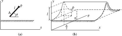
Figure 2.16 (a) When robot orientation is added to a 2D task, the (b) resulting 3D C-space of parameters (x, y, θ) is nonlinear, even if the original robot and obstacles are polygons. Here the “robot” A is a line segment of length l, and the obstacle is a horizontal “table” line.

Figure 2.17 Which of the three obstacles, A, B, or C, would be easier to pass around?
Measuring the computational burden in terms of complexity of the connectivity graph may create peculiar situations where the derived computational complexity of a given task contradicts our intuitive notion of problem complexity. Consider, for example, a circular obstacle A in Figure 2.17. Assume that the motion planning algorithm that we plan to use requires polygonal obstacles. Then, obstacle A is first approximated—say, by one of the polygons B or C in Figure 2.17.
Now, according to Piano Mover's algorithms, planning a path around obstacle C is computationally more difficult than planning a path around the obstacle B, because of the greater number of nodes in C. Moreover, in the limit, increasing the accuracy of polygon approximation takes the computational burden to infinity. But, from the human and from the robotics control viewpoints, walking around the circle A is actually easier than walking around obstacles B or C, because the latter require special decisions at the corners of the obstacle. Also, from the dynamics standpoint, there is an undesirable sharp change in the velocity vector at the corners of obstacles B and C. One can, of course, solve this specific example by including circular objects in the list of those allowed by the algorithm, but this will only shift this discussion to some other shapes.
For more detail on the Piano Mover's model, the reader is referred to the literature. The model's computational complexity for cases of rigid or hinged bodies has been studied extensively. The problem was shown to be computationally prohibitive [15–17]. A 2D case has been studied in Refs. 18–20. Cases where objects to be moved are polygons (polyhedra) or discs (spheres) moving amidst polygonal (polyhedral) obstacles are considered in [15, 18, 19, 21–23]. The first attempt to study the case of moving an object with a number of free-hinged links was initiated in 1968 by Pieper [24], in the context of motion planning for robot arm manipulators. Exact algorithms for this problem have been described [15, 16, 20], as have various heuristics (e.g., see Refs. 25 and 26).
The computational complexity of the problem was first reported by Reif [15], who showed that the general Piano Mover's problem is PSPACE-hard. He also sketched a possible solution for moving a solid object in polynomial time, by direct computation of the “forbidden” volumes in spaces of higher dimensions.4 Reif also demonstrated that even the preliminary operation of approximating the robot workspace with a specified accuracy carries a high computational cost. Schwartz and Sharir [18] presented a polynomial-time algorithm for a 2D Piano Mover's problem with convex polygonal obstacles. It has been shown in a number of works (e.g., Lozano-Perez and Wesley [27]) that the process of moving in the task's configuration space carries additional computational costs. In general, even if the original obstacles are polyhedral, obstacles in the configuration space have nonplanar walls. In order to keep the problem manageable, various constraints are typically imposed.
Moravec [28] considered a path planning algorithm for a mobile robot moving in two dimensions, with the robot presented as a circle. In his treatment of a 2D path planning problem with a convex polygonal robot and convex polygonal obstacles, Brooks and Binford [29, 30] used a generalized cylinder presentation to reduce the planning problem to a graph search. A generalized cylinder is formed by a volume swept by a cross section (in general, of varying shape and size) moving along the cylinder axis, which in turn can be some spine curve.
The version of the Piano Movers problem where the robot can consist of a number of free-hinged links is more difficult. On the heuristic level this version was started by Pieper [24] and further investigated by Paul [31]. Both were attracted to the problem's obvious relation to control of robot arms with multiple degrees of freedom. Later, new approaches for this version have been considered in Refs. 16 and 20. The most general (although very expensive computationally) algorithm for moving a free-hinged body was given by Schwartz and Sharir [16]. The technique is based on the general method of cell decomposition; the robot and obstacles are assumed to be limited by algebraic surfaces. A more economical (but still prohibitive for many practical tasks) algorithm for the general case was reported by Canny [32]. A variety of special cases shown to lead to simpler algorithms were described by Hopcroft et al. [20].
2.9 MOTION PLANNING WITH INCOMPLETE INFORMATION
By the mid-1980s it became clear that the inherent uncertainty of a realistic robot environment and the subsequent need for real-time sensing called for a paradigm of motion planning that would fundamentally differ from the Piano Mover's paradigm. It was further realized that uncertainty and sensing were not some small irritating “engineering details” but major factors in the theoretical foundation of motion planning algorithms. As it turned out, uncertainty and sensing became the very center around which the new paradigm would be built. The result was the theory and practice of robot motion planning with incomplete information, or the SIM (Sensing-Intelligence-Motion) paradigm.
The information-theoretical (or uncertainty) aspect of the problem at hand points to connections with other fields. In general terms the problem of sensor-based motion planning can be seen as one of reaching a global goal using local means. Thus presented, it becomes a fundamental problem, various formulations of which have been studied in a number of areas. For example, in game theory (differential games and macroeconomics; see, e.g., Ref. 33) one is interested in conditions under which individualistic interests of many agents can result in predictable behavior of the whole group. In works on collective behavior, algorithms are designed whereby a group of individuals can organize a unified action at a specific moment based on local interaction only, without centralized control. In the Firing Squad Problem [34], soldiers are requested, using only pairwise communication, to agree on a moment when they fire all at once. In computer science, local operations are used to study database searches with uncertainty [35]. In geometry, attempts have been made to prove theorems of Euclidean geometry using local input information [36]. The difficult question of the relationship between uncertainty and algorithm complexity has been tackled in Ref. 37.
While some considerations, such as the importance of computational properties of their methods, still served as a bridge between the Piano Mover's and SIM paradigms, with time many divergent issues made them harder and harder to compare. One such issue is of course the SIM's favoring continuous computation over the Piano Mover's one-time computation. The other issue is the option of optimal solutions inherent in the Piano Mover's model but inherently impossible in the SIM model—not because of inferior algorithms, one should add hastily, but because of the inherent lack of relevant input information. Still another issue, as we shall see, is the difference in how both models deal with algorithm complexity (again, not because of algorithms' specifics but because of the nature of uncertainty). What counts in the Piano Mover's model is the complexity of the whole robot scene. In contrast, what counts in the SIM model is the amounts of robot's “wandering” in the scene and visits to some previously visited places in the scene. Let us consider these and other factors in more detail.
The SIM paradigm formulation includes an assumption that information about the robot's surroundings comes in real time, usually from its sensors. Except perhaps for some exotic sensors (“X-ray” vision and the like), sensory information is of local, rather than global, nature—sensors tell one something about their surroundings. In the SIM algorithms that will be developed in the following chapters, the only input information available to the robot at all times is its own coordinates and those of the target location. As the robot starts moving, new information appears from its sensors.
To exhaust the extreme case and demonstrate the algorithm completeness, we will start the algorithm development with the “ultra-local” tactile sensor. That is, the robot learns about an obstacle's presence only when it touches it physically. Later we will extend the resulting strategies to the case of proximal sensing, such as vision.
In motion planning with uncertainty, the guarantee of a solution—which is predicated on the algorithm convergence—should be distinguished from the guarantee of the solution optimality. As we will see, the former is feasible even in a very complex environment, whereas the latter is not feasible with the best of algorithms. No optimality of the solution can be promised even if only a small piece of information about the environment is missing. One's path that may look ill-conceived with hindsight may not have been planned any better with the information available at the time. A person visiting a big building for the first time should not be blamed for wandering around in search of a desired office. We are also familiar with similar patterns taking place in time, rather than in space. If a stock market investor had tomorrow's information, he would have become rich quickly. Given that he doesn't, his actual behavior may look less than optimal a few days or weeks later.
If the path optimality is not a good criterion, how does one judge the performance of a motion planning algorithm with uncertainty? Given the real-time nature of SIM algorithms, they are expected to allow reasonably fast processing and to produce “reasonable quality” paths. The first requirement is easier to grasp: It is clear that a robot cannot afford to spend a minute on calculation of a step of a continuous path that takes 20 ms to execute. For the algorithm performance, standard complexity theory performance estimates call for lower and upper bounds on the problem itself and on specific algorithms, as a function of the problem complexity.5
What is a “reasonable” path? In general, how do we assess algorithms' performance? The problem complexity is presented in complexity theory as a function of the number of elements in the problem at hand. In our case the scene complexity cannot be assessed in these terms because it may never be known, and even the notion itself of the scene complexity is very unclear. Unstructured environments typically include “shapeless” objects: Representing them with analytical entities is difficult because, again, objects are not known in advance.
Doing this would be also pointless because this representation is unrelated to what is easy or difficult for SIM algorithms. What we may think of as a complex shape may be as easy or difficult for a SIM algorithm as a simple shape. As another option, one might argue that because in any realistic system the robot moves in discrete steps, those steps might be used to build a real-time objects' approximation. This choice is also hard to defend because the size and number of those steps may differ from one robot control system to the other. What is left is to estimate the quality of the path itself that the algorithm generates.
A better measurement of algorithm efficiency in the case with uncertainty is a function tied to the length of paths that the algorithm generates. More precisely, the criterion measures the extent of the robot's “wandering” under a given algorithm: It assesses the maximum number of times, n, of the robot's retracing some segments of its path. When comparing algorithms, this upper bound will actually be independent of the length of paths, in the following sense. We can say, for example, that the algorithm A is better than the algorithm B because their n numbers are 2 and 3.5, respectively. That is, under algorithm A the robot will visit the same piece of its path at most twice, whereas under algorithm B it can visit a piece of its path at most 3.5 times.
One inherent weakness in algorithms with incomplete information is that the problem dimensionality cannot be made arbitrarily high. This drawback, again, comes from the nature of dealing with uncertainty, not from the lack of good algorithms. Consider, for example, a point robot flying in the three-dimensional space, like a fly. If the robot meets an obstacle, it has an infinite number of possibilities for passing around it. Given the robot's limited knowledge about the scene, its difficulty is unsurmountable: While good sensing will often help, in the worst case the robot may have to search an infinite number of paths to find one acceptable path. Luckily, for the cases of practical interest—mobile robots moving on a 2D surface and 3D arm manipulators—the situation is inherently easier.
The lack of information about the robot environment dictates a shift of emphasis in the SIM paradigm from objects' geometry to their topology. Relying on geometric properties of objects, as in the Piano Mover's model, would make SIM algorithms too brittle. We will see that a more sensible approach is to rely on the scene's topological properties; this allows one to tolerate uncertainty in objects' geometry. Hence there is a corresponding shift in the SIM paradigm from computational geometry tools to those from topology.
There are two other factors that have not been mentioned yet and that are often neglected in both the Piano Mover's and SIM algorithms. One is the robot dynamics. If the robot is heavy and moves relatively fast, no strategy in the world will prevent it from collisions unless this strategy is capable of handling the relation between the robot dynamics, its speed, its sensing, and of course the robot's goal. A submarine cannot stop on a dime: Its motion control system has to process an impending collision in advance; how it avoids collision will also depend on what it plans to do next. In other words, a realistic motion planning system may well need to account for the system dynamics. This factor will be considered in Chapter 4.
The second factor relates to the robot's shape and dimensions. There is always a question of how an algorithm that assumes a point robot will work for a real robot with blood and flesh. A small robot can pass where a big robot will not. One can pass a narrow corridor with folded arms, but won't be able to do it with outstretched arms. Besides accounting for the robot dimensions, this also suggests the effect of robot kinematics on motion planning.
We will see in the next section that the first serious approaches to the motion planning problem started with an abstract problem of searching a graph. The major actors in the events had no idea that their work would be a contribution to robotics. Some formulated it as a maze-searching problem, in a rather narrow way, where a maze is defined as something that would be practically equivalent to a graph. We will see in the sequel that something is lost when replacing a scene by a graph: A graph may lose some information from the original problem. Below we first review those first graph-searching approaches, switching then to the proper prior work on robot motion planning.
2.9.1 The Beginnings
Leonhard Euler, perhaps the most famous mathematician of all time, was born on April 15, 1707, in Basel, Switzerland, and spent most of his career, between 1727 and 1741 and then from 1766 until his death on September 18, 1783, in St. Petersburg, Russia, holding a prestigious position of academician—that is, a full member of Russian Academy of Sciences. As his fame grew, in 1733 he succeeded Daniel Bernoulli to the chair of mathematics in the Academy. It was at this first period of his St. Petersburg career, in 1736, that Euler proposed and solved a problem that was to become famous under the name Köenigsberg Bridge Problem. This work marked the beginning of two new mathematical disciplines, graph theory and topology. It also gives an important insight into the robot motion planning problem.
The city of Köenigsberg (called today Kaliningrad and being a part of Russia) was divided into two parts by the Pregel River, with the Island of Kneiphof in the middle. Seven bridges connected the island with the rest of the city (see Figure 2.18a). The question posed to Euler by the city's residents was this: Can a pedestrian, starting at some point, pass all seven bridges and return to the starting point so that he will traverse each bridge exactly once?
To find the solution for the puzzled residents of Köenigsberg, Euler decided to first reduce the problem to an equivalent abstract problem. In a leap of imagination, he said that the shapes and dimensions of the masses of lands that the bridges connect (A, B, C, D, Figure 2.18a) are immaterial for the problem. What matters are the connectivity properties of the scene, what today we would call the topological properties of space. This argument became the beginning of the discipline of topology. Euler denoted the land masses as vertices of a diagram, and he denoted the bridges as edges connecting the vertices (Figure 2.18b); hence the graph theory was born.

Figure 2.18 The Köenigsberg Bridge Problem.
The path that the Köenigsberg citizens wanted is called today a Euler path, and the graph it corresponds to is called a Euler graph. Define the number of edges incident to a graph vertex as the vertex degree. In today's formulation the related theorem sounds as follows:
Theorem 2.9.1 (Euler [38]). A finite graph G is an Euler graph if and only if (a) G is connected and (b) every vertex of G is of an even degree.
In the case of distinct starting and final points (which is the situation typical for the robot motion planning problems), exactly two vertices must be of an odd degree. For the Köenigsberg Bridge Problem the answer to the question posed to Euler is therefore “no” because all the vertices on the corresponding graph are of an odd degree.
As we saw above in the role of connectivity graphs in the Piano Mover's model, graph theory became an important tool in designing motion planning strategies with complete information. We will see in Chapters 3, 5, and 6 that topology became a no less important tool in sensor-based motion planning.
Neither Euler nor many of his followers asked explicitly what information about the scene was available to the traveler in the Köenigsberg Bridge Problem.6 It was implicitly assumed that the traveler had complete information.7 What if he didn't? What if at any moment of the trip the traveler's knowledge was limited by what he could see around him plus whatever he remembered from the path he had traversed already? What if this more realistic situation took place?
No live creature counts on knowing in advance all the objects on its journey, or calculates the precise path in advance. Algorithmically, the question about available input information puts the problem squarely into the domain of sensor-based motion planning, presenting it as a maze-searching problem. Clearly, even if the Köenigsberg bridges made a Euler graph, and if the traveler had no picture as in Figure 2.18, we can doubt that he would pass every bridge exactly once, except perhaps by sheer chance. If not, what would be the traveler's performance—say, with the best algorithm possible? Can a strategy be designed that will guarantee at least passing the whole graph when one starts with a zero knowledge about it? If so, how about doing it in some reasonably efficient manner? We will return to these questions later in this chapter.
This branch of motion planning—which can be formulated as moving in a graph without prior information about it—started long before Euler. Since the times of Theseus of Athens, people had great interest in labyrinths (mazes). After Theseus slew the Minotaur, he used the thread of glittering jewels given to him by Ariadne to find his way in the passages of the Labyrinth of Knossos. Many medieval churches and castles in Europe had mazes in their gardens or as inside mosaics on the floor. Many mazes are built even today for public amusement and contemplation. Some labyrinth builders tried to emulate the famous labyrinth of the Chartres cathedral in France; one Chartres-type labyrinth appears in the Grace Cathedral in San Francisco. Even Washington, D.C., the United States capital, has its own tiny labyrinth in the small pretty St. Thomas Parish Park located in the heart of Dupont Circle.
Most collections of puzzles contain labyrinth problems. A “Bible” of labyrinths that is monumental in coverage, unique, and marvelously written is the book by Hermann Kern, Through the Labyrinth: Designs and Meanings over 5000 Years (originally published in Germany in 1983 [40] and translated into English in 2000 [41]).
A simple labyrinth is a set of corridors lying in the plane and connected in intricate ways. A labyrinth can be described by a graph whose edges represent corridors and vertices (vertices are the points where the corridors meet). Figure 2.19a shows the famous labyrinth in the garden at Hampton Court in London; the corresponding graph is shown in Figure 2.19b.
The problem is as follows: Given two points in a labyrinth, start S and target T, can a method be designed that would guarantee a path from S to T ? It is usually assumed that the traveler has no beforehand knowledge about the labyrinth and has a way to mark the corridors and corridor intersections. In graph terms, this is a graph-searching problem: Given two graph vertices S and T, design a method to generate a path from S to T if one exists.
A general maze does not have to have explicit corridors and intersections. An arbitrary scene with obstacles presents a kind of maze. Any motion planning task for a robot in the plane can therefore be seen as a maze search. Such tasks can be naturally reduced to a graph search. Consider the scene in Figure 2.20a. Suppose a point robot plans to start at point S and reach point T. Suppose the robot knows its own location and that of T but has no beforehand knowledge about obstacles on its way. Then, it would be reasonable for the robot to take the shortest route to T, a straight line. Let us call this line the Main line, or M-line. If M-line happens to be free, the robot reckons, this would be the fastest route to T; if there are obstacles on the way, it will deal with them somehow. (The notion of Main line will appear often in the following chapters.)
Together with the scene, this strategy defines a graph that, although unknown to the robot, relates to the physical reality. Vertices of the graph are points S and T, as well as intersection points between M-line and obstacle boundaries; its edges are segments of M-line outside the obstacles and segments of obstacle boundaries (Figure 2.20b). The graph is called the connectivity graph of the maze. It has a simple structure: Vertices S and T are of degree one, and all other vertices are of degree three. Note that since each vertex has an odd number of edges incident to it, this is not a Euler graph, and so traversing the whole graph will result in at least some edges being traversed more than once. The graph can be easily transformed into a Euler graph—for example, by replacing with two segments each M-line segment that connects two obstacles.

Figure 2.19 (a) The Hampton Court labyrinth; (b) the corresponding graph.
If all mazes can produce connectivity graphs of this particular structure, one may wonder if this property can warrant algorithms with better performance than algorithms for a general graph —that is, one with an arbitrary degrees of vertices. This raises still another question: Can mazes produce graphs with an arbitrary degrees of vertices? At first glance, the answer is yes: Many corridors in a maze can meet in the same spot, so connectivity graphs produced by realistic mazes must be general graphs.
Notice, however, that this argument ignores the fact that mazes appear in a continuous plane, not in some discrete domain where only one path exists in a limited space such as a corridor. Spaces between obstacles leave many options for moving in them. Even a corridor has a finite space between its walls: One can walk, for example, in one direction along one wall and walk back along the other wall; or one can move in a zigzag manner between walls. That is not what we represent by a graph; instead we want a “minimum” graph that describes the maze, and hence graph edges are maze walls and M-line segments, and vertices are points where those segments meet. This means that all physical mazes can be reduced to a graph with the maximum vertex degree three (see Figure 2.21). Hence we are back to our first question: Does this special graph structure promise algorithms whose performance is better than that of algorithms for general graphs?

Figure 2.20 (a) A typical motion planning task. (b) The corresponding graph.

Figure 2.21 (a) In spite of the four-way corridor around points b, c, each vertex b, c in the corresponding connectivity graph (b) is of degree three.
Denote the length of M-line as D, denote its segments outside the M-line as di, and denote the segments of obstacle boundaries cut by the M-line as pi (Figure 2.20a). Those lengths can signify weights on the graph edges. Then the total “length” of the graph is no more than D + Σi pi.
The first systematic procedure for solving maze problems—in fact, for covering a general graph—seems to be the one suggested by Wiener in 1873. His algorithm is as follows:
Wiener's Algorithm: Starting at point S, proceed along the graph edges as far as possible, selecting at each vertex an edge that has not been traversed before. At a vertex where such motion is no longer possible, retrace the sequence of edges until you arrive at a vertex with some unused edges.
Clearly, Wiener's method presents a version of what is called today an exhaustive search. One will also recognize in this algorithm a geometric version of the “width-first” procedure that appears in many textbooks in computer science. The procedure does guarantee covering all edges of the graph, but it will produce many repetitive visits to the same vertices.
Does an algorithm have to be that inefficient? For example, how about the following simple algorithm found in children stories? “Keep your left hand on the wall as you walk, and you will eventually get out of the labyrinth.” This naive procedure will only work if all the walls in the labyrinth are connected. Clearly, if one keeps the hand on the wall that is a part of an island inside the labyrinth, one will walk in the labyrinth forever.
To understand the limits of achievable performance of algorithms with incomplete information, let us see first what that limit is for algorithms with complete information, for a general graph.
Theorem 2.9.2 (Ore [42]). In a finite connected graph, it is always possible to construct a cyclic directed path passing through each edge once and only once in each direction.
This promises a much better performance than in Wiener's algorithm, but is such performance feasible for an algorithm with incomplete information? The positive answer was given in the method by Tremaux (reported by Lucas in 1892 [43]). It was shown in 1895 by Tarry [42, 44] that the same result can be obtained in a more economical way. In Tarry's algorithm, called Tarry's rule, for a given graph, when the point robot arrives at a vertex υ, the following input information is assumed: (i) the subset of those edges incident to υ that the robot traversed before when leaving υ —that is, those edges that were traversed in the direction pointing away from υ; (ii) the entrance edge via which the robot first arrived at υ. The procedure is very simple:
Tarry's Rule:
- Upon arrival at υ, continue via an edge (υ, υ′) that was not yet traversed in the direction of υ to υ′.
- Choose the entrance edge as a last resort.
Under Tarry's algorithm, assuming that the start and target vertices are distinct and there exists a path between them, the target vertex is guaranteed to be reached, and every edge will be traversed exactly twice, once in each direction, with the exception of the two edges incident to the start and target vertices, which will be traversed once each. Using our terminology, the upper bound on the length of paths generated by the algorithm is as follows:
Theorem 2.9.3. For any finite maze, Tarry's algorithm will generate a path of length P such that
where D is the length of M-line, and pi are perimeters of obstacles in the maze.
Finally this gives us an answer to our question above: What performance can be expected for an unknown Euler graph.
It took a long time, over 70 years, for the next improvement to come. In 1970, Fraenkel proposed a more economical algorithm [45, 46]. Though it has the same performance as Tarry's in the worst case, it performs better if the robot is lucky with the maze; then, some or even all graph edges may be traversed just once. Fraenkel's algorithm is more complex that Tarry's. It makes use of a counter, which is set to zero at the start vertex. The algorithm operates as follows:
Fraenkel's Algorithm:
- Whenever one arrives at a vertex not visited before, increase the counter by 1.
- When arriving at a vertex υ such that before entering it there was at least one edge incident to it that was not traversed before, and upon arrival at υ there remains at most one such edge, decrease the counter by 1.
- As long as the counter is positive, the tour is conducted according to the Tarry's algorithm, except, whenever possible, an edge not traversed before is preferred to an edge already traversed.
- As soon as the counter contains zero, leave all edges via their entrance edges.
The accompanying theorem, whose proof is relatively involved, is derived for the case when the start and target vertices coincide. The theorem states that under Fraenkel's algorithm the target vertex is guaranteed to be reached if reachable, and every edge will be traversed at least once but never more than twice, once in each direction. Using our terminology and the M-line concept, the upper bound on the length of paths generated by the Fraenkel's algorithm is as follows:
Theorem 2.9.4. For any finite maze, Fraenkel's algorithm generates a path of length P such that
where D is the length of M-line, and pi are perimeters of obstacles in the maze.
In other words, the worst-case estimates of the length of generated paths for Trumaux's, Tarry's, and Fraenkel's algorithms are identical. The performance of Fraenkel's algorithm can be better, and never worse, than that of the two other algorithms. As an example, if the graph presents a Euler graph, Fraenkel's robot will traverse each edge only once.
2.9.2 Maze-to-Graph Transition
It is interesting to note that until the advent of robotics, all work on labyrinth search methods was limited to graphs. Each of the strategies above is based solely on graph-theoretical considerations, irrespective of the geometry and topology of mazes that produce those connectivity graphs. That is why constructs like the M-line are foreign to those methods. (M-line was not of course a part of the works above; it was introduced here to make this material consistent with the algorithmic work that will follow.) One can only speculate with regard to the reasons: Perhaps it might be the power of Euler's ideas and the appeal of models of graph theory.
Whatever the reason, the universal substitution of mazes by graphs made the researchers overlook some additional information and some rich problems and formulations that are relevant to physical mazes but are easily lost in the transition to general graphs. These are, for example: (a) the fact that any physical obstacle boundary must present a closed curve, and this fact can be used for motion planning; (b) the fact that the continuous space between obstacles present an infinite number of options for moving in free space between obstacles; and (c) the fact that in space there is a sense of direction (one can use, for example, a compass) which disappears in a graph. (See more on this later in this and next chapter.)
Strategies that take into account such considerations stay somewhat separate from the algorithms cited above that deal directly with graph processing. As input information is assumed in these algorithms to come from on-line sensing, we will call them sensor-based algorithms and consider them in the next section, before embarking on development and analysis of such algorithms in the following chapters.
2.9.3 Sensor-Based Motion Planning
The problem of robot path planning in an uncertain environment has been first considered in the context of heuristic approaches and as applied to autonomous vehicle navigation. Although robot arm manipulators are very important for theory and practice, little has been done for them until later, when the underlying issues became clearer. An incomplete list of path planning heuristics includes Refs. 28 and 47–52.
Not rarely, attempts for planning with incomplete information have their starting point in the Piano Mover's model and in planning with complete information. For example, in heuristic algorithms considered in Refs. 47, 48 and 50, a piece of the path is formed from the edges of a connectivity graph resulting from modeling the robot's surrounding area for which information is available at the moment (for example, from the robot's vision sensor). As the robot moves to the next area, the process repeats. This means that little can be said about the procedures' chances for reaching the goal. Obstacles are usually approximated with polygons; the corresponding connectivity graph is formed by straight-line segments that connect obstacle vertices, the robot starting point, and its target point, with a constraint on nonintersection of graph edges with obstacles.
In these works, path planning is limited to the robot's immediate surroundings, the area for which sensing information on the scene is available from robot sensors. Within this limited area, the problem is actually treated as one with complete information. Sometimes the navigation problem is treated as a hierarchical problem [48, 53], where the upper level is concerned with global navigation for which the information is assumed available, while the lower level is doing local navigation based on sensory feedback. A heuristic procedure for moving a robot arm manipulator among unknown obstacles is described in Ref. 54.
Because the above heuristic algorithms have no theoretical assurance of convergence, it is hard to judge how complete they are. Their explicit or implicit reliance on the so-called common sense is founded on the assumption that humans are good at orienting and navigation in space and at solving geometrical search problems. This assumption is questionable, however, especially in the case of arm manipulators. As we will see in Chapter 7, when lacking global input information and directional clues, human operators are confused, lose their sense of orientation, and exhibit inferior performance. Nevertheless, in relatively simple scenes, such heuristic procedures have been shown to produce an acceptable performance.
More recently, algorithms have been reported that do not have the above limitations—they treat obstacles as they come, have a proof of convergence, and so on—and are closer to the SIM model. All these works deal with motion planning for mobile robots; the strategies they propose are in many ways close to the algorithms studied further in Chapter 3. These works will be reviewed later, in Section 3.8, once we are ready to discuss the underlying issues.
With time the SIM paradigm acquired popularity and found a way to applications. Algorithms with guaranteed convergence appeared, along with a plethora of heuristic schemes. Since knowing the robot location is important for motion planning, some approaches attempted to address robot localization and motion planning within the same framework.8 Other approaches assume that, similar to human and animals' motion planning, the robot's location in space should come from sensors or from some separate sensor processing software, and so they concentrate on motion planning and collision-avoidance strategies.
Consider the scene shown in Figure 2.22. A point robot starts at point S and attempts to reach the target point T. Since the robot knows at all times where point T is, a simple strategy would be to walk toward T whenever possible. Once the robot's sensor informs it about the obstacle O1 on its way, it will start passing around it, for only as long as it takes to clear the direction toward T, and then continue toward T. Note that the efficiency of this strategy is independent of the complexity of obstacles in the scene: No matter how complex (say, fiord-like) an obstacle boundary is, the robot will simply walk along this boundary.
One can easily build examples where this simple idea will not work, but we shall see in the sequel that slightly more complex ideas of this kind can work and even guarantee a solution in an arbitrary scene, in spite of the high uncertainty and scant knowledge about the scene. Even more interesting, despite the fact that arm manipulators present a much more complex case for navigation than do mobile robots, such strategies are feasible for robot arm manipulators as well. To repeat, in these strategies, (a) the robot can start with zero information about the scene, (b) the robot uses only a small amount of local information about obstacles delivered by its sensors, and (c) the complexity of motion planning is a constant function of the complexity of obstacles (interpreted as above, as the maximum number of times the robot visits some pieces of its path). We will build these algorithms in the following chapters. For now, it is clear that, if feasible, such procedures will likely save the robot a tremendous amount of data processing compared to models with complete information.

Figure 2.22 A point robot starts at point S and attempts to reach the target location T. No knowledge about the scene is available beforehand, and no computations are done prior to the motion. As the robot encounters an obstacle, it passes it around and then continues toward T. If feasible, such a strategy would allow real-time motion planning, and its complexity would be a constant function of the scene complexity.
The only complete (nonheuristic) algorithm for path planning in an uncertain environment that was produced in this earlier period seems to be the Pledge algorithm described by Abelson and diSessa [36]. The algorithm is shown to converge; no performance bounds are given (its performance was assessed later in Ref. 56). However, the algorithm addresses a problem different from ours: The robot's task is to escape from an arbitrary maze. It can be shown that the Pledge algorithm cannot be used for the common mobile robot task of reaching a specific point inside or outside the maze.
That the convergence of motion planning algorithms with uncertainty cannot be left to one's intuition is underscored by the following example, where a seemingly reasonable strategy can produce disappointing results. Consider this algorithm; let us call it Optimist9:
- Walk directly toward the target until one of these occurs:
(a) The target is reached. The procedure stops.
(b) An obstacle is encountered. Go to Step 2.
- Turn left and follow the obstacle boundary until one of these occurs:
(a) The target is reached. The procedure stops.
(b) The direction toward the target clears. Go to Step 1.
Common sense suggests that this procedure should behave reasonably well, at least in simpler scenes. Indeed, even complex-looking examples can be readily designed where the algorithm Optimist will successfully bring the robot to the target location. Unfortunately, it is equally easy to produce simple scenes in which the algorithm will fail. In the scene shown in Figure 2.23a, for example, the algorithm would take the robot to infinity instead of the target, and in the scene of Figure 2.23b the algorithm forces the robot into infinite looping. (Depending on the scheme's details, it may produce the loop 1 or the loop 2.) Attempts to fix this scheme with other common-sense modifications—for example, by alternating the left and right direction of turns in Step 2 of the algorithm—will likely only shift the problem: the algorithm will perhaps succeed in the scenes in Figure 2.23 but fail in some other scenes.
This example suggests that unless convergence of an algorithm is proven formally, the danger of the robot going astray under its guidance is real. As we will see later, the problem becomes even more unintuitive in the case of arm manipulators. Hence, from now on, we will concentrate on the SIM (sensing–intelligence–motion) paradigm, and in particular on provable sensor-based motion planning algorithms.

Figure 2.23 In scene (a) algorithm Optimist will take the robot arbitrarily far from the target T. In scene (b) depending on its small details, it will go into one of infinite loops shown.
As said above, instead of focusing on geometry of space, as in the Piano Mover's model, SIM procedures exploit topological properties of space. Limiting ourselves for now to the 2D plane, notice that an obstacle in a 2D scene is a simple closed curve. If one starts at some point outside the obstacle and walks around it—say, clockwise—eventually one will arrive at the starting point. This is true, independent of the direction of motion: If one walks instead counterclockwise, one will still arrive at the same starting point. This property does not depend on whether the obstacle is a square or a triangle or a circle or an arbitrary object of complex shape.
However complex the robot workspace is—and it will become even more complex in the case of 3D arm manipulators—the said property still holds. If we manage to design algorithms that can exploit this property, they will likely be very stable to the uncertainties of a real-world scenes. We can then turn to other complications that a real-world algorithm has to respect: finite dimensions of the robot itself, improving the algorithm performance with sensors like vision, the effect of robot dynamics on motion planning, and so on. We are now ready to tackle those issues in the following chapters.
2.10 EXERCISES
- Develop direct and inverse kinematics equations, for both position and velocity, for a two-link planar arm manipulator, the so-called RP arm, where R means “revolute joint” and P means “prismatic” (or sliding) joint (see Figure 2.E.1). The sliding link l2 is perpendicular to the revolute link l1, and has the front and rear ends; the front end holds the arm's end effector (the hand). Draw a sketch. Analyze degeneracies, if any. Notation: θ1 = [0, 2π], l2 = [l2min, l2max]; ranges of both joints, respectively: l2 = (l2max − l2min); l1 = const > 0 – lengths of links.
Figure 2.E.1
- Design a straight-line path of bounded accuracy for a planar RR (revolute–revolute) arm manipulator, given the starting S and target T positions, (θ1S, θ2S) and (θ1T, θ2T):

- The lengths of arm links are l1 = 50 and l2 = 70. Angles θ1 and θ2 are measured counterclockwise, as shown in Figure 2.E.2.
Find the minimum number of knot points for the path that will guarantee that the deviation of the actual path from the straight line (S, T) will be within the error δ = 2. The knot points are not constrained to lie on the line (S, T) or to be spread uniformly between points S and T. Discuss significance of these conditions. Draw a sketch. Explain why your knot number is minimum.
- Consider the best- and worst-case performance of Tarry's algorithm in a planar graph. The algorithm's objective is to traverse the whole graph and return to the starting vertex. Design a planar graph that would provide to Tarry algorithm different options for motion, and such that the algorithm would achieve in it its best-case performance if it were “lucky” with its choices of directions of motion, and its worst-case performance if it were “unlucky.” Explain your reasoning.
Figure 2.E.2
- Assuming two C-shaped obstacles in the plane, along with an M-line that connects two distinct points S and T and intersects both obstacles, design two examples that would result in the best-case and worst-case performance, respectively, of Tarry's algorithm. An obstacle can be mirror image reversed if desired. Obstacles can touch each other, in which case the point robot would not be able to pass between them at the contact point(s). Evaluate the algorithm's performance in each case.
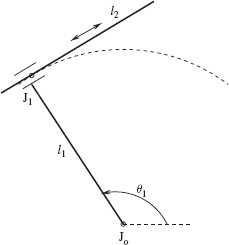

1The term “reactive planning” that is used sometimes in literature in reference to sensor-based motion planning is unfortunate: It emphasizes the operation's local nature, suggests that intelligence is not necessary, and hides the global component of motion planning, with its algorithmic connections to convergence and computational complexity.
2In other variations of this problem, one starts inside the maze and tries to find an exit from it; or, one starts outside the maze and tries to reach the location with a hidden treasure somewhere inside the labyrinth.
3A good survey of the work on provable algorithms for the Piano Mover's problem can be found in Ref. 11; specialized maze search algorithms are considered in Ref. 12.
4Higher dimensions d appear when one takes into account the moving rigid object's orientation along its way; d = 3 for the 2D case, and d = 6 for the 3D case.
5Less rigorous ways may include, for example, a direct comparison of an algorithm's results with those of other existing algorithms, or with the performance of an “average” human traveler.
6Eventually this question did appear in graph theory, though much later, as a question of existence of local algorithms [39].
7Interestingly, when in the 1960s and 1970s researchers turned to the problem of robot motion planning, the question of input information was not raised either. There seems to be something in human psychology that, unless told otherwise, between two choices—minimum and maximum of input information—we implicitly assume the latter.
8One name for procedures that combine localization and motion planning is SLAM, which stands for Simultaneous Localization and Motion Planning (see, e.g., Ref. 55).
9The procedure has been frequently suggested to me at various meetings.
Sensing, Intelligence, Motion, by Vladimir J. Lumelsky
Copyright © 2006 John Wiley & Sons, Inc.