 CHAPTER 7
Human Performance in Motion Planning
I … do not direct myself so badly. If it looks ugly on the right, I take the left … Have I left something unseen behind me? I go back; it is still on my road. I trace no fixed line, either straight or crooked.
—Michel de Montaigne (1533–1592), The Essays
7.1 INTRODUCTION
It is time to admit that we will not be able to completely fulfill the promise contained in this book's subtitle—explain how humans plan their motion. This would be good to do—such knowledge would help us in many areas—but we are not in a position to do so. Today we know precious little about how human motion decision-making works, certainly not on the level of algorithmic detail comparable to what we know about robot motion planning. To be sure, in the literature on psychophysical and cognitive science analysis of human motor skills one will find speculations about the nature of human motion planning strategies. One can even come up with experimental tests designed to elucidate such strategies. The fact is, however, that the sum of this knowledge tells us only what those human strategies might be, not what they are.
Whatever those unknown strategies that humans use to move around, we can, however, study those strategies' performance. By using special tests, adhering to carefully calibrated test protocols designed to elucidate the right questions, and by carrying out those tests on statistically significant groups of human subjects, we can resolve how good we humans are at planning our motion. Furthermore, we can (and will) subject robot sensor-based motion planning algorithms to the same tests—making sure we keep the same test conditions—and make far-reaching conclusions that can be used in the design of complex systems involving human operators.
Clearly, the process of testing human subjects has to be very different from the process of designing and testing robot algorithms that we undertook in prior chapters. This dictates a dramatic change in language and methodology. So far, as we dealt with algorithms, concepts have been specific and well-defined, statements have been proven, and algorithms were designed based on robust analysis. We had definitions, lemmas, theorems, and formal algorithms. We talked about algorithm convergence and about numerical bounds on the algorithm performance.
All such concepts become elusive when one turns to studying human motion planning. This is not a fault of ours but the essence of the topic. One way to compensate for the fuzziness is the black box approach, which is often used in physics, cybernetics, and artificial intelligence: The observer administers to the object of study—here a human subject—a test with a well-controlled input, observes the results at the output, and attempts to uncover the law (or the algorithm) that transfers one into the other.
With an object as complex as a human being, it would not be realistic to expect from this approach a precise description of motion planning strategies that humans use. What we expect instead from such experiments is a measure of human performance, of human skills in motion planning. By using techniques common in cognitive sciences and psychology, we should be able to arrive at crisp comparisons and solid conclusions. Why do we want to do this? What are the expected scientific and practical uses of this study?
One use is in the design of teleoperated systems—that is, systems with remotely controlled moving machinery and with a human operator being a part of the control and decision-making loop. In this interesting domain the issues of human and robot performance intersect. More often than not, such systems are very complex, very expensive, and very important. Typical examples include control of the arm manipulator at the Space Shuttle, control of arms at the International Space Station, and robot systems used for repair and maintenance in nuclear reactors.
The common view on the subject is that in order to efficiently integrate the human operator into the teleoperated system's decision-making and control, the following two components are needed: (1) a data gathering and preprocessing system that provides the operator with qualitatively and quantitatively adequate input information; this can be done using fixed or moving TV cameras and monitors looking at the scene from different directions, and possibly other sensors; and (2) a high-quality master–slave system that allows the operator to easily enter control commands and to efficiently translate them into the slave manipulator (which is the actual robot) motion.
Consequently, designers of teleoperation systems concentrate on issues immediately related to these two components (see, e.g., Refs. 116–119). The implicit assumption in such focus on technology is that one component that can be fully trusted is the human operator: As long as the right hardware is there, the operator is believed to deliver the expected results. It is only when one closely observes the operation of some such highly sophisticated and accurate systems that one perceives their low overall efficiency and the awkwardness of interactions between the operator and the system. One is left with the feeling that while the two components above are necessary, they are far from being sufficient.
Even in simple teleoperation tasks that would be trivial for a human child, like building a tower out of a few toy blocks or executing a collision-free motion between a few obstacles, the result is far from perfect: Unwanted collisions do occur, and the robot arm's motion is far from confident. The operator will likely move the arm maddeningly slowly and tentatively, stopping often to assess the situation. One becomes convinced that these difficulties are not merely a result of a (potentially improvable) inferior mechanical structure or control system, but are instead related to cognitive difficulties on the part of the operator. This is an exciting topic for a cognitive scientist, with important practical consequences.
To summarize, here are a few reasons for attempting a comparison between human and robot performance in motion planning:
- Algorithm Quality. Sensor-based motion planning algorithms developed in the preceding chapters leave a question unanswered: How good are they? If they produced optimal solutions, they would be easy to praise. But in a situation with limited input information the solutions are usually far from optimal, and assessing them is difficult. One way to assess those solutions is in comparison with human performance. After all, humans are used to solving motion planning problems under uncertainty and therefore must be a good benchmark.
- Improving Algorithms. If robot performance turns out to be inferior to human performance, this fact will provide a good incentive to try to understand which additional algorithmic resources could be brought to bear to improve robot motion planning strategies.
- Synergistic Teleoperation Systems. If, on the other hand, human performance can be inferior to robot performance—which we will observe to be so in some motion planning tasks—this will present a serious challenge for designers of practical teleoperation systems. It would then make sense to shift to robots some motion planning tasks that have been hitherto the sole responsibility of humans. We will observe that humans have difficulty guiding arm manipulators in a crowded space, resulting in mistakes or, more often, in a drastic reduction of the robot's speed to accommodate human “thinking.” Complementing human intelligence with appropriate robot intelligence may become a way of dramatically improving the performance of teleoperated systems.
- Cognitive Science. Human performance in motion planning is of much interest to cognitive scientists who study human motor skills and the interface between human sensory apparatus and motion. The performance comparison with robot algorithms in tasks that require motion planning might shed light on the nature of human cognitive processes related to motion in space.
To be meaningful, a comparison between human and robot performance must take place under exactly the same conditions. This is very important: It makes no sense, for example, to compare the performance of a human who moves around blindfolded with the performance of a robot that has a full use of its vision sensor. Other conditions may be more subtle: For instance, how do we make sure that in the same scene the robot and the human have access to exactly the same information? While one can never be absolutely sure that the conditions under which human and robot performance are compared are indeed equal, every effort has been made to ascertain this in our study.
To formulate the right questions, we will start in the next section with observations from a few experiments, and then move in the following sections to a consistent study with more representative tests and statistics. Most of those limited experiments have been done by the author in the late 1980s while at Yale University.1
The surprising, sometimes seemingly bizarre results from these experiments helped prompt discussion and sharpen our questions, but also indicated a need for a more consistent study. The larger, better designed, and much more consistent studies discussed in Sections 7.4 and 7.5 were undertaken in the mid-1990s at the University of Wisconsin—Madison, within a joint project between two groups: on the robotics side, by the author and graduate student Fei Liu, and on the cognitive science side, by Dr. Sheena Rogers and graduate student Jeffrey Watson, both from the University of Wisconsin Psychology Department's Center for Human Performance in Complex Systems.
7.2 PRELIMINARY OBSERVATIONS
We will start with a task that is relatively intuitive for a human—walking in a labyrinth (a maze)—and will then proceed to the less intuitive task of moving a simple planar two-link arm manipulator, of the kind that we considered in Section 5.2 (see Figures 5.2 and 5.15). It is important to realize that in some formal sense, both tasks are of the same difficulty: Moving in a maze amounts to controlling a combination of two variables, x and y (horizontal and vertical displacement), and moving a two-link arm also requires control of two variables, representing angular displacement (call these angles θ1 and θ2).
7.2.1 Moving in a Maze
Many of us have tried to walk in a labyrinth (a maze). Some medieval monasteries and churches have had labyrinths on the premises, or even indoors, to entertain its visitors. Today labyrinths appear in public and amusement parks. The labyrinth corridors are often made of live bushes cut neatly to make straight-line and curved walls. The wall may be low, to allow one to see the surrounding walls; in a more challenging labyrinth the walls are tall, so that at any given moment the walker can only see the surrounding walls. The visitor may start inside or outside of the labyrinth and attempt to reach the center, or locate a “treasure” inside the labyrinth, or find an exit from it.
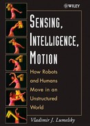
Moving with Complete Information. If one has a bird's-eye view of the whole labyrinth, this makes the task much easier. To study human performance in motion planning consistently, we start with this simpler task. Consider the bird's-eye view of a labyrinth shown in Figure 7.1. Imagine you are handed this picture and asked to produce in it a collision-free path from the position S (Start) to the target point T. One way to accomplish this test is with the help of computer. You sit in front of the computer screen, which shows the labyrinth, Figure 7.1. Starting at point S, you move the cursor on the screen using the computer mouse, trying to get to T while not banging into the labyrinth walls. At all times you see the labyrinth, points S and T, and your own position in the labyrinth as shown by the cursor. For future analysis, your whole path is stored in the computer's memory.
If you are a typical labyrinth explorer, you will likely study the labyrinth for 10–15 seconds, and think of a more or less complete path even before you start walking. Then you quickly execute the path on the screen. Your path will likely be something akin to the three examples shown in Figure 7.2. All examples demonstrate exemplary performance; in fact, these paths are close to the optimal—that is, the shortest—path from S to T.2 In the terminology used in this text, what you have done here and what the paths in Figure 7.2 demonstrate is motion planning with complete information.
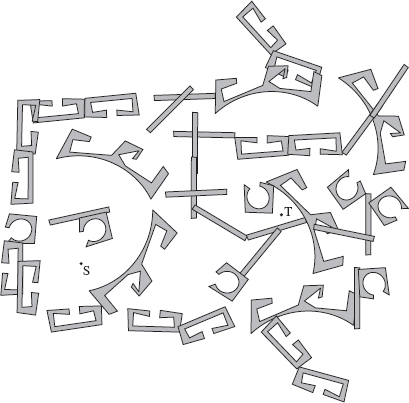
Figure 7.1 A two-dimensional labyrinth. The goal is to proceed from point S to point T.
If one tried to program a computer to do the same job, one would first preprocess the labyrinth to describe it formally—perhaps segment the labyrinth walls into small pieces, approximate those pieces by straight lines and polynomials for a more efficient description, and so on, and eventually feed this description into a special database. Then this information could be processed, for example, with one or another motion planning algorithm that deals with complete information about the task.
The level of detail and the respectable amount of information that this database would encompass suggests that this method differs significantly from the one you just used. It is safe to propose that you have paid no attention to small details when attempting your solution, and did not try to take into account the exact shapes and dimensions of every nook and cranny. More likely you concentrated on some general properties of the labyrinth, such as openings in walls and where those openings led and whether an opening led to a dead end. In other words, you limited your attention to the wall connectivity and ignored exact geometry, thus dramatically simplifying the problem. Someone observing you—call this person the tester—would likely conclude that you possess some powerful motion planning algorithm that you applied quickly and with no hesitation. Since it is very likely that you never had a crash course on labyrinth traversal, the source and nature of your powerful algorithm would present an interesting puzzle for the tester.
Today we have no motion planning algorithms that, given complete information about the scene, will know from the start which information can be safely ignored and that will solve the task with the effectiveness you have demonstrated a minute ago. The existing planning algorithms with complete information will grind through the whole database and come up with the solution, which is likely to be almost identical to the one you have produced using much less information about the scene. The common dogma that humans are smarter than computers is self-evident in this example.
Moving with Incomplete Information. What about a more realistic labyrinth walk, where at any given moment the walker can see only the surrounding walls? To test this case, let us use the same labyrinth that we used above (Figure 7.1), except that we modify the user interface to reflect the new situation. As before, you are sitting in front of the computer screen. You see on it only points S and T and your own position in the labyrinth (the cursor). The whole labyrinth is there, but it is invisible. As before, you start at S, moving the cursor with the computer mouse. Every time the cursor approaches a labyrinth wall within some small distance—that is your “radius of vision”—the part of the wall within this radius becomes visible, and so you can decide where to turn to continue the motion. Once you step back from the wall, that piece of the wall disappears from the screen.

Figure 7.2 Three paths produced by human subjects in the labyrinth of Figure 7.1, if given the complete information, the bird's-eye view of the scene.
Your performance in this new setting will of course deteriorate compared to the case with complete information above. You will likely wander around, hitting dead ends and passing some segments of the path more than once. Because you cannot now see the whole labyrinth, there will be no hope of producing a near-optimal solution; you will struggle just to get somehow to point T. This is demonstrated in two examples of tests with human subjects shown in Figure 7.3. Among the many such samples with human subjects that were obtained in the course of this study (see the following sections), these two are closest to the best and worst performance, respectively. Most subjects fell somewhere in between.
While this performance is far from what we saw in the test with complete information, it is nothing to be ashamed of—the test is far from trivial. Those who had a chance to participate in youth wilderness training know how hard one has to work to find a specific spot in the forest, with or without a map. And many of us know the frustration of looking for a specific room in a large unfamiliar building, in spite of its well-structured design.
Human Versus Computer Performance in a Labyrinth. How about comparing the human performance we just observed with the performance of a decent motion planning algorithm? The computer clearly wins. For example, the Bug2 algorithm developed in Section 3.3.2, operating under the same conditions as for the human subjects, in the version with incomplete information produces elegant solutions shown in Figure 7.4: In case (a) the “robot” uses tactile information, and in case (b) it uses vision, with a limited radius of vision rυ, as shown.
Notice the remarkable performance of the algorithm in Figure 7.4b: The path produced by algorithm Bug2, using very limited input information—in fact, a fraction of complete information—almost matches the nearly optimal solution in Figure 7.2a that was obtained with complete information.
We can only speculate about the nature of the inferior performance of humans in motion planning with incomplete information. The examples above suggest that humans tend to be inconsistent (one might say, lacking discipline): Some new idea catches the eye of the subject, and he or she proceeds to try it, without thinking much about what this change will mean for the overall outcome.
The good news is that it is quite easy to teach human subjects how to use a good algorithm, and hence acquire consistency and discipline. With a little practice with the Bug2 algorithm, for example, the subjects started producing paths very similar to those shown in Figure 7.4.
This last point—that humans can easily master motion planning algorithms for moving in a labyrinth—is particularly important. As we will see in the next section, the situation changes dramatically when human subjects attempt motion planning for arm manipulators. We will want to return to this comparison when discussing the corresponding tests, so let us repeat the conclusion from the above discussion:

Figure 7.3 Two examples of human performance when operating in the labyrinth of Figure 7.1 with incomplete information about the scene. Sample (a) is closer to the best performance, while sample (b) is closer to the worst performance observed in this study.
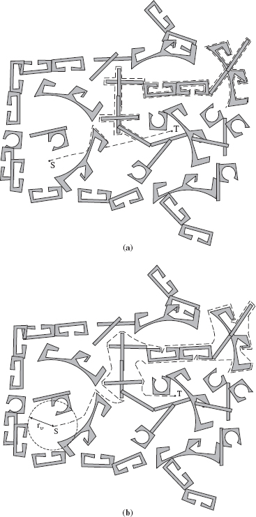
Figure 7.4 Performance of algorithm Bug2 (Chapter 3) in the labyrinth of Figure 7.1. (a) With tactile sensing and (b) with vision that is limited to radius rυ.
When operating in a labyrinth, humans have no difficulty learning and using motion planning algorithms with incomplete information.
7.2.2 Moving an Arm Manipulator
Operating with Complete Information. We are now approaching the main point of this discussion. There was nothing surprising about the human performance in a labyrinth; by and large, the examples of maze exploration above agree with our intuition. We expected that humans would be good at moving in a labyrinth when seeing all of it (moving with complete information), not so good when moving in a labyrinth “in the dark” (moving with incomplete information), and quite good at mastering a motion planning algorithm, and this is what happened. We can use these examples as a kind of a benchmark for assessing human performance in motion planning.
We now turn to testing human performance in moving a simple two-link revolute-revolute arm, shown in Figure 7.5. As before, the subject is sitting in front of the computer screen, and controls the arm motion using the computer mouse. The first link, l1, of the arm rotates about its joint J0 located at the fixed base of the arm. The joint of the second link, J1, is attached to the first link, and the link rotates about point J1, which moves together with link l1. Overall, the arm looks like a human arm, except that the second link, l2, has a piece that extends outside the “elbow” J1. (This kinematics is quite common in industrial and other manipulators.) And, of course, the arm moves only in the plane of the screen.

Figure 7.5 This simple planar two-link revolute-revolute arm manipulator was used to test human performance in motion planning for a kinematic structure: l1 and l2 are two links; J0 and J1 are two revolute joints; θ1 and θ2 are joint angles; S and T are start and target positions in the test; P is the arm endpoint in its current position; O1, O2, O3, and O4 are obstacles.
How does one control the arm motion in this setup? By positioning the cursor on link l1 and holding down the mouse button, the subject will make the link rotate about joint J0 and follow the cursor. At this time link l2 will be “frozen” relative to link l1 and hence move with it. Similarly, positioning the cursor on link l2 and holding down the mouse button will make the second link rotate about joint J1, with link l1 being “frozen” (and hence not moving at all). Each such motion causes the appropriate link endpoint to rotate on a circular arc.
Or—this is another way to control the arm motion—one can position the cursor at the endpoint P of link l2 and drag it to whatever position in the arm workspace one desires, instantaneously or in a smooth motion. The arm endpoint will follow the cursor motion, with both links moving accordingly. During this motion the corresponding positions of both links are computed automatically in real time, using the inverse kinematics equations. (Subjects are not told about this mechanism, they just see that the arm moves as they expect.) This second option allows one to control both links motion simultaneously. It is as if someone moves your hand on the table—your arm will follow the motion.
We will assume that, unlike in the human arm, there are no limits to the motion of each joint in Figure 7.5. That is, each link can in principle rotate clockwise or counterclockwise indefinitely. Of course, after every 2π each link returns to its initial position, so one may or may not want to use this capability. [Looking ahead, sometimes this property comes in handy. When struggling with moving around an obstacle, a subject may produce more than one rotation of a link. Whether or not the same motion could be done without the more-than-2π link rotation, not having to deal with a constraint on joint angle limits makes the test psychologically easier for the subject.]
The difficulty of the test is, of course, that the arm workspace contains obstacles. When attempting to move the arm to a specified target position, the subjects will need to maneuver around those obstacles. In Figure 7.5 there are four obstacles. One can safely guess, for example, that obstacle O1 may interfere with the motion of link l1 and that the other three obstacles may interfere with the motion of link l2.
Similar to the test with a labyrinth, in the arm manipulator test with complete information the subject is given the equivalent of the bird's-eye view: One has a complete view of the arm and the obstacles, as shown in Figure 7.5. Imagine you are that subject. You are asked to move the arm, collision-free, from its starting position S to the target position T. The arm may touch an obstacle, but the system will not let you move the arm “through” an obstacle. Take your time—time is not a consideration in this test.
Three examples of performance by human subjects in controlled experiments are shown in Figure 7.6.3 Shown are the arm's starting and target positions S and T, along with the trajectory (dotted line) of the arm endpoint on its way from S to T. The examples represent what one might call an “average” performance by human subjects.4
The reader will likely be surprised by these samples. Why is human performance so unimpressive? After all, the subjects had complete information about the scene, and the problem was formally of the same (rather low) complexity as in the labyrinth test. The difference between the two sets of tests is indeed dramatic: Under similar conditions the human subjects produced almost optimal paths in the labyrinth (Figure 7.2) but produced rather mediocre results in the test with the arm (Figure 7.6).
Why, in spite of seeing the whole scene with the arm and obstacles (Figure 7.5), the subjects exhibited such low skills and such little understanding of the task. Is there perhaps something wrong with the test protocol, or with control means of the human interface—or is it indeed real human skills that are represented here? Would the subjects improve with practice? Given enough time, would they perhaps be able to work out a consistent strategy? Can they learn an existing algorithm if offered this opportunity? Finally, subjects themselves might comment that whereas the arm's work space seemed relatively uncluttered with obstacles, in the test they had a sense that the space was very crowded and “left no room for maneuvering.”
The situation becomes clearer in the arm's configuration space (C-space, Figure 7.7). As explained in Section 5.2.1, the C-space of this revolute–revolute arm is a common torus (see Figure 5.5). Figure 7.7 is obtained by flattening the torus by cutting it at point T along the axes θ1 and θ2. This produces four points T in the resulting square, all identified, and two pairs of identified C-space boundaries, each pair corresponding to the opposite sides of the C-space square. For reference, four “shortest” paths (M-lines) between points S and T are shown (they also appear in Figure 5.5; see the discussion on this in Section 5.2.1). The dark areas in Figure 7.7 are C-space obstacles that correspond to the four obstacles in Figure 7.5.
Note that the C-space is quite crowded, much more than one would think when looking at Figure 7.5. By mentally following in Figure 7.7 obstacle outlines across the C-space square boundaries, one will note that all four workspace obstacles actually form a single obstacle in C-space. This simply means that when touching one obstacle in work space, the arm may also touch some other obstacle, and this is true sequentially, for pairs (O1, O2), (O2, O3), (O3, O4), (O4, O1). No wonder the subjects found the task difficult. In real-world tasks, such interaction happens all the time; and the difficulties only increase with more complex multilink arms and in three-dimensional space.
Figure 7.6 Paths produced by three human subjects with the arm shown in Figure 7.5, given complete information about the scene.

Figure 7.7 C-space of the arm and obstacles shown in Figure 7.5.
Operating the Arm with Incomplete Information. Similar to the test with incomplete information in the labyrinth, here a subject would at all times see points S and T, along with the arm in its current positions. Obstacles would be hidden. Thus the subject moves the arm “in the dark”: When during its motion the arm comes in contact with an obstacle—or, in the second version of the test, some parts of the obstacle come within a given “radius of vision” rυ from some arm's points—those obstacle parts become temporarily visible. Once the contact is lost—or, in the second version, once the arm-to-obstacle distance increases beyond rυ—the obstacle is again invisible.
The puzzling observation in such tests is that, unlike in the tests with the labyrinth, the subjects' performance in moving the arm “in the dark” is on average indistinguishable from the test with complete information. In fact, some subjects performed better when operating with complete information, while others performed better when operating “in the dark.” One subject did quite well “in the dark,” then was not even able to finish the task when operating with a completely visible scene, and refused to accept that in both cases he had dealt with the same scene: “This one [with complete information] is much harder; I think it has no solution.” It seems that extra information doesn't help. What's going on?
Human Versus Computer Performance with the Arm. As we did above with the labyrinth, we can attempt a comparison between the human and computer performance when moving the arm manipulator, under the same conditions. Since in previous examples human performance was similar in tests with complete and incomplete information, it is not important which to consider: For example, the performance shown in Figure 7.6 is representative enough for our informal comparison. On the algorithm side, however, the input information factor makes a tremendous difference—as it should. The comparison becomes interesting when the computer algorithm operates with incomplete (“sensing”) information.
Shown in Figure 7.8 is the path generated in the same work space of Figure 7.5 by the motion planning algorithm developed in Section 5.2.2. The algorithm operates under the model with incomplete information. To repeat, its sole input information comes from the arm sensing; known at all times are only the arm positions S and T and its current position. The arm's sensing is assumed to allow the arm to sense surrounding objects at every point of its body, within some modest distance rυ from that point. In Figure 7.8, radius rυ is equal to about half of the link l1 thickness; such sensing is readily achievable today in practice (see Chapter 8).

Figure 7.8 Path produced in the work space of Figure 7.5 by the motion planning algorithm from Section 5.2.2; M1 is the shortest (in C-space) path that would be produced if there were no obstacles in the workspace.
Similar to Figure 7.6, the resulting path in Figure 7.8 (dotted line) is the path traversed by the arm endpoint when moving from position S to position T. Recall that the algorithm takes as its base path (called M-line) one of the four possible “shortest” straight lines in the arm's C-space (see lines M1, M2, M3, M4 in Figure 5.5); distances and path lengths are measured in C-space in radians. In the example in Figure 7.8, the shortest of these four is chosen (it is shown as line M1, a dashed line). In other words, if no obstacles were present, under the algorithm the arm endpoint would have moved along the curve M1; given the obstacles, it went along the dotted line path.
The elegant algorithm-generated path in Figure 7.8 is not only shorter than those generated by human subjects (Figure 7.6). Notice the dramatic difference between the corresponding (human versus computer) arm test and the labyrinth test. While a path produced in the labyrinth by the computer algorithm (Figure 7.4) presents no conceptual difficulty for an average human subject, they find the path in Figure 7.8 incomprehensible. What is the logic behind those sweeping curves? Is this a good way to move the arm from S to T? The best way? Consequently, while human subjects can easily master the algorithm in the labyrinth case, they find it hard—in fact, seemingly impossible—to make use of the algorithm for the arm manipulator.
7.2.3 Conclusions and Plan for Experiment Design
We will now summarize the observations made in the previous section, and will pose a few questions that will help us design a more comprehensive study of human cognitive skills in space reasoning and motion planning:
- The labyrinth test is a good easy-case benchmark for testing one's general space reasoning abilities, and it should be included in the battery of tests. There are a few reasons for this: (a) If a person finds it difficult to move in the labyrinth—which happens rarely—he or she will be unlikely to handle the arm manipulator test. (b) The labyrinth test prepares a subject for the test with an easier task, making the switch to the arm test more gradual. (c) A subject's successful operation in the labyrinth test suggests that whatever difficulty the subject may have with the arm test, it likely relates to the subject's cognitive difficulties rather than to the test design or test protocol.
- When moving the arm, subjects exhibit different tastes for control means: Some subjects, for example, prefer to change both joint angles simultaneously, “pulling” the arm endpoint in the direction they desire, whereas other subjects prefer to move one joint at the time, thus producing circular arcs in the path; see Figure 7.6. Because neither technique seems inherently better or easier than the other, for subjects' convenience both types of control should be available to them during the test.
- Since working with a bird's-eye view (complete information) as opposed to “in the dark” (incomplete information) makes a difference—clearly so in the labyrinth test and seemingly less so in the arm manipulator test—this dichotomy should be consistently checked out in the comprehensive study.
- In the arm manipulator test it has been observed that the direction of arm motion may have a consistent effect on the subjects' performance. Obviously, in the labyrinth test this effect appears only when operating with incomplete information (“moving in the dark”). This effect is, however, quite pronounced in either test with the arm manipulator, with complete or with incomplete information. Namely, in the setting of Figure 7.5, the generated path and the time to finish were noted to be consistently longer when moving from position T to S than when moving from S to T. This suggests that it is worthwhile to include the direction of motion as a factor in the overall test battery. (And, the test protocol should be set up so that the order of subtests has no effect on the test results.) One possible reason for this peculiar phenomenon is a psychological effect of one's paying more attention to route alternatives that are closer to the direction of the intended route than to those in other directions. Consider the simple “labyrinth” shown in Figure 7.9: The task is to reach one point (S or T) from the other while moving “in the dark.” When walking from S to T, most subjects will be less inclined to explore the dead-end corridor A because it leads in a direction almost opposite to the direction toward T, and they will on average produce shorter paths. On the other hand, when walking from T to S, more subjects will perceive corridor A as a promising direction and will, on average, produce longer paths. Such considerations are harder to pinpoint for the arm test, but they do seem to play a role.5
- The less-than-ideal performance of the subjects in the arm manipulator tests makes one wonder if something else is at work here. Can it be that the human-computer interface offered to the subjects is somewhat “unnatural” for them—and this fact, rather than their cognitive abilities, is to blame for their poor performance? Some subjects did indeed blame the computer interface for their poor performance.6 Some subjects believed that their performance would improve dramatically if they had a chance to operate a physical arm rather than a virtual arm on the computer screen (“if I had a real thing to grab and move in physical space, I would do much better…”). This is a serious argument; it suggests that adding a physical test to the overall test battery might provide interesting results.
Figure 7.9 In this simplistic maze, the subjects seem less inclined to explore the dead-end corridor A when walking from S to T than when walking from T to S.
- Based on standard practice for cognitive tests, along with some subjects' comments, it is worthwhile to explore human motion planning skills along some demographic lines. For example,
- Performance as a function of gender (consider the proverbial proficiency of men in handling maps).
- Performance as a function of age: For example, are children better than adults in spatial reasoning tasks (as they seem to be in some computer games or with the Rubik's Cube)?
- Performance as a function of educational level and professional orientation: For example, wouldn't we expect students majoring in mechanical engineering to do better in our tests than students majoring in comparative literature?
- Finally, there is an important question of training and practice. We all know that with proper training, people achieve miracles in motion planning; just think of an acrobat on a high trapeze. In the examples above, subjects were given a chance to get used to the task before a formal test was carried out, but no attempt was made to consistently study the effect of practice on human performance. The effect of training is especially serious in the case of arm operation, in view of the growing area of teleoperation tasks (consider the arm operator on the Space Shuttle, or a partially disabled person commanding an arm manipulator to take food from the refrigerator). This suggests that the training factor must be a part of the larger study.

This list covers a good number of issues and consequently calls for a rather ambitious study. In the specific study described below, not all questions on the list have been addressed thoroughly enough, due to the difficulty of arranging a statistically representative group of subjects. Some questions were addressed only cursorily. For example, attempts to enlist in the experiment a local kindergarten or a primary school had a limited success, and so was an attempt to round up enough subjects over the age of 60.
The very limited number of tests carried out for these insufficiently studied issues provide these observations: (a) Children do not seem to do better than adults in our tests. (b) Subjects aged 60 and over seem to have significantly more difficulty carrying out the tests: in the arm test, in particular, they would give up more often than younger subjects before reaching the solution. (c) The level of one's education and professional orientation seems to play an insignificant role: Secretaries do as well or as poorly as mechanical engineering PhDs or professional pilots, who pride themselves in their spatial reasoning.
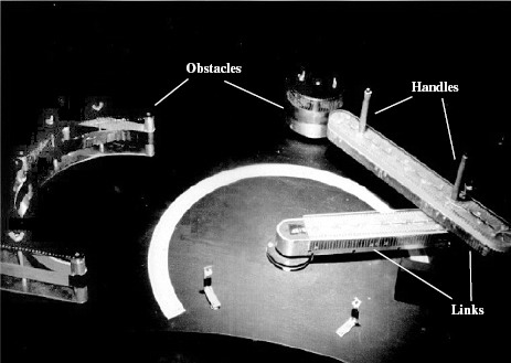
Figure 7.10 The physical two-link arm used in the tests of human performance.
The Physical Arm Test Setup. This experimental system has been set up in a special booth, with about 5 ft by 5 ft floor area, enough to accommodate a table with the two-link arm and obstacles, and a standing subject. The inside of the booth is painted black, to help with the “move in the dark” test. For a valid comparison of subjects' performance with the virtual environment test, the physical arm and obstacles (Figure 7.10) are proportionally similar to those in Figure 7.5. (Only two obstacles can be clearly seen in Figure 7.10; obstacle O1 of Figure 7.5 was replaced for technical reasons by two stops; see Figure 7.10.)
For the subjects' convenience the arm is positioned on a slightly slanted table. Each arm link is about 2 ft long. A subject moves one or both arm links using the handles shown. During the test the arm positions are sampled by potentiometers mounted on the joint axes, and they are documented in the host computer for further analysis, together with the corresponding timing information.7
Special features have been added for testing the scene visibility factor. Opening the booth doors and turning on its light produces the visible scene; closing the door shut and turning off the light makes it an invisible environment. For the latter test, the side surfaces of the arm links and of the obstacles are equipped with densely spaced contacts and LED elements located along perimeters of both links (Figure 7.10). There are 117 such LEDs on the inner link (link 1) and 173 LEDs on the outer link (link 2). When a link touches an obstacle, one or more LEDs light up, informing the subject of a collision and giving its exact location. Visually, the effect is similar to how a contact is shown in the virtual arm test.8
7.3 EXPERIMENT DESIGN
7.3.1 The Setup
Two batteries of tests, called Experiment One and Experiment Two, have been carried out to address the issues listed in the previous section. Experiment One addresses the effect of three factors on human performance: interface factor, which focuses on the effect of a virtual versus physical interface; visibility factor, which relates to the subject's seeing the whole scene versus the subject's “moving in the dark”; and direction factor, which deals with the effect of the direction of motion in the same scene. Each factor is therefore a dichotomy with two levels. We are especially interested in the effects of interface and visibility, since these affect most directly one's performance in motion planning tasks. The direction of motion is a secondary factor, added to help clarify the effect of the other two factors.
Experiment Two is devoted specifically to the effect of training on one's performance. The effect is studied in the context of the factors described above. One additional factor here, serving an auxiliary role, is the object-to-move factor, which distinguishes between moving a point robot in a labyrinth versus moving a two-link arm manipulator among obstacles. The arm test is the primary focus of this study; the labyrinth test is used only as a benchmark, to introduce the human subjects to the tests' objectives.
The complete list of factors, each with two levels (settings), is therefore as follows9:
- Object-to-move factor, with two levels:
- Moving a point robot in a labyrinth, as in Figure 7.1.
- Moving a two-link revolute-revolute arm manipulator in a planar workspace with obstacles, as in Figure 7.5.
- Interface factor, with two levels:
- In this test, called the virtual test, the subject operates on the computer screen, moving the arm links with the computer mouse; all necessary help is done by the underlying software. Both the labyrinth test (Figure 7.1) and the arm test (Figure 7.5) are done in this version.
- In this test, called the physical test, the subject works in the booth, moving the physical arm (Figure 7.10). Only the arm tests, and no labyrinth tests, were done in this version.
- Visibility factor, with two levels:
- Visible environment: The object (one of those in factor A) and its environment are fully visible.
- Invisible environment: Obstacles cannot be seen by the subject, except when the robot (in case of the point robot) or a part of its body (in case of the arm) is close enough to an obstacle, in which case a small part of the obstacle near the contact point becomes visible for the duration of contact. The arm is visible at all times.
- Direction factor (for the arm manipulator test only), with two levels:
- “Left-to-right” motion (denoted below LtoR), as in Figure 7.8.
- “Right-to-left” motion (denoted RtoL); in Figure 7.8 this would correspond to moving the arm from position T to position S.
- Training factor. The goal here is to study the effect of prior learning and practice on human performance. This factor is studied in combination with all prior factors and has two levels:
- Subjects' performance with no prior training. Here the subjects are only explained the rules and controls, and are given the opportunity to try and get comfortable with the setup, before the actual test starts.
- Subjects' performance is measured after a substantial prior training and practice.
Therefore, the focus of Experiment One is on factors B, C, and D, and the focus of Experiment Two is on factor E (with the tests based on the same factors B, C, and D). Because each factor is a dichotomy with two levels, all possible combinations of levels for factors B, C, and D produce eight tasks that each subject can be subjected to:
- Task 1: Virtual, visible, left-to-right
- Task 2: Virtual, visible, right-to-left
- Task 3: Virtual, invisible, left-to-right
- Task 4: Virtual, invisible, right-to-left
- Task 5: Physical, visible, left-to-right
- Task 6: Physical, visible, right-to-left
- Task 7: Physical, invisible, left-to-right
- Task 8: Physical, invisible, right-to-left
In addition to these tasks, a smaller study was carried out to measure the effect of three auxiliary variables:
(a) gender, with values “males” and “females”,
(b) specialization, with values “engineering,” “natural sciences,” and “social sciences”, and
(c) age, with values “15–24,” “25–34”, and “above 34”.
A total of 48 subjects have been tested in Experiment One, with the following distribution between genders, specializations, and age groups:
- Gender: 23 males and 25 females
- Specialization: engineering, 16; natural sciences, 20; social sciences, 12
- Age groups: age 15–24, 32 subjects; age 25–34, 12 subjects; age above 34, 4 subjects
From the standpoint of statistical tests, subjects have been selected randomly, and so test observations can be considered mutually independent.
One problem that must be addressed in the test protocol is avoiding the learning effect: We need to prevent the subjects from using in one test the knowledge that they acquired in a prior test. Then one's performance is independent of the order of tasks execution. This is important when randomly varying the order of tasks between subjects, a standard technique in cognitive skills tests. This has been achieved by making each subject go through 4 out of 8 tasks. For example, a subject who went through the virtual–visible–LtoR task would not be subjected to the virtual–visible–RtoL task. With this constraint, half of the subject pool did tasks 1, 4, 5, 8, while the other half did tasks 2, 3, 6, and 7 from the list above.
As a result, each of the eight tasks should have 24 related observation sets, each set including the path length, the completion time, and the actual data on the generated path for one subject. (In reality, two observation sets for the physical test, one for the visible–RtoL and the other for the invisible-LtoR combination, were documented incorrectly and were subsequently discarded, leaving 23 observations for Task 6 and Task 7 each.)
Another way to group the observed data is by the three factors (interface, visibility, direction), each with two levels: (virtual, physical), (visible, invisible), and (LtoR, RtoL). This grouping produces six data sets and is useful for studying separate effects on human performance—for example, the effect on one's performance of moving a visible arm or moving left to right (see the next section). With two lost observations mentioned above, the sizes of the six data sets are as follows:
- Set 1: Interface data for “virtual”—96 observations
- Set 2: Interface data for “physical”—94 observations
- Set 3: Visibility data for “visible”—95 observations,
- Set 4: Visibility data for “invisible”—95 observations,
- Set 5: Direction data for “left to right”—95 observations,
- Set 6: Direction data for “right to left”—95 observations.
A total of 12 subjects have been tested in Experiment Two.
Performance Criteria. Two criteria have been used to measure subjects' performance in the tasks:
- The length of generated path (called Path)
- The task completion time (called Time)
In the labyrinth tests the path length is the actual length of the path a subject generates in the labyrinth. In the arm manipulator test the path length is measured as the sum of two modulo link rotation angles in radians. Time, in seconds, is the time it takes a subject to complete the task.
Statistical Considerations. In statistical terms, the length of path and the completion time are dependent variables, and the test conditions, as represented by factors and levels, are independent variables. If, for example, we want to compare the effect of a visible scene versus invisible scene on the length of paths produced by the subjects, then visibility is an independent variable (with two values, visible and invisible), and the length of path is a dependent variable.
As one would expect, the dependent variables Path and Time are highly correlated: In Experiment One the correlation coefficient between the two is r(Path, Time) = 0.74.
A multivariate observation for a particular subject is the set of scores of this subject in a given task; it is thus a vector. For example, for Subject 1 the dependent variable vector (Path, Time) in Task 1 (virtual-visible-LtoR) happened to be (59; 175).
The concept of statistical significance (see e.g., [127]) is a quantitative index of reliability of a given result or statement, usually in terms of a variable in question. Specifically, the significance p-level represents the probability of an error involved in accepting an observed result (or statement) as valid, or as representative of the population. In practice, results corresponding to the significance level p ≤ 0.05 are usually considered significant.
Put differently, p-level indicates the probability of error when rejecting some related null hypothesis. A null hypothesis, denoted as H0, relates to making a statement about the observation data—for example, when deciding whether two sets of data came from the same population of data. If a statistical test suggests that the null hypothesis should be rejected, say with significance level p ≤ 0.01, we can conclude that the two samples differ significantly, or that the variable of interest has a significant effect on the sample data. If the test results suggest accepting the null hypothesis, we conclude that the two samples do not differ significantly, and hence the variable of interest has no effect on the sample data.
7.3.2 Test Protocol
The salient characteristics of the test protocol can be summarized as follows (more details on the experiment design and test conditions can be found in Ref. 121):
- The primary focus in the study is on tests with the arm manipulator (see Figure 7.5). The labyrinth test is used only as a benchmark, for introducing the subjects to the tests and the study's underlying ideas.
- The bulk of the subject pool for this study was paid undergraduate students and also some graduate students. (There was no statistical difference in performance between the two groups.)
- In the first session, about one hour long, a subject would be taught how to carry out a test and would be given a pilot test to ascertain that he/she can be submitted to the test; the latter would be different from the pilot test.
- The maximum time a subject was given to finish the test with the arm manipulator was 15 minutes. Much less was allowed for the labyrinth test: As a rule, 1–2 minutes were enough. These limits were chosen as a rough estimate of the time the subjects would need to complete a test without feeling time pressure. Most subjects finished their tasks well within the time allocation; those few who didn't were not likely to finish even with significantly more time.
- Measures were taken to eliminate the effect of a subject's memory recall, or information passing, from one task to another. In the invisible version of the arm test, rotating the whole scene on the computer screen for a consequent session would practically eliminate the effect of memorization from prior sessions. This also helps from the test protocol standpoint: Using the same scene in subsequent tests allows for an “apples-with-apples” assessment of subjects' performance.
7.4 RESULTS–EXPERIMENT ONE
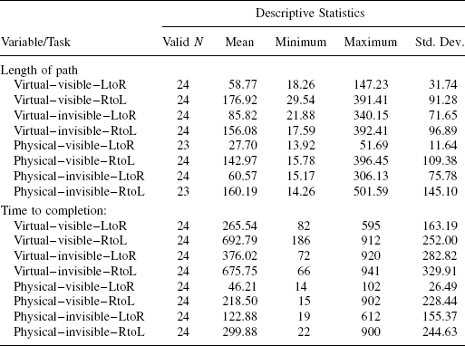
The basic (descriptive) statistics for motion planning tests carried out in Experiment One are given in Table 7.1. Statistics are given separately for each dependent variable, the length of path (Path) and the time to completion in seconds (Time), and within each dependent variable for each of the eight tasks listed in Section 7.3.1. Each line in Table 7.1 refers to a given task and includes the number of tested subjects (“Valid N” statistics) as well as the mean, minimum, maximum, and standard deviation of the correspondent variable.
A quick glance at the table provides a few observations that we will address in more detail later. One surprise is that the subjects' performance with the right-to-left direction of motion was significantly worse than their performance with the left-to-right direction of motion: Depending on the task, the mean length of path for the right-to-left direction is about two to five times longer than that for the left-to-right direction.10
Another surprise is that the statistics undermines the predominant belief among subjects and among robotics and cognitive science experts that humans should be doing significantly better when moving a physical as opposed to a virtual arm. Isn't the physical arm quite similar to our own arm, which we use so efficiently? To be sure, the subjects did better with the physical arm—but only a little better, not by as much as one would expect, and only for the (easier) left-to-right direction of motion. Once the task became a bit harder, the difference disappeared: When moving the physical arm in the right-to-left direction, more often than not the subjects' performance was significantly worse than when moving the virtual arm in the left-to-right direction, and more or less comparable to moving the virtual arm in the same right-to-left direction (see Table 7.1).
In other words, letting a subject move the physical arm does not guarantee more confidence than when moving a virtual arm: Some other factors seem to play a more decisive role in the subjects' performance. In an attempt to extract the (possibly hidden) effects of our experimental factors on one's performance, two types of analysis have been undertaken for the Experiment One data:
- The first one, Principal Components Analysis (PCA), has been carried out as a preliminary study, to understand the general nature of obtained observation data and to see if such factors as subjects' gender, specialization, and age group have a noticeable effect on the subjects' performance in motion planning tasks.
TABLE 7.1. Descriptive Statistics for the Data in Experiment One
- The second, more pointed analysis addresses separate effects of individual factors on subjects' performance—the effect of interface (virtual versus physical), scene visibility, and the direction of motion. This study makes use of tools of nonparametric analysis and univariate analysis of variance. Only brief summaries of the techniques used are presented below. For more details on the techniques the reader should refer to the sources cited in the text below; for details related to this specific study see Ref. 121.
7.4.1 Principal Components Analysis
We attempt to answer the following questions:
- To what extent are the factors used—interface (virtual or physical), scene visibility, and direction of motion—indicative of human performance?
- Can these factors be replaced by some “hidden” factors that describe the same data in a clearer and more compact way?
- Which factor or which part of the factor's variance is most indicative of one's performance in a motion planning task?
- Do the patterns of subjects' performance differ as a function of their gender, college specialization, and age group?
- Can we predict one's performance in one task based on their performance in another task?
Principal Components Analysis (PCA) addresses these questions based on analysis of the covariance matrix of the original set of independent variables [122, 123]. In our case this would be the covariance matrix of a set of two-level tasks. The analysis seeks to identify “hidden” factors—called the principal components—which turn out to be eigenvectors of the sample covariance matrix. The matrix's eigenvalues represent variation of the principal components; the sum of eigenvalues is the total variance of the original sample data and is equal to the sum of variances of the original variables.
With the principal components (eigenvectors) conveniently ordered from the largest to the smallest, the first component accounts for most of the total variance in the sample data, the second component accounts for the next biggest part of the total variance, and so on. The first component can thus be called the “most important hidden factor,” and so on. This ordering sometimes allows the researcher to (a) drop the last few components if they account for too small a part of the total variance and (b) claim that the data can be adequately described via a smaller set of variables. Often attempts are made to interpret the “hidden factors” in physical terms, arguing that if the hidden factors could be measured directly they would allow a significantly better description of the phenomenon under discussion.
Let X be the column matrix of the original sample data; its element xij is the value of the jth sample variable (the jth column vector of X) for the ith observation row vector (the ith subject, ith row of X). Denote the covariance matrix computed from the sample matrix X by R. Let matrix A contain as its column vectors the eigenvectors of matrix R: The ith column of A is the ith principal component of R. Both R and A are square matrices of the same rank (normally equal to the number of sample variables). Matrix A can then be seen as a transformation matrix that relates the original data to the principal components: Each original data point (described by a row vector of X) can now be described in terms of new coordinates (principal components), as a row vector z; hence
Let matrix ∧ be a diagonal matrix of the same rank, with eigenvalues of R in its diagonal positions, ordered from largest to smallest.
The matrix of principal component loadings, denoted by L, is
An element lij of the square matrix L is the correlation coefficient between the ith variable and the jth principal component. It informs us about the “importance,” or “contribution,” of the ith variable to the jth principal component. Geometrically, the loading is the projection of ith variable onto the jth component.
If only independent variables represented by the interface and visibility factors are considered in our arm test, this will include four out of the eight tasks listed in Section 7.3.1:
- virtual–visible
- virtual–invisible
- physical–visible
- physical–invisible
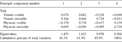
The loading matrix of the corresponding four principal components in the arm test is shown in Table 7.2. As seen in the table, the first PC (principal component) accounts for 36.3% of the total variance (top four numbers in column 1) and is tied primarily to the virtual–visible and physical–invisible tasks (0.679 and 0.695 loads, accordingly). The second PC accounts for the next 25.6% of the total variance and is tied primarily to the other two tasks, virtual-invisible and physical–visible (loads 0.666 and 0.739), and so on. Since the contribution of successive PCs into the total variance falls off rather smoothly, with 85.9% of the variance being accounted for by the first three PCs, we conclude (somewhat vaguely) that to a large extent the four tasks measure something different, each one bringing new information about the subjects' performance, and hence cannot be replaced by a smaller number of “hidden factors.”
TABLE 7.2. Loadings for the Principal Components in the Arm Manipulator Test
Using Eq. (7.1), the scores on all PCs can now be calculated for all subjects and plotted accordingly. The scores have been obtained and plotted in this study in various forms—for example, in three-dimensional space of the first three PCs and in two-dimensional plots for different pairs of PCs (e.g., a plot in plane PC1 versus PC2, etc.). By labeling the subjects (which become points in such plots) with additional information categories, such as their specialization majors, gender, and age, score plots regarding those categories have been also obtained.
These plots (see Ref. [121]) happen to provide no interesting conclusions about the importance of principal components or of their correlations with the subjects' specialization, gender, or age. Namely, we conclude that contrary to the common wisdom, engineering and computer science students, whose specialities can be expected to give them an edge in handling spatial reasoning tasks, have done no better than students with majors in the arts and social sciences. Also, men did no better than women.
This does not give us a right, however, to make sweeping conclusions of one sort or another. The Principal Component Analysis (PCA) is designed to study the input variables as a pack, and in particular to uncover the biggest sources of variation between independent variables of the original test data. Our “variables” in this study are, however, tasks, not individual variables. Each task is a combination of variables: For example, Task 1—that is, virtual–visible–LtoR—is a combination of three variables: interface, visibility, and direction of motion. Within the PCA framework it is hard to associate the test results with individual variables.
We may do better if we switch to other statistical techniques, those that lend themselves to studying specific effects in sample distributions. They can also yield conclusions about the effect of individual factors on dependent variables. For example, statistical tests may be a better tool for determining to what extent the visibility factor affects a specific side of human performance, say the length of generated paths in motion planning tasks. We will consider such techniques next.
7.4.2 Nonparametric Statistics
Brief Review. Both parametric and nonparametric statistical techniques require that observations are drawn from the sampled population randomly and independently. Besides, parametric techniques rely on an assumption that the underlying sample data are distributed according to the normal distribution. Nonparametric techniques do not impose this constraint. Because the distribution of sample data in our experiments looks far from normal, nonparametric methods appear to be a more appropriate tool.
The Mann–Whitney U-test [124] is one of the more powerful nonparametric tests. It works by comparing two subgroups of sample data. For a given variable under study, the test assesses the hypothesis that two independently drawn sets of data come from two populations that differ in some respect—that is, differ not only with respect to their means but also with respect to the general shape of the distribution. Here the null hypothesis, H0, is that both samples come from the same population. If the test suggests that the hypothesis should be rejected, say with the significance level p ≤ 0.01, we will conclude that the samples differ significantly, and hence the variable of interest has a significant effect on the sample data. If the test results suggest accepting the null hypothesis, we will conclude that the two sample sets do not differ significantly, and hence the variable of interest has no effect on the sample data.
Order statistics is an ordering of the set Xi into a set X(i) such that
![]()
Rank, referred to as ![]() , is the new indexing of the set X(i), such that Xi =
, is the new indexing of the set X(i), such that Xi = ![]() .
.
Let X1, … , Xm and Y1, … , Yn be independent random samples from continuous distributions with distribution functions F(x) and G(x) = F(x − Δ), respectively, where Δ is an unknown shift parameter. The hypotheses of interest are:
- H0: Δ = 0.
- H1: Δ ≤ 0.
Let Qi, i = 1, … , m, and Rj, j = 1, … , n, be the ranks of Xi and Yj, respectively, among the N = (m + n) combined X and Y observations. That is, Rj is the rank of Yj among the m Xs and n Ys, combined and treated as a single set of observations. Similarly for Qi. This implies that the rank vector R* = (Q1, … , Qm, R1, … , Rn) is simply a permutation of sequence (1, … , N); although random, it hence must satisfy the constraint:
To test the null hypothesis H0 against the alternative hypothesis H1, we use the rank sum statistics by Wilcoxon and by Mann and Whitney [125]. The test statistics by Wilcoxon is
That is, W is the sum of ranks for the sample observations Y when ranked among all (m + n) observations. The test statistics by Mann and Whitney is
where ψ(t) = 1 for t > 0, otherwise ψ(t) = 0 for t ≤ 0. It represents the total number of times a Y observation is larger than an X observation. W and U are linearly related,
![]()
Therefore, the discrete distribution of W or U under the null hypothesis H0 is something that we might know or can tabulate from permutations of the sequence (1, … , N). The test will be of the form
![]()
where w(α, m, n) is some accepted critical value that is dependent on a desired significance level α and sample sizes m and n. In other words, the Mann–Whitney U-test is based on rank sums rather than sample means.
Implementation. As mentioned in Section 7.3.1, Experiment One includes a total of six group data sets, with 94 to 96 sample size each, related to three independent variables: direction of motion, visibility, and interface. Each variable has two levels. The data satisfy the statistical requirement that the observations appear from their populations randomly and independently. The objectives of the Mann–Whitney U-test here are as follows:
- Compare the left-to-right group data with the right-to-left group data, thereby testing the effect of the direction variable.
- Compare the visible group data with the invisible group data, testing the effect of the visibility variable.
- Compare the virtual group data with the physical group data, testing the effect of the interface variable.
The null hypothesis H0 here is that each of the two group data were drawn from the same population distribution, for each variable test, respectively. The alternative hypothesis H1 for the corresponding test is that the two group data were drawn from different population distributions.
If results of the Mann–Whitney U-test show that a significant difference exists between the two group data—which means that a certain independent variable has a significant effect—we will break the group data associated with that independent variable into subgroups to find possible simpler effects. In this case, interaction effects might be found.
Results
1. The results of testing the effect of direction of motion, with data groups, RtoL and LtoR, are shown in Table 7.3. “Valid N” is the valid number of observations. Given the significance level p < 0.01, we reject the null hypothesis (which is that the two group samples come from the same population). This means there is a statistically significant difference between the “right to left” data set and the “left to right” data set. We therefore conclude that the direction-of-motion variable has a statistically significant effect on the length of paths generated by subjects. This is surprising, and we had already a hint of this surprise from Table 7.1.
2. The results of testing the effect of visibility factor, with the visible and invisible group data sets, are shown in Table 7.4; here, Vis stands for “visible” and Invis stands for “invisible.” Given the significance level p > 0.01, we accept the null hypothesis (which says that the two group samples came from the same population). We therefore conclude that the visibility factor has no statistically significant effect on the length of paths generated by the subjects.
This is a serious surprise: The statistical test says that observation data from the subjects' performance in motion planning tasks contradicts the common belief that seeing the scene in which one operates should help one perform in it significantly better than if one “moves in the dark.” While the described cognitive tests leave no doubt about this result, its deeper understanding will require more testing with a wider range of tasks. Indeed, we know from the tests—and it agrees with our intuition—that an opposite is true in the point-in-the-labyrinth test: One performs significantly better with a bird's-eye view of the labyrinth than when seeing at each moment only a small part of the labyrinth.
TABLE 7.3. Results of Mann–Whitney Test on the Direction-of-Motion Factor

TABLE 7.4. Results of Mann–Whitney Test on the Visibility Factor

Apparently, something changes dramatically when one switches from the labyrinth test to moving a kinematic structure, the arm test. With the arm, multiple points of the arm body are subject to collision, the contacts may happen simultaneously, and the relation between some such points keeps changing as the arm links move relative to each other. It is likely (and some of our tests confirm this) that in simpler tasks where the arm cannot touch more than one obstacle at the time the visibility factor will play a role similar to the labyrinth test. It is clear, however, that if our more general result holds after a sufficient training of subjects (see Experiment Two below), we cannot rely on operator's skills in more complex tasks of robot arm teleoperation. Providing the robot with more intelligence—perhaps of the kind developed in Chapters 5 and 6—will be necessary to successfully handle teleoperation tasks.
3. The results of testing the effect of interface on the simulation group data and the booth group data are shown in Table 7.5; here, Virt stands for “virtual” and Phys stands for “physical.” Given the significance level p < 0.01, we reject the null hypothesis (which says the two group data sets came from the same population). We therefore conclude that there is a statistically significant difference between the virtual tests (tests where subjects move the arm on the computer screen) and “physical” tests (tests where subjects move the physical arm). In other words, the interface factor has a statistically significant effect on the length of paths produced by the subjects. Furthermore, this effect is present whether or not the task is implemented in a visible or invisible environment, and whether or not the direction of motion is left-to-right or right-to-left.
While the Mann–Whitney statistical test isolates the single factor we are interested in, the interface factor, its results do not reconcile easily with the observations summarized in Table 7.1. Namely, Table 7.1 shows that while in the easier (left-to-right) task the subjects performed better with the physical arm than with the virtual arm, this difference practically disappeared in the harder (right-to-left) task. This calls for more refined statistical tests, with two separate direction-of-motion data sets. These are summarized next.
4. Here the Mann–Whitney test measures the effect of the interface factor using only the left-to-right (LtoR) data sets. The results are shown in Table 7.6. Given the significance level p < 0.01, we reject the null hypothesis and conclude that in the left-to-right task there is a statistically significant difference between the virtual group data and the physical group data. This result agrees with the results above obtained for the combined LtoR and RtoL data.
TABLE 7.5. Results of Mann–Whitney Test on the Interface Factor

TABLE 7.6. Results of Mann–Whitney Test on the Interface Factor for LtoR Task

TABLE 7.7. Results of Mann–Whitney Test on the Interface Factor for the RtoL Task

5. Here the Mann–Whitney U-test measures the effect of the interface factor using only the right-to-left (RtoL) task data sets. The results are shown in Table 7.7. Given the significance level p > 0.01, we accept the null hypothesis and thus conclude that in this more difficult motion planning task there is no statistically significant difference between the subjects' performance when moving the virtual arm and when moving the physical arm.
The last three test results (3, 4, and 5) imply a complex relationship between the subjects' performance and the type of interface used in the test. This points to a possibility of an interaction effect between the interface factor and the direction-of-motion factor. To clarify this issue, we turn in the next section to analysis of variance of sample data.
7.4.3 Univariate Analysis of Variance
Assumptions. The purpose of analysis of variance (ANOVA), which is also the name of the technique that serves this purpose, is to probe the data for significant differences between the means of sets of data, with the number of sets being at least two. The technique performs a statistical test of comparing variances (hence the name). This objective is very similar to the objective of nonparametric analysis above, except that ANOVA can sometimes be more sensitive. In addition, besides testing individual effects of independent variables, ANOVA can also test for interaction effects between variables.
To apply the analysis of variance, we need some assumptions about the data. As before, we assume that the experimental scores have been sampled randomly and independently, from a normally distributed population with a group mean and an overall constant variance. Since the assumption may be too restrictive for real data, we need to address the effect of this assumption being invalid. The statistical F test [126] used in the next section is known to be fairly robust to deviations from normality.11
One-Way Analysis of Variance. The simplest data structure, called a one-way layout, has one or more observations at every level of a single factor. We call each level of a one-way layout a group or cell. For example, the path length scores obtained by subjecting 96 randomly selected subjects to motion planning tasks in a visible and invisible environments form a one-way layout. The single factor is visibility, and the two groups are visible and invisible. Let us denote these groups A1 and A2, respectively.
The one-way analysis of variance in this example will attempt to answer the following question: Do data from the visible and invisible groups really score differently on the path length, and is the difference due to the random selection of subjects? The corresponding null and alternative hypotheses relate to unknown population averages for the groups, μi:
- H0: μi = μ for all Ai, i = 1, 2
- H1: μ1 ≠ μ2
Suppose Xij represents the jth sampled score from group Ai, i = 1, 2 …, m; j = 1, 2, … , ni. Here m is the number of groups, and ni is the number of observations in each group; N is the total number of observations, N = m * ni. Then the mean of group Ai is
and the grand mean for all groups is
For this one-way layout there are three estimates of variance of population:
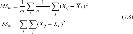
- Mean Square Within, MSw, and Sum of Squares Within, SSw, with MSw being the average of estimates of variances within individual groups,
- Mean Square Between, MSb, and Sum of Squares Between, SSb, with MSb being the estimated variance of means among groups,
- Mean Square Total, MSt, and Sum of Squares Total, SSt, with MSt being the estimated variance of the total mean (ignoring group membership),


The Mean Square Within, SSW, is usually called error variance. The term implies that one cannot readily account for this value in one's data. The Mean Square Between, SSb, usually called effect variance, is due to the difference in means between the groups. Consider the ratio
Under our assumption, this ratio has an F distribution with (m − 1) degrees of freedom in the numerator and (N − m) degrees of freedom in the denominator. Note that MSb is a valid variance estimate only if the null hypothesis is true. Therefore, the ratio is distributed as F only if the null hypothesis is true. This suggests that we can test the null hypothesis by comparing the obtained ratio with that expected from the F distribution. Under the null hypothesis, variance estimated based on the within-group variability should be the same as the variance due to between-group variability. We can compare these two variance estimates using the F test, which checks if the ratio of two variance estimates is significantly greater than 1.
To summarize the basic idea of ANOVA, its purpose is to test differences in the group for statistical significance. This is accomplished by a data variance analysis, namely by partitioning the total variance into a component that is due to the true random error (i.e., SSW) and components that are due to differences between the means (i.e., SSb). These latter components of variance are then tested for statistical significance. If the differences are significant, we reject the null hypothesis (which expects no difference between the means) and accept the alternative hypothesis (that the means in the population differ).
7.4.4 Two-Way Analysis of Variance
Main Effects. One-way analysis of variance handles group data for a single variable. For example, ANOVA can address the effect of visibility by testing differences between the visible group and the invisible group. Nonparametric statistics (Section 7.4.2) can do this as well. Sometimes more than one independent variable (factor) has to be taken into account.
For example, in the Experiment One data, human performance may be determined by the visibility factor and also by the interface factor. One important reason for using the ANOVA method rather than the multiple two-group non-parametric U-test is the efficiency of the former: With fewer observations we can gain more information [126].
Suppose we want to analyze the data in Table 7.8. The two rows in the table correspond to the two levels of factor A, namely, A1, and A2; the two columns correspond to the two levels of factor B, namely, B1 and B2. The levels of factor A can be, for example, the visible group and the invisible group, and the levels of factor B can be the virtual group and the physical group. The cell ABij in the table relates to the level Ai of factor A and the level Bj of factor B, i, j = 1, 2. In general the number of levels of A does not have to be equal to that of B. For simplicity, assume that the number of observations at every level/factor is the same, n.
Here are some notations that we will need:
- I—number of levels of factor A;
- J—number of levels of factor B;
- n —number of observations in each cell ABij;
- N—total number of observations in the entire experiment; hence N = n * I * J;
- μ—unknown population means, as follows:
 —the mean for level i, summed over subscript j,
 —the mean for level j, summed over subscript i,
 —overall mean of all μij,
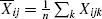 —average within a cell over its subjects' scores,
TABLE 7.8. An Example of a Two-Way Data Layout
 —average for the row i of A over related subjects' scores,
 —average for the column j of B over related subjects' scores,
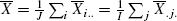 —overall mean of all the scores.
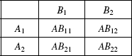
With this notation, if we only test for the main effect of factor B (similarly for the main effect of factor A), the null and alternative hypotheses can be written as
- H0(B): μj = μ for all j
- H1(B): μj ≠ μ for at least one j
The Main Sum Between, ![]() , for J cells of factor B, is the average of estimated variance of estimated column means (this ignoring factor A). That is,
, for J cells of factor B, is the average of estimated variance of estimated column means (this ignoring factor A). That is,
The Main Sum Within is the same error variance MSw considered above; it is equal to the average of (separately estimated) variances within the individual cells. Under the null hypothesis,
That is, the ratio of two main averages has an F distribution with (J − 1) degrees of freedom in the numerator and (N − IJ) degrees of freedom in the denominator, which is the total number of observations N minus the total number of cells, IJ.
Interaction Between Factors. Unfortunately, the main effects are not sufficient to answer questions such as, “Does the effect of factor A remain the same at different levels of factor B?” For example, in some observations of Experiment One the main effect of the visibility factor is that it significantly affects the subjects' path length: The invisible task results in longer path lengths compared to the visible task. However, we notice that the subjects' scores on the visibility factor are also affected by the interface factor: Namely, in the physical test (in the booth) the visibility factor has no significant effect on the path length, whereas in the virtual test the visibility factor has a significant effect on the path length. This suggests that the tests on main effects may be missing such interaction effects. The latter can be tested by the following formulas of interaction (for details refer to Refs. 126 and 127):
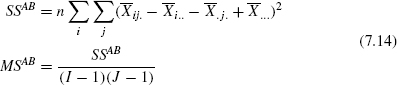
where MSAB represents the Interaction Mean Square between factors A and B. The ratio has an F distribution with (I − 1)(J − 1) degrees of freedom in the numerator and (N − IJ) degrees of freedom in the denominator.
In the case considered now, the results of F test may show that the effect of visibility factor on the path length depends on the type of interface utilized in a given task. In other words, there is an interaction between the visibility factor and the interface factor. One way to express interactions is by saying that one effect is modified (qualified) by another effect.
When the data indicate an interaction between factors, the notion of a main effect has no meaning. In such cases, tests of simple effects can be more useful than tests of main effects. Simple effect tests are done via one-way analysis of variance across levels of one factor, performed separately at each level of the other factor. For example, even if we suspect an interaction between the visibility factor and the interface factor, we might undertake simple effect tests for the visibility factor separately at the virtual and physical level, respectively, and see what kind of conclusions can be made based on the results.
7.4.5 Implementation: Two-Way Analysis for Path Length
We are now ready to perform the analysis of variance on the Experiment One data. From other tests above, we already know that the direction factor has a significant effect on the path length. We know, further, that the left-to-right task is significantly easier for the subjects (it results in shorter paths) than the right-to-left task. We now want to analyze the combined effect of visibility and interface factors on the subjects' performance. Even though the underlying data are not known to obey the normal distribution, we justify using the ANOVA by the F test being known to be robust.
The data set has been first separated into the LtoR and RtoL data sets. The ANOVA variables are:
- Dependent variable: Path length.
- Independent variables:
- Visibility factor, with two levels: visible and invisible.
- Interface factor, with two levels: virtual and physical.
In the tables of results that appear here, the following terms are used:
df effect—degrees of freedom for a given effect, including main and interaction effects.
MS effect—Mean Square for an effect, including main and interaction effects.
df error—degrees of freedom for the error variance, or Mean Square Within.
MS error—Mean Square for the error variance, or Mean Square Within.
Rows with the effect names “1” and “2” correspond to main effects.
Rows with more than one digit in the name, such as “12” or “123,” relate to the corresponding interaction effects.
Results. For the left-to-right task, the summary of ANOVA results appears in Table 7.9. The p-levels for the visibility and interface factors are about 0.01, and the p-level for the interface is much greater than 0.01. This means the main effects of both factors are slightly significant, and there is no interaction. We therefore conclude that for both visible and invisible environments, the path length is affected only slightly by the interface factor. This reconciles with our knowing that for the physical task the path length is slightly shorter than for the virtual task. And, for both physical and virtual tasks the path length is only slightly affected by the visibility factor. Again, this reconciles with our knowing that in the visible environment the path length is slightly shorter than in the invisible environment.
The summary of ANOVA results for the right-to-left task appears in Table 7.10. Here the p-levels for the visibility factor, the interface factor, and the interaction are all greater than 0.01. Therefore, the main effects make no significant difference for the dependent variable, and there is no interaction. The conclusion is that for either the visible or invisible environments, the path length for the physical task is not significantly different from the path length in the virtual task. Also, in either of physical or virtual tasks, the path length in the visible environment does not significantly differ from the path length in the invisible environment.
TABLE 7.9. ANOVA Results for Path Length: Interface and Visibility Factors; LtoR Task
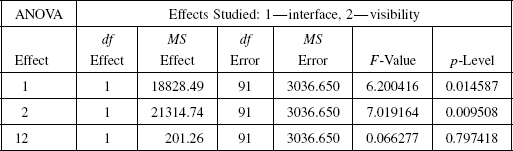
TABLE 7.10. ANOVA Results for Path Length: Interface and Visibility Factors; RtoL Task

7.4.6 Implementation: Two-Way Analysis for Completion Time
In the previous section we have analyzed the effects of test factors on the length of paths generated by the human subjects in Experiment One. We will now analyze how these same factors affect another performance indicator, the task completion time.
Each completion time score is random and independent (for the 48 subjects tested here); this meets the “sampling assumption” of nonparametric statistics and analysis of variance. Even though a closer look at the completion time data shows that they do not obey a normal distribution (as the ANOVA assumption requires), we still use ANOVA, counting on the F test known to be robust.
To analyze the effect of all factors on the completion time data, a three-way analysis of variance has been done. The ANOVA variables are as follows:
- Dependent variable: Completion time.
- Independent variables:
- Direction factor, with two levels: LtoR and RtoL.
- Visibility factor, with two levels: visible and invisible.
- Interface factor, with two levels: virtual (simulation) and physical (booth).
Second, since we are more interested in the visibility factor and interface factor, and since the performance in LtoR task significantly differs from that in RtoL task, a two-way ANOVA was implemented. The ANOVA variables are:
- Dependent variable: Completion time.
- Independent variables:
- Visibility factor, with two levels: visible and invisible.
- Interface factor, with two levels: virtual and physical.
Results. The summary of ANOVA results of analysis of variance for all three factors used in Experiment One appears in Table 7.11. The p-levels for the interface factor, the direction factor, and the interaction between them are less than 0.01. This means that these two main effects likely significantly affect the dependent variable (completion time), and there is interaction between them. The p-levels for the remaining main effect, visibility, and for interactions with this factor are greater than 0.01. This means that there is no significant difference for these effects and interactions. However, given that an interaction has been detected, we should not be forming any conclusions from the results in Table 7.11 until we separate the factor levels.
TABLE 7.11. ANOVA Results for Completion Time: Direction, Interface, and Visibility Factors

TABLE 7.12. ANOVA Results for Completion Time: Interface and Visibility Factors, LtoR Task
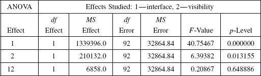
Hence the data for the left-to-right task was analyzed, which is one of two levels of the direction factor. The summary of related ANOVA results appears in Table 7.12. The p-level for the interface factor is smaller than 0.01, the p-level for the visibility factor is about 0.01, and the p-level for the interface factor is greater than 0.01. Therefore, the main effect of interface is statistically significant, the main effect of visibility is slightly significant, and there is no interaction between them. This reconciles with our knowledge that for both visible or invisible tasks, the completion time for the physical task is significantly shorter than for the virtual task. Similarly, for both physical or virtual tasks the completion time is slightly shorter in the visible environment than in the invisible environment.
The summary of ANOVA results for the right-to-left task appears in Table 7.13. The p-level for the interface factor is smaller than 0.01, the p-levels for the visibility factor and interaction are greater than 0.01. This means the main effect of the interface factor is statistically significant, and there is no interaction. This reconciles with test observations: For both visible or invisible tasks the completion time in the physical task was significantly shorter than in the virtual task. Similarly, for both physical and virtual tasks the completion time in the visible environment shows no significant difference from that in the invisible environment.
TABLE 7.13. ANOVA Results for Completion Time: Interface and Visibility Factors, RtoL Task

7.5 RESULTS – EXPERIMENT TWO
Recall that Experiment Two was designed to analyze the effect of subjects' training and the related effect of the visibility factor on human performance. A total of 12 subjects appeared in this study. In the first group, which included six subjects, on day 1 each subject was subjected to six different training tasks, plus one test task at the end, all in the visible environment. About one week later, on day 2, the same subjects performed the same six training tasks, plus the same test task, this time in the invisible environment. In the second group, the remaining six subjects did the same tasks in the opposite order—that is, tests in the invisible environment on day 1 and tests in the visible environment on day 2. The specific task was right-to-left movement of the arm, the same as in Experiment One (recall that this is a more difficult task compared to the left-to-right task).
We therefore have a training factor Day, with two levels, day 1 and day 2. Subjects were expected to learn the motion planning skill through a repeated exercise.
Similar to Experiment One, human performance was measured by the path length and completion time for each of the tasks Path and Time. Path length is the measure of motion generated by the arm manipulator during the task. Completion time is the time it takes the subject to complete the task. Both measure the subjects' proficiency in carrying out motion planning. We suppose that both the path length and the completion time may be affected by such factors as training and visibility of the scene, and we would like to quantify those effects.
In statistical terms, the training and visibility factors are independent variables, whereas the path length and completion time are dependent variables. The objective of data analysis is to test whether the training and/or visibility factor improves the overall human performance in motion planning. If in terms of both dependent variables the improvement in subjects' performance turns out to be significant, follow-up tests on the separate effects on human performance should be conducted, to explain which specific aspects of human performance are responsible for such effects. Multivariate analysis of variance (MANOVA) is a good technique for data analysis of overall effects [128].
Multivariate analysis of variance is conceptually a straightforward extension of the univariate ANOVA technique described above. Their major distinction is that if in ANOVA one evaluates mean differences on a single dependent variable, in MANOVA one evaluates mean vector differences simultaneously on two or more dependent variables. In addition, the MANOVA design accounts for the fact that dependent variables may be correlated. For instance, two dependent variables in Experiment Two, the path length and completion time, are indeed relatively highly correlated, with the correlation coefficient 0.79. In this case, MANOVA should provide a distinct advantage over separate ANOVAs. In fact, performing separate ANOVA tests carries an implicit assumption that either the dependent variables are uncorrelated or such correlations are of no importance.
7.5.1 The Technique
Assumptions. The first and partly second of the three following assumptions are required by MANOVA (and are the same for the statistical tests considered above):
- Observation scores are randomly sampled from the population of interest. Observations are statistically independent of one another.
- Dependent variables have a multivariate normal distribution within each group of interest. This means that (a) each dependent variable is distributed normally, (b) any linear combination of the dependent variables are distributed normally as well; (c) all subsets of the variables have a multivariate normal distribution. In practice, it is unlikely that this and the next assumption are met precisely. Fortunately, similar to ANOVA, MANOVA is relatively robust to violations of these assumptions. In practice, MANOVA tends to perform well regardless of whether or not the data violate these assumptions.
- Homogeneity of covariance matrices. That is, all groups of data are assumed to have a common within-group population covariance matrix. This can be likened to the assumption in ANOVA of homogeneity of variance for each dependent variable, or the assumption that correlation between any two dependent variables must be the same in all groups. If the number of subjects is approximately the same in the experimental groups, a violation of the assumption of covariance matrix homogeneity leads to a slight reduction in statistical power [128–130].
Multivariate Null Hypothesis. Hypotheses in MANOVA are very similar to those in univariate ANOVA, except that vectors of means are considered instead of single values (scalars) of means. For a simple example, imagine we carry out a one-way MANOVA for a visible task and invisible task groups. We would like to know if the scores of path length and completion time came from the same population that includes visible and invisible task data. That is, we want to compare the population mean vector for the dependent variables for one group with the population mean vector for the dependent variables for another group.
Suppose μij represents the mean of the dependent variable i for group j, i = 1, 2, j = 1, 2. The mean vector for group j can be written as
![]()
Then the multivariate null hypothesis H0 can be written as an equality of vectors:
![]()
The alternative hypothesis H1 in this case says that for at least one variable there is at least one group with a population mean different from that in the other group(s):
![]()
Calculating MANOVA Test Statistics. Derivation of the MANOVA test statistics is similar to that in ANOVA but involves relatively cumbersome matrix operations and equations. Hence we will limit the discussion to a conceptual level (see Ref. 130 for more detail).
Recall that the ANOVA attempts to test if the amount of variance explained by the independent variable (namely, SSb, see Section 7.4.3) exceeds significantly the variance that has not been explained (namely, SSw). The variance here is a function of the sum of squares of deviations from the mean for an entire group (the latter being called the sum of squares, SS). The ANOVA's F statistics is a ratio of the mean square between, MSb, to the mean square within, MSw.
Instead of scalars of dependent variables, MANOVA employs a vector of dependent variables. A single sum of squares is replaced with a complete (total) matrix of sums of squares and cross-products, SPt. Along its diagonal the matrix has the sums of squares that represent variances for all dependent variables, and in its off-diagonal elements it has cross-products that represent covariances of variables. Just as a univariate ANOVA, MANOVA divides matrix SPt into the within-group matrix, SPw, and the between-group matrix, SPb. From algebra, the matrix determinant expresses the amount of generalized variance, or the total variability that is present in the underlying data and is expressed through the dependent variables. One can hence compare the generalized variance of one matrix with another.
Wilks' lambda test is perhaps the most widely used statistical test of multivariate mean differences [130]. It derives from the following idea. Since matrix SPb represents the amount of explained variance and covariance, and matrix SPw represents the remaining variance and covariance, in the case of a significant effect one would expect matrix SPb to have a larger generalized variance compared to matrix SPw. Wilks' lambda index, ∧, is defined as a ratio of determinants of the two matrices:
where SPt, SPw, and SPb are the total, within-group, and between-group SP matrices, respectively.
We associate the value of ∧ with the effect's significance. The value can also be interpreted as the proportion of unexplained variance. The main effects and interaction effects in multiple-way MANOVA are conceptually the same as those in ANOVA. While computations are more complex in MANOVA, their underlying logic is the same as in ANOVA.
If an overall significant multivariate effect is found, the next natural step is to submit the data to further testing, to see whether all dependent variables or some specific dependent variables are affected by the independent variables. Performing multiple univariate ANOVAs for each of the dependent variables is a common method for interpreting the respective effects. One attempts to identify specific dependent variables that contributed to the overall significant effect.
Repeated Measures MANOVA. In our statistical tests so far, all independent variables involved in ANOVA and MANOVA were also between-subjects variables (or factors); we were interested in differences between means or mean vectors of several distinct groups of subjects. The observed scores were independent of each other at different levels of the between-subjects variables.
However, in Experiment Two we also want to study the difference in responses of the same subjects before and after treatment; in our case, treatment is training. This variable is called repeated measures, and its analysis is called repeated measures MANOVA. In a repeated measures design the several response variables are results of the same test carried out by the same subjects, applied a number of times or under more than one experimental condition. For example, in Experiment Two each subject was assessed as to their path length and completion time on day 1 and again on day 2. The variable “day” is a repeated measures variable, as well as a within-subjects variable.
In other words, a between-subjects variable is a grouping variable—similar to the visibility or interface in our study—whereas a within-subjects variable refers to the measurements for every level of the within-subjects variable. For example, a within-subjects variable may be “time,” or “day,” or “training factor.” A study can involve both within- and between-subjects independent variables. Our Experiment Two analysis constitutes a 2 (days) by 2 (visibility levels) repeated measures MANOVA, or repeated measures ANOVA. The first independent variable, day, is a within-subjects (repeated measures) variable, and the last independent variable, visibility, is a between-subjects variable.
Repeated measures MANOVA is an extension of the standard MANOVA. The underlying principles of both are almost the same. In the standard MANOVA, vectors of means are compared across the levels of independent variables. In the repeated measures MANOVA, vectors of mean differences are compared across the levels of independent variables.
Mean differences are the differences in values of dependent measures between levels of the within-subjects variable. These can be seen as new independent variables. If, for example, the dependent variables were measured for each subject at four different time moments, say at times T1 through T4, these original four variables would be transformed to three alternative derived difference variables, denoted (T1–T2), (T2–T3), and (T3–T4). These three new variables directly address the questions of interest. The repeated measures MANOVA, therefore, compares the vectors of means across the new transformed variables, not the original scores.
When conducting a repeated measures MANOVA, a sphericity assumption must be met. It requires that the covariance matrix for the transformed variables be a diagonal matrix. That is, the values (variances) along the diagonal of the transformed covariance matrix should be equal, and all the off-diagonal elements (correlation coefficients) should be zeros. The purpose of the sphericity assumption is to ensure the homogeneity of covariance matrices for the new transformed variables [131, 132].
7.5.2 Implementation Scheme
Experiment One. Recall that in Experiment One the observation scores in each task were measured on two dependent variables, path length and completion time. Subjects have been randomly selected, and sets of scores were mutually independent. Further, the two dependent variables were correlated, with the correlation coefficient 0.74. We take this correlation into account when performing the significance test, since the overall set of dependent variables may contain more information than each of the individual variables. This suggests that the Experiment One data can be a candidate for a multivariate analysis of variance, MANOVA.
Since, as discussed in the previous section, the effect of direction factor in Experiment One is statistically significant, we separately perform two sets of MANOVAs—one for the left-to-right task and the other for the right-to-left task. When performing MANOVA for the left-to-right task, the data set forms a two-way array, 2 (visibility) × 2 (interface). For the right-to-left task, the data set also forms a two-way array, 2 (visibility) × 2 (interface). The results of analysis should answer questions such as: (1) does human performance improve in the visible environment compared to the invisible environment? (2) Does human performance improve in a test with the physical arm manipulator as compared to the virtual arm manipulator? (3) Does the effect of the visibility factor work across the levels of the interface factor?
TABLE 7.14. Descriptive Statistics for the Data in Experiment Two

Experiment Two. Table 7.14 lists basic descriptive statistics for the Experiment Two data: the number N of valid observations in each group; and means, minimums, maximums, and standard deviations in each group. In the table, “vis” means visible, “invis” means invisible, “path” means path length, and “time” means task completion time.
Similar to Experiment One, the Experiment Two data for each task were recorded for two dependent variables, path length and completion time. Subjects were randomly selected, and the sets of scores were independent of each other. The correlation coefficient of the two dependent variables is 0.79. This correlation suggests that each dependent variable contains some new information as well as some information overlapping with the other dependent variables. Accounting for this correlation allows us to test the significance of dependent variables in human performance. Since the data in Experiment Two correspond to the same subjects on day 1 and day 2, the day factor is a repeated measures variable with two levels, day 1 and day 2. These data call for a repeated measures MANOVA.
The Experiment Two data form a two-way array, 2 (day) × 2 (visibility). If any main effects or interaction effects are identified, multiple univariate ANOVA would be performed, in order to observe the effects on each dependent variable. In our data analysis we are interested in these questions: (1) Is there an improvement in human performance across day 1 and day 2? (2) Is there a statistically significant difference in human performance in the visible as opposed to invisible environment? and (3) Does the effect of one independent variable change over the levels of another independent variable?
Combined Experiment One and Two. There is another data set that we can use to test the effects of training and visibility. The first half of the data (12 subjects) in this new combined data set was extracted from the Experiment One. Six of these were randomly picked among the virt–vis–RtoL data, and another six were randomly picked among the virt–invis–RtoL data. The second half (12 subjects) of the data in the new combined set are the day 2 data (12 subjects) from Experiment Two.
The purpose of MANOVA or ANOVA analysis on this combined data set is to test whether human performance would show improvement from day 0, when the subjects executed tasks without any training (in Experiment One), to day 2, when subjects had a benefit of several training trials (in Experiment Two). The effect of visibility would also be tested here. Note, however, that the day factor in this analysis is not a repeated measure variable any longer but instead a between-subjects variable. This is because there are no pairs of data for day 0 and day 2 coming from the same subjects (which would be required by the definition of repeated measure variable). The data for day 0 are independent with respect to the data for day 2. Therefore, the new combined data form a two-way array, 2 (day) × 2 (visibility).
7.5.3 Results and Interpretation
1. The MANOVA scheme was applied to the left-to-right data in Experiment One. The variables involved are as follows:
- Dependent variables:
- Path length.
- Completion time.
- Independent variables:
- Interface, with 2 levels: virtual and physical.
- Visibility, with 2 levels: visible and invisible.
The results are shown in Table 7.15. Here df is the degrees of freedom (see Section 7.4.5). Note that the p-level for interaction between the two independent variables is significantly high. We thus conclude that there is no interaction effect. This means that the effect of one independent variable does not change across the levels of the other independent variable. The p-level for the interface factor is almost zero. We therefore reject the null hypothesis of the MANOVA, and we conclude that the interface factor has a statistically significant effect on the overall human performance. The p-level for the visibility factor shows that the overall human performance is only slightly improved in the visible environment compared to the invisible environment.
TABLE 7.15. Results of MANOVA for LtoR Task, Experiment One

Given a significant effect indicated by the MANOVA results, multiple univariate ANOVAs have followed.
2. The MANOVA was applied to the right-to-left data in Experiment One. The variables are as follows:
- Dependent variables:
- Path length.
- Completion time.
- Independent variables:
- Interface, with 2 levels: virtual and physical.
- Visibility, with 2 levels: visible and invisible.
The results are shown in Table 7.16. Note that the p-level for the interaction effect between the two independent variables is large enough; we can conclude that there is no interaction effect. This means that the effect of one independent variable is not influenced by the other independent variable. The p-level for the interface factor is almost zero, hence we reject the null hypothesis of MANOVA. That is, the interface factor has a statistically significant effect on the overall subjects' performance. The p-level for the visibility factor is large; we thus conclude that the overall subjects' performance was affected by the visibility factor.
Since a significant effect was demonstrated by this MANOVA, multiple uni-variate ANOVAs have followed.
3. MANOVA was applied to the Experiment Two data. The variables involved are as follows:
- Dependent variables:
- Path length.
- Completion time.
TABLE 7.16. Results of MANOVA for RtoL Task, Experiment One

TABLE 7.17. Results of MANOVA, Experiment Two
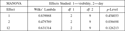
- Independent variables:
- Visibility, with 2 levels: visible and invisible.
- Day (repeated measures), with 2 levels: day 1 and day 2.
The results are shown in Table 7.17. The p-level for the interaction effect is bigger than the significance level (0.05), pointing to no significant interaction effect. This means the result for one independent variable is not modified by the other independent variable. The p-level for the visibility factor is also larger than the significance level, so the null hypothesis should be accepted. In other words, the overall human performance is not affected by the visibility factor. The p-level for the day factor suggests a slight effect of the day (training) factor on human performance. This reconciles with our knowing that the overall subjects' performance was better on day 2 compared to day 1.
In order to see which indicator of human performance might be affected by the day (training) factor, multiple univariate ANOVAs have been performed.
4. ANOVA was applied to the path-length-dependent variable in Experiment Two. The variables involved are as follows:
- Dependent variables:
- Path length.
- Independent variables:
- Visibility, with two levels: visible and invisible.
- Day (repeated measures), with two levels: day 1 and day 2.
The results are shown in Table 7.18. The p-levels for the main effects and interaction effect are larger than the significance level 0.05. Each null hypothesis for the main effects and interaction effect should hence be accepted. We conclude that there are no significant effects of the visibility factor and day (training) factor, and that these results do not change across the levels of the independent variables. In other words, surprisingly, the visibility factor has no significant effect on the subjects' path length, and the day (training) effect has no significant effect on the path length as well.
TABLE 7.18. Results of ANOVA for Path Length, Experiment Two
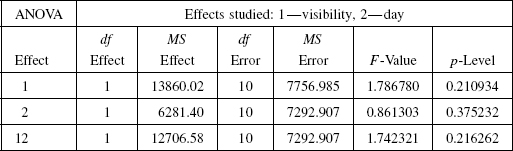
TABLE 7.19. Results of ANOVA on Completion Time, Experiment Two
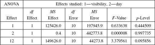
5. An ANOVA was applied to the independent variable of completion time in Experiment Two. The variables involved are as follows:
- Dependent variables:
- Completion time.
- Independent variables:
- Visibility, with 2 levels: visible and invisible.
- Day (repeated measures), with 2 levels: day 1 and day 2.
The results are shown in Table 7.19. The p-levels for the main effects and interaction effect are all larger than the accepted threshold significance level 0.05. Hence all null hypotheses for the main effects and interaction effect are accepted. We thus conclude that there are no significant effects for the visibility factor and day (training) factor, and this does not change across all levels of the independent variables. In other words, surprisingly, neither the visibility factor nor the day (training) factor has a significant effect on the completion time.
6. The MANOVA was applied to the combined data set. The variables involved are as follows:
- Dependent variables:
- Path length.
- Completion time.
TABLE 7.20. Results of MANOVA in the Combined Data Set

- Independent variables:
- Visibility, with 2 levels: visible and invisible.
- Day (repeated measures), with 2 levels: day 0 and day 2.
The results are shown in Table 7.20. Note that the p-level for the interaction effect is larger than the significance level. We therefore conclude that there is no interaction effect in these data, and hence any main effect is not modified across the levels of another main effect. The p-levels for the day factor and visibility factor are large enough, so the null hypotheses for these main effects are accepted. This means that both the day (training) factor and the visibility factor do not improve the overall human performance; that is, subjects' path lengths and completion times are not improved (decreased) by providing them with a visible environment or with the opportunity to train and practice.
7.6 DISCUSSION
The study described in this chapter focuses on experimental testing of human performance in tasks that deal with motion planning and require spatial reasoning. The experimental stage was followed with a thorough statistical analysis of the obtained test data. As said in the introduction to this chapter, the motivation for the study was two-prong. First, we wanted to use these data to compare human performance with the performance of robot sensor-based motion planning algorithms described elsewhere in this book. Second, we wanted to foresee the human performance in robot teleoperation systems, with an eye on techniques to compensate for operator deficiencies via a synergistic human–robot operation. To recap our prior discussion, assessing robot motion planning algorithms raises these questions:
- The question of quality of sensor-based robot motion planning algorithms can in principle be addressed in a number of ways. As those options are listed below, we will note that the last option—a comparison with human performance—stand out as more attractive:
— One can compare actual generated paths with optimal paths. This comparison would make, however, little sense simply because producing an optimal path requires complete information about the environment whereas our algorithms have only limited sensing information.
— One can assess algorithms' performance theoretically. We have done this in Chapter 3 for the case of a point robot moving in the plane. The upper bounds on the robot performance obtained there give a good idea about the worst-case performance of the algorithms, but they do not answer the direct practical “How good is it in ‘normal life’ ?” question.
— One can attempt a comparison between paths produced by different algorithms in the same task. While some such comparisons have been done in literature, they are of limited value simply because different algorithms tend to behave differently in different tasks: An algorithm that wins in one task can easily lose in another task. That is why the task of choosing between algorithms is a hard one. And, importantly, such a comparison is not feasible for arm manipulators because today there is no competing options to the sensor-based algorithms developed in Chapters 5 and 6.
— One can compare the algorithms' performance with human performance. While we still don't know what algorithms people use in such tasks, from the practical standpoint this would be a satisfying comparison. After all, we humans do solve motion planning problems with uncertainty. We do it all the time, and so using human performance as a benchmark would be an “apples-to-apples” comparison. We tend to associate motion planning tasks with “thinking” and intelligence: If our robots perform well in such tasks, we not only can be proud of the robots' performance but can also use this fact in technical systems.
- If human performance in motion planning tasks turns out to be less than ideal—and the results described in this chapter demonstrate that this is so for tasks with arm manipulators—this conclusion should pose a serious challenge to designers of practical human-guided teleoperation systems. If robot skills in motion planning are better than human skills, and if that is still so after a substantial training by humans, this becomes a good argument for a new design approach in teleoperation systems. Namely, we should attempt to switch to human–robot synergy teams, where human intelligence is complemented with appropriate robot intelligence.
In our tests the performance of human subjects was measured in terms of two dependent variables:
- Path length— the length of paths a subject generates in a given task.
- Task completion time— the time a subject takes to complete a given task.
The experimental data appear in groups, each related to one independent variable (factor). Overall, four factors have been studied:
- Task Interface: Each subject operated either a virtual arm manipulator on the computer screen or a physical arm in the test booth.
- Visibility of the Scene: The subject either was given a bird's-eye view of the scene or was forced to “move in the dark.”
- Direction of the arm motion in the scene (this factor had played an auxiliary role in the study): When moving the arm manipulator, the subject had to move it either from “start” to “target” position or in the opposite direction.
- Training factor represented by specific days on which the test was taken: Namely, on day 1 the subjects had moved the arm after only a small perfunctory practice; on day 2 they had a benefit of significant prior training.
The summary of results of statistical processing of testing data appears in Table 7.21 (here, “no” means “no effect”; the corresponding details appear in Sections 7.4.6 and 7.5.3). The table shows effects of each factor on the overall human performance and on each component of human performance, path length and completion time.
TABLE 7.21. Summary of Results in Experiments One and Two

The motion direction factor is not included in the table since it was added to the study only as a secondary factor, to shed light on the primary factors' effects.
In brief, statistical analysis of experimental data from tests with arm manipulator motion planning indicates the following:
- The interface factor has no significant effect on the length of generated paths, but has a significant effect on the task completion time.
- The visibility factor has no significant effect on human performance—neither on the path length nor on the completion time.
- Similarly, the training factor has no significant effect on the human performance.
- The motion direction factor has a statistically significant effect on human performance.
Overall, these conclusions look rather surprising. Let us discuss these findings and their implications in more detail.
Effects of the Interface Factor. The two components of this factor are the virtual (simulated) interface and the physical (arm in the booth) interface. Simple considerations and expert opinions suggest that this factor should be of much importance. After all, we humans are used to moving physical objects. Manipulating a physical object—here the arm—adds significant haptic, visual, and even auditory information about the task. Plus, the physical arm looks much like a human arm and hence adds to one's confidence. On the other hand, moving an abstract object on the screen seems far less natural. A good many observers and participants in this study had predicted that the subjects would do much better when moving the physical arm than when moving the virtual arm on the screen.
Indeed, statistical analysis of test data agrees to some extent with this intuition: For the task completion time it does show an improvement in subjects' performance. On the average, subjects moved the physical arm in a more continuous fashion, whereas in the simulation they often paused after small motions, spending extra time on figuring out what to do next.
However, an interesting result here was that the improvement was very small in the path length, and that even this small effect was erased by the motion direction factor: In Table 7.21, column “Effect on Path,” observe those “slight” and “no” (effect) in the ANOVA left-to-right and in ANOVA right-to-left, respectively. The fact that no significant effect of the interface factor on the path length was found in the more difficult right-to-left task is surprising. It suggests that the importance to a human operator of the type of interface fades as the spatial tasks become harder. To put it bluntly, in nontrivial teleoperation motion planning tasks the operators will likely need help, such as from the robot intelligence; mere improvements in the control means will not go far enough.
The difference in the factor effects on the two dependent variables—path length and completion time—is not hard to explain. The length of a path generated by a human subject is, in general, independent of how quickly or slowly one moves the arm or how continuous its motion is. If the subject stops to think how to proceed, this in itself will not increase the path length, but it will increase the time to task completion. The harder the task, the more thinking the operator needs, and the more time he or she takes to think. The relation of task hardness to the length of path is hence more subtle than its relation to the time to completion. This may be a useful consideration for balancing advantages and disadvantages of virtual versus physical control means in real-world teleoperation systems.
Effects of the Visibility Factor. This factor refers to the obstacles in the environment being visible or invisible to the subjects during the test. The test subjects themselves, researchers, and practicing operators usually think that seeing the robot surroundings would significantly improve their performance.
Interestingly, our study suggests that while this common sense judgment applies to very easy tasks, it does not apply to relatively complex tasks. For the easier task in this study (which is moving the arm left-to-right), there is only a slight difference in the resulting path length and completion time. That is, seeing the environment helped a little in path length and in completion time. On the other hand, for the more difficult task (moving the arm right-to-left,) there was almost no difference in the path length and completion time. This looks puzzling, but becomes less so if one considers that many studies have demonstrated that humans are, in general, not very good in spatial reasoning based on visual data. This fact questions the large resources that are often allocated in telerobotics to help the operator see the scene. It also implies that the operator performance is affected less by the visibility factor than by the human spatial reasoning abilities.
Effects of the Training Factor. This factor has two components that refer to the day of the task execution: day 1, before training, and day 2, after training. When comparing human performance on those two days, with the other conditions fixed, any statistically significant difference should be attributed to the effect of training. Namely, a significant difference would support a common wisdom hypothesis that one's performance should improve significantly after learning from repeated exercise.
This study shows that in arm manipulator motion planning tasks, training has no significant effect on human performance, neither in terms of path length nor in the task completion time. In our tasks the subjects were unable to seriously improve their motion planning skills via training. This is no doubt very surprising. One would expect the opposite conclusion: We all know examples of tasks involving motion where, given enough training, humans become extremely adept; an acrobat on the trapeze is but one example.
There is a big difference, however: The acrobat does a once-and-for-all learned motion, whereas our tasks require constant spatial reasoning. Our test protocols do not allow a subject to simply memorize a task. We want our subjects to learn how to do a class of tasks; we want them to improve their spatial reasoning skills, rather than memorize a specific motion. Examples of positive effect of training in tasks that involve spatial reasoning are harder to come up with. Note that since the tasks given to subjects in this study are quite close to teleoperation tasks, the reported results should be taken seriously by designers of teleoperated systems.
There was one exception from this pattern: The training factor had a slight positive effect on the subjects' overall performance in Experiment Two (see the box “Experiment Two and combined data,” Table 7.21; the extent of improvement is only 3.67%). The meaning of this exception is not clear. Given that the effect disappears for the combined Experiments One + Two data (further in the same box in Table 7.21), the small effect of the training factor for the Experiment Two data might be an artifact due to the insufficient data or measurement errors. Or, training may indeed improve—though only a little bit—human performance in motion planning tasks such as ours.
Effects of the Motion Direction Factor. This factor has two components, left-to-right direction and right-to-left direction of motion. These two tasks took place in the same scene and with the same two-link arm manipulator. The only difference was that in the first task one was asked to move the arm from position S (start) to position T (target) (Figure 7.5, Section 7.2.2), and in the second task one would go from T to S. In this study the motion direction factor happened to have a significant effect on the subjects' performance. In fact, the effect has been stronger than other effects observed. Hence the motion direction factor was included in the study, to help assess the effect of the task difficulty on one's performance, with or without other factors involved.
Using the same scene and the same arm in both tasks has an added advantage that the perceived difficulty of one task over the other is then known to be “in one's head only.” After all, a human subject could in principle produce exactly the same path in both tasks, which is what a robot algorithm would do.12 The unequal difficulty of the two tasks as perceived by the subjects is very interesting. It suggests that human performance is limited by human motion planning skills no less than by the task's objective complexity. As a minimum, it demonstrates a profound qualitative difference between the human and robot algorithms.
Why do human subjects perceive the above two tasks as completely different? It is as if changing the direction of motion to right-to-left produces some additional, if unclear, difficulties; perhaps it adds more possibilities for motion planning or more ways to make mistakes. In Section 7.2.3 we made an attempt to speculate about the reasons affecting human performance in these two tasks (see design comment No. 4 and Figure 7.9).
To summarize, in tasks that involve spatial reasoning and motion planning for a multilink kinematic structures, human performance changes surprisingly little with the change in external conditions, such as interface, environment visibility, and training factors:
- Common wisdom suggests that seeing the complete scene should significantly help the operator. This study shows that it is not so, at least for more or less complex tasks.
- Common wisdom suggests that moving a physical device in physical space, rather than moving an equivalent abstract object on the computer screen, should significantly help the operator. This study shows that it is not the case. As the only exception, a slightly shorter completion time was achieved with the physical arm manipulator compared to the simulated manipulator. In other words, the subjects made decisions faster with the physical arm, but this did not improve the paths they produced.
- Common wisdom suggests that training should help operators in improving their performance. This study shows that at least within the training protocol of this study (which is a typical protocol in cognitive science experiments), human performance changed very little with training.
The study suggests that unlike factors that common wisdom expects to be influential in human performance (visibility, interface, training), some other “strange” factors, such as a change in the required direction of motion, may have a much stronger effect. One is left with a thought that we humans have not been designed by nature to handle motion planning tasks with objects that have lengths and joints. That, for example, finding one's place in a forest or in an unknown terrain was so essential for one's survival (note a similarity with the point-robot-in-the-maze problem) that the evolution has built appropriate intelligent strategies in our genes for this task. And that the need for moving kinematic structures—objects with lengths and joints—was not nearly as essential.
Thus today not only don't we have such skills, but we find it very difficult to acquire them. This should not be much of a surprise: We know, for example, that evolution made us capable of learning languages with unbelievable ease at a young age but made this same task excruciatingly difficult at an older age. Well, one may say, at least in languages there is the right age. True, there seems to be no right age for learning how to move kinematic structures. Then, we may want to delegate this job to robots, especially if robots can do it better, as shown in prior chapters.
The results described in this chapter look too strange to leave them unchallenged. We need more controlled experiments with human subjects. We need to understand which kind of tasks are harder and which are easier for human operators. As was done in our study, this work requires a collaboration between system designers and cognitive scientists. This will be especially important if projects of critical importance are entertained. As an example, the announced (in 2004) NASA program to create technology that will allow bringing humans to the moon and later to Mars and beyond has a provision for many highly roboticized tasks, in both autonomous and teleoperation robotic settings. Elucidation of the phenomena addressed in this chapter—in particular, the humans' cognition difficulties with spatial reasoning—will likely have a serious effect on design of robotic systems.
One likely practical design strategy coming out of such studies calls for dividing responsibilities between human and robot intelligence, so that both types of intelligence will control the system simultaneously and in a synergistic manner (see, e.g., Ref. 133).
1Much of the software for this first stage and many tests were produced by my graduate students, especially by Timothy Skewis. The human subjects used were whoever passed through the Yale Robotics Laboratory—graduate students, secretaries, unsuspecting scientists coming to Yale for a seminar, and even faculty's children.
2Of course, in a more complex labyrinth a quick look may not be sufficient to see the solution; then one's performance may deteriorate. For the point that we are to make in this section, this fact is not essential.
3The experimental setup used in Figure 7.6c slightly differs from the other two; this played no visible role in the test outcomes.
4The term “average” here has no formal meaning: It signifies only that some subjects did better and some did worse. A more formal analysis of human performance in this task will be given in the next section. A few subjects did not finish the test and gave up, citing tiredness or hopelessness (“There is no solution here”, “You cannot move from S to T here”…).
5Of course, no such effect can be expected for the computer algorithm.
6An “unscientific” observation made here was that older subjects, such as visiting professors who graciously agreed to participate in the experiment, were more critical of the human–computer interface than younger subjects. The latter were more willing than the former to accept the test results as measuring their real spatial reasoning abilities.
7The physical arm and the booth system, including hardware, electronics, and related software, have been designed by Branimir Stankovic and Steve Seaney at the University of Wisconsin Robotics Laboratory [120].
8In addition to this arm, a wooden mockup of the arm, of the same dimensions as the test arm, was built and installed outside the booth, to help subjects practice their motor skills in the task.
9More details on the experiment design and test conditions can be found in Ref. 121.
10This alone would make a smart robot conclude that we humans are terribly inconsistent: What prevents one, the robot would think, from going from point B to point A along the same path one takes when going from A to B!
11Also, according to the central limit theorem, if the sample size is fairly large, deviations from normality do not matter much [126].
12Formally, this is not exactly so. For example, in the example in Figure 3.5, Section 3.3.2, the path shown from point S to point T is produced using the local direction “left.” If the same algorithm (here Bug2) now starts from T toward S, using the same local direction, the resulting path will be different from the one shown: It will be complementary to the shown path in that it will pass around parts of obstacles that were not passed when moving from S to T. The same is true for the arm manipulator algorithms discussed in Chapters 5 and 6. The nature of this difference is, however, not the same as in human performance. By simply switching the algorithm's local direction to its opposite, we will obtain a path identical to the one shown in Figure 3.5. Whatever rules guide human motion planning strategies, they must be very different.
Sensing, Intelligence, Motion, by Vladimir J. Lumelsky
Copyright © 2006 John Wiley & Sons, Inc.