 CHAPTER 3
Motion Planning for a Mobile Robot
Thou mayst not wander in that labyrinth; There Minotaurs and ugly treasons lurk.
— William Shakespeare, King Henry the Sixth
What is the difference between exploring and being lost?
— Dan Eldon, photojournalist
As discussed in Chapter 1, to plan a path for a mobile robot means to find a continuous trajectory leading from its initial position to its target position. In this chapter we consider a case where the robot is a point and where the scene in which the robot travels is the two-dimensional plane. The scene is populated with unknown obstacles of arbitrary shapes and dimensions. The robot knows its own position at all times, and it also knows the position of the target that it attempts to reach. Other than that, the only source of robot's information about the surroundings is its sensor. This means that the input information is of a local character and that it is always partial and incomplete. In fact, the sensor is a simple tactile sensor: It will detect an obstacle only when the robot touches it. “Finding a trajectory” is therefore a process that goes on in parallel with the journey: The robot will finish finding the path only when it arrives at the target location.
We will need this model simplicity and the assumption of a point robot only at the beginning, to develop the basic concepts and algorithms and to produce the upper and lower bound estimates on the robot performance. Later we will extend our algorithmic machinery to more complex and more practical cases, such as nonpoint (physical) mobile robots and robot arm manipulators, as well as to more complex sensing, such as vision or proximity sensing. To reflect the abstract nature of a point robot, we will interchangeably use for it the term moving automaton (MA, for brevity), following some literature cited in this chapter.
Other than those above, no further simplifications will be necessary. We will not need, for example, the simplifying assumptions typical of approaches that deal with complete input information such as approximation of obstacles with algebraic and semialgebraic sets; representation of the scene with intermediate structures such as connectivity graphs; reduction of the scene to a discrete space; and so on. Our robot will treat obstacles as they are, as they are sensed by its sensor. It will deal with the real continuous space—which means that all points of the scene are available to the robot for the purpose of motion planning.
The approach based on this model (which will be more carefully formalized later) forms the sensor-based motion planning paradigm, or, as we called it above, SIM (Sensing–Intelligence–Motion). Using algorithms that come out of this paradigm, the robot is continuously analyzing the incoming sensing information about its current surroundings and is continuously planning its path. The emphasis on strictly local input information is somewhat similar to the approach used by Abelson and diSessa [36] for treating geometric phenomena based on local information: They ask, for example, if a turtle walking along the sides of a triangle and seeing only a small area around it at every instant would have enough information to prove triangle-related theorems of Euclidean geometry. In general terms, the question being posed is, Can one make global inferences based solely on local information? Our question is very similar: Can one guarantee a global solution—that is, a path between the start and target locations of the robot—based solely on local sensing?
Algorithms that we will develop here are deterministic. That is, by running the same algorithm a few times in the same scene and with the same start and target points, the robot should produce identical paths. This point is crucial: One confusion in some works on robot motion planning comes from a view that the uncertainty that is inherent in the problem of motion planning with incomplete information necessarily calls for probabilistic approaches. This is not so.
As discussed in Chapter 1, the sensor-based motion planning paradigm is distinct from the paradigm where complete information about the scene is known to the robot beforehand—the so-called Piano Mover's model [16] or motion planning with complete information. The main question we ask in this and the following chapters is whether, under our model of sensor-based motion planning, provable (complete and convergent are equivalent terms) path planning algorithms can be designed. If the answer is yes, this will mean that no matter how complex the scene is, under our algorithms the robot will find a path from start to target, or else will conclude in a finite time that no such path exists if that is the case.
Sometimes, approaches that can be classified as sensor-based planning are referred to in literature as reactive planning. This term is somewhat unfortunate: While it acknowledges the local nature of robot sensing and control, it implicitly suggests that a sensor-based algorithm has no way of inferring any global characteristics of space from local sensing data (“the robot just reacts”), and hence cannot guarantee anything in global terms. As we will see, the sensor-based planning paradigm can very well account for space global properties and can guarantee algorithms' global convergence.
Recall that by judiciously using the limited information they managed to get about their surroundings, our ancestors were able to reach faraway lands while avoiding many obstacles, literally and figuratively, on their way. They had no maps. Sometimes along the way they created maps, and sometimes maps were created by those who followed them. This suggests that one does not have to know everything about the scene in order to solve the go-from-A-to-B motion planning problem. By always knowing one's position in space (recall the careful triangulation of stars the seaman have done), by keeping in mind where the target position is relative to one's position, and by remembering two or three key locations along the way, one should be able to infer some important properties of the space in which one travels, which will be sufficient for getting there. Our goal is to develop strategies that make this possible.
Note that the task we pose to the robot does not include producing a map of the scene in which it travels. All we ask the robot to do is go from point A to point B, from its current position to some target position. This is an important distinction. If all I need to do is find a specific room in an unfamiliar building, I have no reason to go into an expensive effort of creating a map of the building. If I start visiting the same room in that same building often enough, eventually I will likely work out a more or less optimal route to the room—though even then I will likely not know of many nooks and crannies of the building (which would have to appear in the map). In other words, map making is a different task that arises from a different objective. A map may perhaps appear as a by-product of some path planning algorithm; this would be a rather expensive way to do path planning, but this may happen. We thus emphasize that one should distinguish between path planning and map making.
Assuming for now that sensor-based planning algorithms are viable and computationally simple enough for real-time operation and also assuming that they can be extended to more complex cases—nonpoint (physical) robots, arm manipulators, and complex nontactile sensing—the SIM paradigm is clearly very attractive. It is attractive, first of all, from the practical standpoint:
- Sensors are a standard fare in engineering and robot technology.
- The SIM paradigm captures much of what we observe in nature. Humans and animals solve complex motion planning tasks all the time, day in and day out, while operating with local sensing information. It would be wonderful to teach robots to do the same.
- The paradigm does away with complex gathering of information about the robot's surroundings, replacing it with a continuous processing of incoming sensor information. This, in turn, allows one not to worry about the shapes and locations of obstacles in the scene, and perhaps even handle scenes with moving or shape-changing obstacles.
- From the control standpoint, sensor-based motion planning introduces the powerful notion of sensor feedback control, thus transforming path planning into a continuous on-line control process. The fact that local sensing information is sufficient to solve the global task (which we still need to prove) is good news: Local information is likely to be simple and easy to process.
These attractive points of sensor-based planning stands out when comparing it with the paradigm of motion planning with complete information (the Piano Mover's model). The latter requires the complete information about the scene, and it requires it up front. Except in very simple cases, it also requires formidable calculations; this rules out a real-time operation and, of course, handling moving or shape-changing obstacles.
From the standpoint of theory, the main attraction of sensor-based planning is the surprising fact that in spite of the local character of robot sensing and the high level of uncertainly—after all, practically nothing may be known about the environment at any given moment—SIM algorithms can guarantee reaching a global goal, even in the most complex environment.
As mentioned before, those positive sides of the SIM paradigm come at a price. Because of the dynamic character of incoming sensor information—namely, at any given moment of the planning process the future is not known, and every new step brings in new information—the path cannot be preplanned, and so its global optimality is ruled out. In contrast, the Piano Mover's approach can in principle produce an optimal solution, simply because it knows everything there is to know.1 In sensor-based planning, one looks for a “reasonable path,” a path that looks acceptable compared to what a human or other algorithms would produce under similar conditions. For a more formal assessment of performance of sensor-based algorithms, we will develop some bounds on the length of paths generated by the algorithms. In Chapter 7 we will try to assess human performance in motion planning.
Given our continuous model, we will not be able to use the discrete criteria typically used for evaluating algorithms of computational geometry—for example, assessing a task complexity as a function of the number of vertices of (polygonal or otherwise algebraically defined) obstacles. Instead, a new path-length performance criterion based on the length of generated paths as a function of obstacle perimeters will be developed.
To generalize performance assessment of our path planning algorithms, we will develop the lower bound on paths generated by any sensor-based planning algorithm, expressed as the length of path that the best algorithm would produce in the worst case. As known in complexity theory, the difficulty of this task lies in “fighting an unknown enemy”—we do not know how that best algorithm may look like.
This lower bound will give us a yardstick for assessing individual path planning algorithms. For each of those we will be interested in the upper bound on the algorithm performance—the worst-case scenario for a specific algorithm. Such results will allow us to compare different algorithms and to see how far are they from an “ideal” algorithm.
All sensor-based planning algorithms can be divided into these two nonoverlapping intuitively transparent classes:
Class 1. Algorithms in which the robot explores each obstacle that it encounters completely before it goes to the next obstacle or to the target.
Class 2. Algorithms where the robot can leave an obstacle that it encounters without exploring it completely.
The distinction is important. Algorithms of Class 1 are quite “thorough”—one may say, quite conservative. Often this irritating thoroughness carries the price: From the human standpoint, paths generated by a Class 1 algorithm may seem unnecessarily long and perhaps a bit silly. We will see, however, that this same thoroughness brings big benefits in more difficult cases. Class 2 algorithms, on the other hand, are more adventurous—they are “more human”, they “take risks.” When meeting an obstacle, the robot operating under a Class 2 algorithm will have no way of knowing if it has met it before. More often than not, a Class 2 algorithm will win in real-life scenes, though it may lose badly in an unlucky scene.
As we will see, the sensor-based motion planning paradigm exploits two essential topological properties of space and objects in it—the orientability and continuity of manifolds. These are expressed in topology by the Jordan Curve Theorem [57], which states:
Any closed curve homeomorphic to a circle drawn around and in the vicinity of a given point on an orientable surface divides the surface into two separate domains, for which the curve is their common boundary.
The threateningly sounding “orientable surface” clause is not a real constraint. For our two-dimensional case, the Moebius strip and Klein bottle are the only examples of nonorientable surfaces. Sensor-based planning algorithms would not work on these surfaces. Luckily, the world of real-life robotics never deals with such objects.
In physical terms, the Jordan Curve Theorem means the following: (a) If our mobile robot starts walking around an obstacle, it can safely assume that at some moment it will come back to the point where it started. (b) There is no way for the robot, while walking around an obstacle, to find itself “inside” the obstacle. (c) If a straight line—for example, the robot's intended path from start to target—crosses an obstacle, there is a point where the straight line enters the obstacle and a point where it comes out of it. If, because of the obstacle's complex shape, the line crosses it a number of times, there will be an equal number of entering and leaving points. (The special case where the straight line touches the obstacle without crossing it is easy to handle separately—the robot can simply ignore the obstacle.)
These are corollaries of the Jordan Curve Theorem. They will be very explicitly used in the sensor-based algorithms, and they are the basis of the algorithms' convergence. One positive side effect of our reliance on topology is that geometry of space is of little importance. An obstacle can be polygonal or circular, or of a shape that for all practical purposes is impossible to define in mathematical terms; for our algorithm it is only a closed curve, and so handling one is as easy as the other. In practice, reliance on space topology helps us tremendously in computational savings: There is no need to know objects' shapes and dimensions in advance, and there is no need to describe and store object descriptions once they have been visited.
In Section 3.1 below, the formal model for the sensor-based motion planning paradigm is introduced. The universal lower bound on paths generated by any algorithm operating under this model is then produced in Section 3.2. One can see the bound as the length of a path that the best algorithm in the world will generate in the most “uncooperating” scene. In Sections 3.3.1 and 3.3.2, two provably correct path planning algorithms are described, called Bug1 and Bug2, one from Class 1 and the other from Class 2, and their convergence properties and performance upper bounds are derived. Together the two are called basic algorithms, to indicate that they are the base for later strategies in more complex cases. They also seem to be the first and simplest provable sensor-based planning algorithms known. We will formulate tests for target reachability for both algorithms and will establish the (worst-case) upper bounds on the length of paths they generate.
Analysis of the two algorithms will demonstrate that a better upper bound on an algorithm's path length does not guarantee shorter paths. Depending on the scene, one algorithm can produce a shorter path than the other. In fact, though Bug2's upper bound is much worse than that of Bug1, Bug2 will be likely preferred in real-life tasks.
In Sections 3.4 and 3.5 we will look at further ways to obtain better algorithms and, importantly, to obtain tighter performance bounds. In Section 3.6 we will expand the basic algorithms—which, remember, deal with tactile sensing—to richer sensing, such as vision. Sections 3.7 to 3.10 deal with further extensions to real-world (nonpoint) robots, and compare different algorithms. Exercises for this chapter appear in Section 3.11.
3.1 THE MODEL
The model includes two parts: One is related to geometry of the robot (automaton) environment, and the other is related to characteristics and capabilities of the automaton. To save on multiple uses of words “robot” and “automaton,” we will call it MA, for “moving automaton.”
Environment. The scene in which MA operates is a plane. The scene may be populated with obstacles, and it has two given points in it: the MA starting location, S, and the target location, T. Each obstacle's boundary is a simple closed curve of finite length, such that a straight line will cross it in only finitely many points. The case when the straight line is tangential to an obstacle at a point or coincides with a finite segment of the obstacle is not a “crossing.” Obstacles do not touch each other; that is, a point on an obstacle belongs to one and only one obstacle (if two obstacles do touch, they will be considered one obstacle). The scene can contain only a locally finite number of obstacles. This means that any disc of finite radius intersects a finite set of obstacles. Note that the model does not require that the scene or the overall set of obstacles be finite.
Robot. MA is a point. This means that an opening of any size between two distinct obstacles can be passed by MA. MA's motion skills include three actions: It knows how to move toward point T on a straight line, how to move along the obstacle boundary, and how to start moving and how to stop. The only input information that MA is provided with is (1) coordinates of points S and T as well as MA's current locations and (2) the fact of contacting an obstacle. The latter means that MA has a tactile sensor. With this information, MA can thus calculate, for example, its direction toward point T and its distance from it. MA's memory for storing data or intermediate results is limited to a few computer words.
Definition 3.1.1. A local direction is a once-and-for-all decided direction for passing around an obstacle. For the two-dimensional problem, it can be either left or right.
That is, if the robot encounters an obstacle and intends to pass it around, it will walk around the obstacle clockwise if the chosen local direction is “left,” and walk around it counterclockwise if the local direction is “right.” Because of the inherent uncertainty involved, every time MA meets an obstacle, there is no information or criteria it can use to decide whether it should turn left or right to go around the obstacle. For the sake of consistency and without losing generality, unless stated otherwise, let us assume that the local direction is always left, as in Figure 3.5.
Definition 3.1.2. MA is said to define a hit point on the obstacle, denoted H, when, while moving along a straight line toward point T, it contacts the obstacle at the point H. It defines a leave point, L, on the obstacle when it leaves the obstacle at point L in order to continue its walk toward point T. (See Figure 3.5.)
In case MA moves along a straight line toward point T and the line touches some obstacle tangentially, there is no need to invoke the procedure for walking around the obstacle—MA will simply continue its straight-line walk toward point T. This means that no H or L points will be defined in this case. Consequently, no point of an obstacle can be defined as both an H and an L point. In order to define an H or an L point, the corresponding straight line has to produce a “real” crossing of the obstacle; that is, in the vicinity of the crossing, a finite segment of the line will lie inside the obstacle and a finite segment of the line will lie outside the obstacle.
Below we will need the following notation:
D is Euclidean distance between points S and T.
d(A, B) is Euclidean distance between points A and B in the scene; d(S, T) = D.
d(A) is used as a shorthand notation for d(A, T).
d(Ai) signifies the fact that point A is located on the boundary of the ith obstacle met by MA on its way to point T.
P is the total length of the path generated by MA on its way from S to T.
pi is the perimeter of i th obstacle encountered by MA.
Σi pi is the sum of perimeters of obstacles met by MA on its way to T, or of obstacles contained in a specific area of the scene; this quantity will be used to assess performance of a path planning algorithm or to compare path planning algorithms.
3.2 UNIVERSAL LOWER BOUND FOR THE PATH PLANNING PROBLEM
This lower bound, formulated in Theorem 3.2.1 below, informs us what performance can be expected in the worst case from any path planning algorithm operating within our model. The bound is formulated in terms of the length of paths generated by MA on its way from point S to point T. We will see later that the bound is a powerful means for measuring performance of different path planning procedures.
Theorem 3.2.1 ([58]). For any path planning algorithm satisfying the assumptions of our model, any (however large) P > 0, any (however small) D > 0, and any (however small) δ > 0, there exists a scene in which the algorithm will generate a path of length no less than P,
where D is the distance between points S and T, and pi are perimeters of obstacles intersecting the disk of radius D centered at point T.
Proof: We want to prove that for any known or unknown algorithm X a scene can be designed such that the length of the path generated by X in it will satisfy (3.1).2 Algorithm X can be of any type: It can be deterministic or random; its intermediate steps may or may not depend on intermediate results; and so on. The only thing we know about X is that it operates within the framework of our model above. The proof consists of designing a scene with a special set of obstacles and then proving that this scene will force X to generate a path not shorter than P in (3.1).
We will use the following scheme to design the required scene (called the resultant scene). The scene is built in two stages. At the first stage, a virtual obstacle is introduced. Parts of this obstacle or the whole of it, but not more, will eventually become, when the second stage is completed, the actual obstacle(s) of the resultant scene.
Consider a virtual obstacle shown in Figure 3.1a. It presents a corridor of finite width 2W > δ and of finite length L. The top end of the corridor is closed. The corridor is positioned such that the point S is located at the middle point of its closed end; the corridor opens in the direction opposite to the line (S, T). The thickness of the corridor walls is negligible compared to its other dimensions. Still in the first stage, MA is allowed to walk from S to T along the path prescribed by the algorithm X. Depending on the X's procedure, MA may or may not touch the virtual obstacle.
When the path is complete, the second stage starts. A segment of the virtual obstacle is said to be actualized if all points of the inside wall of the segment have been touched by MA. If MA has contiguously touched the inside wall of the virtual obstacle at some length l, then the actualized segment is exactly of length l. If MA touched the virtual obstacle at a point and then bounced back, the corresponding actualized area is considered to be a wall segment of length δ around the point of contact. If two segments of the MA's path along the virtual obstacle are separated by an area of the virtual obstacle that MA has not touched, then MA is said to have actualized two separate segments of the virtual obstacle.
We produce the resultant scene by designating as actual obstacles only those areas of the virtual obstacle that have been actualized. Thus, if an actualized segment is of length l, then the perimeter of the corresponding actual obstacle is equal to 2l; this takes into account the inside and outside walls of the segment and also the fact that the thickness of the wall is negligible (see Figure 3.1).

Figure 3.1 Illustration for Theorem 3.2.1. Actualized segments of the virtual obstacle are shown in solid black. S, start point; T, target point.
This method of producing the resultant scene is justified by the fact that, under the accepted model, the behavior of MA is affected only by those obstacles that it touches along its way. Indeed, under algorithm X the very same path would have been produced in two different scenes: in the scene with the virtual obstacle and in the resultant scene. One can therefore argue that the areas of the virtual obstacle that MA has not touched along its way might have never existed, and that algorithm X produced its path not in the scene with the virtual obstacle but in the resultant scene. This means the performance of MA in the resultant scene can be judged against (3.1). This completes the design of the scene. Note that depending on the MA's behavior under algorithm X, zero, one, or more actualized obstacles can appear in the scene (Figure 3.1b).
We now have to prove that the MA's path in the resultant scene satisfies inequality (3.1). Since MA starts at a distance D = d(S, T) from point T, it obviously cannot avoid the term D in (3.1). Hence we concentrate on the second term in (3.1). One can see by now that the main idea behind the described process of designing the resultant scene is to force MA to generate, for each actual obstacle, a segment of the path at least as long as the total length of that obstacle's boundary. Note that this characteristic of the path is independent of the algorithm X.
The MA's path in the scene can be divided into two parts, P1 and P2; P1 corresponds to the MA's traveling inside the corridor, and P2 corresponds to its traveling outside the corridor. We use the same notation to indicate the length of the corresponding part. Both parts can become intermixed since, after having left the corridor, MA can temporarily return into it. Since part P2 starts at the exit point of the corridor, then
where ![]() is the hypotenuse AT of the triangle ATS (Figure 3.1a). As for part P1 of the path inside the corridor, it will be, depending on the algorithm X, some curve. Observe that in order to defeat the bound—that is, produce a path shorter than the bound (3.1)—algorithm X has to decrease the “path per obstacle” ratio as much as possible. What is important for the proof is that, from the “path per obstacle” standpoint, every segment of P1 that does not result in creating an equivalent segment of the actualized obstacle makes the path worse. All possible alternatives for P1 can be clustered into three groups. We now consider these groups separately.
is the hypotenuse AT of the triangle ATS (Figure 3.1a). As for part P1 of the path inside the corridor, it will be, depending on the algorithm X, some curve. Observe that in order to defeat the bound—that is, produce a path shorter than the bound (3.1)—algorithm X has to decrease the “path per obstacle” ratio as much as possible. What is important for the proof is that, from the “path per obstacle” standpoint, every segment of P1 that does not result in creating an equivalent segment of the actualized obstacle makes the path worse. All possible alternatives for P1 can be clustered into three groups. We now consider these groups separately.
- Part P1 of the path never touches walls of the virtual obstacle (Figure 3.1a). As a result, no actual obstacles will be created in this case, Σi pi = 0. Then the resulting path is P > D, and so for an algorithm X that produces this kind of path the theorem holds. Moreover, at the final evaluation, where only actual obstacles count, the algorithm X will not be judged as efficient: It creates an additional path component at least equal to (2 · L + (C − D)), in a scene with no obstacles!
- MA touches more than once one or both inside walls of the virtual obstacle (Figure 3.1b). That is, between consecutive touches of walls, MA is temporarily “out of touch” with the virtual obstacle. As a result, part P1 of the path will produce a number of disconnected actual obstacles. The smallest of these, of length δ, corresponds to point touches. Observe that in terms of the “path per obstacle” assessment, this kind of strategy is not very wise either. First, for each actual obstacle, a segment of the path at least as long as the obstacle perimeter is created. Second, additional segments of P1, those due to traveling between the actual obstacles, are produced. Each of these additional segments is at least not smaller than 2W, if the two consecutive touches correspond to the opposite walls of the virtual obstacle, or at least not smaller than the distance between two sequentially visited disconnected actual obstacles on the same wall. Therefore, the length P of the path exceeds the right side in (3.1), and so the theorem holds.
- MA touches the inside walls of the virtual obstacle at most once. This case includes various possibilities, from a point touching, which creates a single actual obstacle of length δ, to the case when MA closely follows the inside wall of the virtual obstacle. As one can see in Figure 3.1c, this case contains interesting paths. The shortest possible path would be created if MA goes directly from point S to the furthest point of the virtual obstacle and then directly to point T (path Pa, Figure 3.1c). (Given the fact that MA knows nothing about the obstacles, a path that good can be generated only by an accident.) The total perimeter of the obstacle(s) here is 2δ, and the theorem clearly holds.
Finally, the most efficient path, from the “path per obstacle” standpoint, is produced if MA closely follows the inside wall of the virtual obstacle and then goes directly to point T (path Pb, Figure 3.1c). Here MA is doing its best in trying to compensate each segment of the path with an equivalent segment of the actual obstacle. In this case, the generated path P is equal to
(In the path Pb in Figure 3.1c, there is only one term in Σi pi.) Since no constraints have been imposed on the choice of lengths D and W, take them such that
which is always possible because the right side in (3.4) is nonnegative for any D and W. Reverse both the sign and the inequality in (3.4), and add (D + Σi pi) to its both sides. With a little manipulation, we obtain
This exhausts all possible cases of path generation by the algorithm X. Q.E.D.
We conclude this section with two remarks. First, by appropriately selecting multiple virtual obstacles, Theorem 3.2.1 can be extended to an arbitrary number of obstacles. Second, for the lower bound (3.1) to hold, the constraints on the information available to MA can be relaxed significantly. Namely, the only required constraint is that at any time moment MA does not have complete information about the scene.
We are now ready to consider specific sensor-based path planning algorithms. In the following sections we will introduce three algorithms, analyze their performance, and derive the upper bounds on the length of the paths they generate.
3.3 BASIC ALGORITHMS
3.3.1 First Basic Algorithm: Bug1
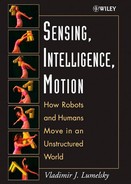
This procedure is executed at every point of the MA's (continuous) path [17, 58]. Before describing it formally, consider the behavior of MA when operating under this procedure (Figure 3.2). According to the definitions above, when on its way from point S (Start) to point T (Target), MA encounters an ith obstacle, it defines on it a hit point Hi,i = 1, 2,…. When leaving the ith obstacle in order to continue toward T, MA defines a leave point Li. Initially i = 1, L0 = S. The procedure will use three registers—R1, R2, and R3—to store intermediate information. All three are reset to zero when a new hit point is defined. The use of the registers is as follows:
- R1 is used to store coordinates of the latest point, Qm, of the minimum distance between the obstacle boundary and point T; this takes one comparison at each path point. (In case of many choices for Qm, any one of them can be taken.)
- R2 integrates the length of the ith obstacle boundary starting at Hi.
- R3 integrates the length of the ith obstacle boundary starting at Qm.
We are now ready to describe the algorithm's procedure. The test for target reachability mentioned in Step 3 of the procedure will be explained further in this section.
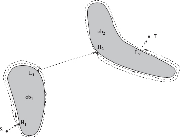
Figure 3.2 The path of the robot (dashed lines) under algorithm Bug1. ob1 and ob2 are obstacles, H1 and H2 are hit points, L1 and L2 are leave points.
Bug1 Procedure
- From point Li−1, move toward point T (Target) along the straight line until one of these occurs:
(a) Point T is reached. The procedure stops.
(b) An obstacle is encountered and a hit point, Hi, is defined. Go to Step 2.
- Using the local direction, follow the obstacle boundary. If point T is reached, stop. Otherwise, after having traversed the whole boundary and having returned to Hi, define a new leave point Li = Qm. Go to Step 3.
- Based on the contents of registers R2 and R3, determine the shorter way along the boundary to point Li, and use it to reach Li. Apply the test for target reachability. If point T is not reachable, the procedure stops. Otherwise, set i = i + 1 and go to Step 1.
Analysis of Algorithm Bug1
Lemma 3.3.1. Under Bug1 algorithm, when MA leaves a leave point of an obstacle in order to continue toward point T, it will never return to this obstacle again.
Proof: Assume that on its way from point S to point T, MA does meet some obstacles. We number those obstacles in the order in which MA encounters them. Then the following sequence of distances appears:
![]()
If point S happens to be on an obstacle boundary and the line (S, T) crosses that obstacle, then D = d(H1).
According to our model, if MA's path touches an obstacle tangentially, then MA needs not walk around it; it will simply continue its straight-line walk toward point T. In all other cases of meeting an ith obstacle, unless point T lies on an obstacle boundary, a relation d(Hi) > d(Li) holds. This is because, on the one hand, according to the model, any straight line (except a line that touches the obstacle tangentially) crosses the obstacle at least in two distinct points. This is simply a reflection of the finite “thickness” of obstacles. On the other hand, according to algorithm Bug1, point Li is the closest point from obstacle i to point T. Starting from Li, MA walks straight to point T until (if ever) it meets the (i + 1)th obstacle. Since, by the model, obstacles do not touch one another, then d(Li) > d(Hi+1). Our sequence of distances, therefore, satisfies the relation
where d(H1) is or is not equal to D. Since d(Li) is the shortest distance from the ith obstacle to point T, and since (3.6) guarantees that algorithm Bug1 monotonically decreases the distances d(Hi) and d(Li) to point T, Lemma 3.3.1 follows. Q.E.D.
The important conclusion from Lemma 3.3.1 is that algorithm Bug1 guarantees to never create cycles.
Corollary 3.3.1. Under Bug1, independent of the geometry of an obstacle, MA defines on it no more than one hit and no more than one leave point.
To assess the algorithm's performance—in particular, we will be interested in the upper bound on the length of paths that it generates—an assurance is needed that on its way to point T, MA can encounter only a finite number of obstacles. This is not obvious: While following the algorithm, MA may be “looking” at the target not only from different distances but also from different directions. That is, besides moving toward point T, it may also rotate around it (see Figure 3.3). Depending on the scene, this rotation may go first, say, clockwise, then counterclockwise, then again clockwise, and so on. Hence we have the following lemma.
Lemma 3.3.2. Under Bug1, on its way to the Target, MA can meet only a finite number of obstacles.
Proof: Although, while walking around an obstacle, MA may sometimes be at distances much larger than D from point T (see Figure 3.3), the straight-line segments of its path toward the point T are always within the same circle of radius D centered at point T. This is guaranteed by inequality (3.6). Since, according to our model, any disc of finite radius can intersect only a finite number of obstacles, the lemma follows. Q.E.D.
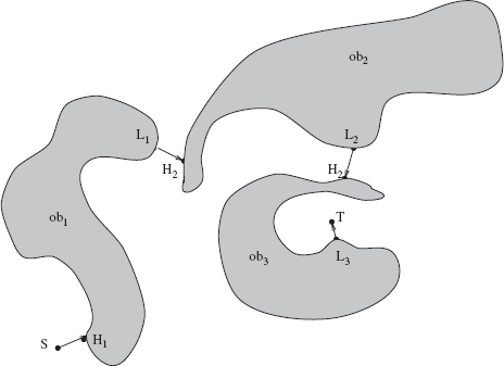
Figure 3.3 Algorithm Bug1. Arrows indicate straight-line segments of the robot's path. Path segments around obstacles are not shown; they are similar to those in Figure 3.2.
Corollary 3.3.2. The only obstacles that MA can be meet under algorithm Bug1 are those that intersect the disk of radius D centered at target T.
Together, Lemma 3.3.1, Lemma 3.3.2, and Corollary 3.3.2 guarantee convergence of the algorithm Bug1.
Theorem 3.3.1. Algorithm Bug1 is convergent.
We are now ready to tackle the performance of algorithm Bug1. As discussed, it will be established in terms of the length of paths that the algorithm generates. The following theorem gives an upper bound on the path lengths produced by Bug1.
Theorem 3.3.2. The length of paths produced by algorithm Bug1 obeys the limit,
where D is the distance (Start, Target), and Σi pi includes perimeters of obstacles intersecting the disk of radius D centered at the Target.
Proof: Any path generated by algorithm Bug1 can be looked at as consisting of two parts: (a) straight-line segments of the path while walking in free space between obstacles and (b) path segments when walking around obstacles. Due to inequality (3.6), the sum of the straight-line segments will never exceed D. As to path segments around obstacles, algorithm Bug1 requires that in order to define a leave point on the ith obstacle, MA has to first make a “full circle” along its boundary. This produces a path segment equal to one perimeter, pi, of the ith obstacle, with its end at the hit point. By the time MA has completed this circle and is ready to walk again around the ith obstacles from the hit to the leave point, in order to then depart for point T, the procedure prescribes it to go along the shortest path. By then, MA knows the direction (going left or going right) of the shorter path to the leave point. Therefore, its path segment between the hit and leave points along the ith obstacle boundary will not exceed 0.5 · pi. Summing up the estimates for straight-line segments of the path and segments around the obstacles met by MA on its way to point T, obtain (3.7). Q.E.D.
Further analysis of algorithm Bug1 shows that our model's requirement that MA knows its own coordinates at all times can be eased. It suffices if MA knows only its distance to and direction toward the target T. This information would allow it to position itself at the circle of a given radius centered at T. Assume that instead of coordinates of the current point Qm of minimum distance between the obstacle and T, we store in register R1 the minimum distance itself. Then in Step 3 of the algorithm, MA can reach point Qm by comparing its current distance to the target with the content of register R1. If more than one point of the current obstacle lie at the minimum distance from point T, any one of them can be used as the leave point, without affecting the algorithm's convergence.
In practice, this reformulated requirement may widen the variety of sensors the robot can use. For example, if the target sends out, equally in all directions, a low-frequency radio signal, a radio detector on the robot can (a) determine the direction on the target as one from which the signal is maximum and (b) determine the distance to it from the signal amplitude.
Test for Target Reachability. The test for target reachability used in algorithm Big1 is designed as follows. Every time MA completes its exploration of a new obstacle i, it defines on it a leave point Li. Then MA leaves the ith obstacle at Li and starts toward the target T along the straight line (Li, T). According to Lemma 3.3.1, MA will never return again to the ith obstacle. Since point Li is by definition the closest point of obstacle i to point T, there will be no parts of the obstacle i between points Li and T. Because, by the model, obstacles do not touch each other, point Li cannot belong to any other obstacle but i. Therefore, if, after having arrived at Li in Step 3 of the algorithm, MA discovers that the straight line (Li, T) crosses some obstacle at the leave point Li, this can only mean that this is the ith obstacle and hence target T is not reachable—either point S or point T is trapped inside the ith obstacle.
To show that this is true, let O be a simple closed curve; let X be some point in the scene that does not belong to O; let L be the point on O closest to X; and let (L, X) be the straight-line segment connecting L and X. All these are in the plane. Segment (L, X) is said to be directed outward if a finite part of it in the vicinity of point L is located outside of curve O. Otherwise, if segment (L, X) penetrates inside the curve O in the vicinity of L, it is said to be directed inward.
The following statement holds: If segment (L, X) is directed inward, then X is inside curve O. This condition is necessary because if X were outside curve O, then some other point of O that would be closer to X than to L would appear in the intersection of (L, X) and O. By definition of the point L, this is impossible. The condition is also sufficient because if segment (L, X) is directed inward and L is the point on curve O that is the closest to X, then segment (L, X) cannot cross any other point of O, and therefore X must lie inside O. This fact is used in the following test that appears as a part in Step 3 of algorithm Bug1:
Test for Target Reachability. If, while using algorithm Bug1, after having defined a point L on an obstacle, MA discovers that the straight line segment (L, Target) crosses the obstacle at point L, then the target is not reachable.
One can check the test on the example shown in Figure 3.4. Starting at point T, the robot encounters an obstacle and establishes on it a hit point H. Using the local direction “left,” it then does a full exploration of the (accessible) boundary of the obstacle. Once it arrives back at point H, its register R1 will contain the location of the point on the boundary that is the closest to T. This happens to be point L. The robot then walks to L by the shortest route (which it knows from the information it now has) and establishes on it the leave point L. At this point, algorithm Bug1 prescribes it to move toward T. While performing the test for target reachability, however, the robot will note that the line (L, T) enters the obstacle at L and hence will conclude that the target is not reachable.
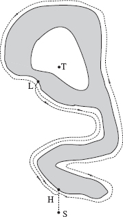
Figure 3.4 Algorithm Bug1. An example with an unreachable target (a trap).
3.3.2 Second Basic Algorithm: Bug2
Similar to the algorithm Bug1, the procedure Bug2 is executed at every point of the robot's (continuous) path. As before, the goal is to generate a path from the start to the target position. As will be evident later, three important properties distinguish algorithm Bug2 from Bug1: Under Bug2, (a) MA can encounter the same obstacle more than once, (b) algorithm Bug2 has no way of distinguishing between different obstacles, and (c) the straight line (S, T) that connects the starting and target points plays a crucial role in the algorithm's workings. The latter line is called M-line (for Main line). In imprecise words, the reason M-line is so important is that the procedure uses it to index its progress toward the target and to ensure that the robot does not get lost.
Because of these differences, we need to change the notation slightly: Subscript i will be used only when referring to more than one obstacle, and superscript j will be used to indicate the jth occurrence of a hit or leave points on the same or on a different obstacle. Initially, j = 1; L0 = Start. Similar to Bug1, the Bug2 procedure includes a test for target reachability, which is built into Steps 2b and 2c of the procedure. The test is explained later in this section. The reader may find it helpful to follow the procedure using an example in Figure 3.5.
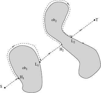
Figure 3.5 Robot's path (dashed line) under Algorithm Bug2.
- From point Lj−1, move along the M-line (straight line (S, T)) until one of these occurs:
(a) Target T is reached. The procedure stops.
(b) An obstacle is encountered and a hit point, Hj, is defined. Go to Step 2.
- Using the accepted local direction, follow the obstacle boundary until one of these occurs:
(a) Target T is reached. The procedure stops.
(b) M-line is met at a point Q such that distance d(Q) < d(Hj), and straight line (Q, T) does not cross the current obstacle at point Q. Define the leave point Lj = Q. Set j = j + 1. Go to Step 1.
(c) MA returns to Hj and thus completes a closed curve along the obstacle boundary, without having defined the next hit point, Hj+1. Then, the target point T is trapped and cannot be reached. The procedure stops.
Unlike with algorithm Bug1, more than one hit and more than one leave point can be generated on a single obstacle under algorithm Bug2 (see the example in Figure 3.6). Note also that the relationship between perimeters of the obstacles and the length of paths generated by Bug2 is not as clear as in the case of algorithm Bug1. In Bug1, the perimeter of an obstacle met by MA is traversed at least once and never more than l.5 times. In Bug2, more options appear. A path segment around an obstacle generated by MA is sometimes shorter than the obstacle perimeter (Figure 3.5), which is good news: We finally see something “intelligent.” Or, when a straight-line path segment of the path meets an obstacle almost tangentially and MA happened to be walking around the obstacle in an “unfortunate” direction, the path can become equal to the obstacle's full perimeter (Figure 3.7). Finally, as Figure 3.6a demonstrates, the situation can get even worse: MA may have to pass along some segments of a maze-like obstacle more than once and more than twice. (We will return to this case later in this section.)
Analysis of Algorithm Bug2
Lemma 3.3.3. Under Bug2, on its way to the target, MA can meet only a finite number of obstacles.
Proof: Although, while walking around an obstacle, MA may at times find itself at distances much larger than D from point T (Target), its straight-line path segments toward T are always within the same circle of radius D centered at T. This is guaranteed by the algorithm's condition that d(Lj, T) > d(Hj, T) (see Step 2 of Bug2 procedure). Since, by the model, any disc of finite radius can intersect with only a finite number of obstacles, the lemma follows. Q.E.D.
Corollary 3.3.3. The only obstacles that MA can meet while operating under algorithm Bug2 are those that intersect the disc of radius D centered at the target.

Figure 3.6 (a, b) Robot's path around a maze-like obstacle under Algorithm Bug2 (in-position case). Both obstacles (a) and (b) are similar, except in (a) the M-line (straight line (S, T)) crosses the obstacle 10 times, and in (b) it crosses 14 times. MA passes through the same path segment(s) at most three times (here, through segment (H1, L1)). Thus, at most two local cycles are created in this examples.
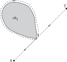
Figure 3.7 In this example, under Algorithm Bug2 the robot will make almost a full circle around this convex obstacle.

Figure 3.8 Robot's path in an in-position case; here point S is outside of the obstacle, and T is inside.
Moreover, the only obstacles that can be met by MA are those that intersect the M-line (straight line (Start, Target)).
Definition 3.3.1. For the given local direction, a local cycle is created when MA has to pass some point of its path more than once.
In the example in Figure 3.5, no local cycles are created; in Figures 3.6 and 3.8 there are local cycles.
Definition 3.3.2. The term in-position refers to a mutual position of points (Start, Target) and a given obstacle, such that (1) the M-line crosses the obstacle boundary at least once, and (2) either Start or Target lie inside the convex hull of the obstacle. The term out-position refers to a mutual position of points (Start, Target) and a given obstacle, such that both points Start and Target lie outside the convex hull of the obstacle. A given scene is referred to as an in-position case if at least one obstacle in the scene creates an in-position situation; otherwise, the scene presents an out-position case.
For example, the scene in Figure 3.3 is an in-position case. Without obstacle ob3, the scene would have been an out-position case.
We denote ni to be the number of intersections between the M-line (straight line (S, T)) and the ith obstacle; ni is thus a characteristic of the set (scene, Start, Target) and not of the algorithm. Obviously, for any convex obstacle, ni = 2.
If an obstacle is not convex but still ni = 2, the path generated by Bug2 can be as simple as that for a convex obstacle (see, e.g., Figure 3.5, obstacle ob2). Even with more complex obstacles, such as that in Figure 3.6, the situation and the resulting path can be quite simple. For example, in this same scene, if the M-line happened to be horizontal, we would have ni = 2 and a very simple path.
The path can become more complicated if ni > 2 and we are dealing with an in-position case. In Figure 3.6a, the segment of the boundary from point H1 to point L1, (H1, L1), will be traversed three times: segments (L1, L2) and (H2, H1), twice each; and segments (L2, L3) and (H3, H2), once each. On the other hand, if in this example the M-line line extends below, so that point S is under the whole obstacle (that is, this becomes an out-position case), the path will again become very simple, with no local cycles (in spite of high ni number).
Lemma 3.3.4. Under Bug2, MA will pass any point of the ith obstacle boundary at most ni/2 times.
Proof: As one can see, procedure Bug2 does not distinguish whether two consecutive obstacle crossings by the M-line (straight line (S, T)) correspond to the same or to different obstacles. Without loss of generality, assume that only one obstacle is present; then we can drop the index i. For each hit point Hj, the procedure will make MA walk around the obstacle until it reaches the corresponding leave point, Lj. Therefore, all H and L points appear in pairs, (Hj, Lj). Because, by the model, all obstacles are of finite “thickness,” for each pair (Hj, Lj) an inequality holds, d(Hj) > d(Lj). After leaving Lj, MA walks along a straight line to the next hit point, Hj+1. Since, according to the model, the distance between two crossings of the obstacle by a straight line is finite, we have d(Lj) > d(Hj+1). This produces a chain of inequalities for all H and L points,
Therefore, although any H or L point may be passed more than once, it will be defined as an H(correspondingly, L) point only once. That point can hence generate only one new passing of the same segment of the obstacle perimeter. In other words, each pair (Hj, Lj) can give rise to only one passing of a segment of the obstacle boundary. This means that ni crossings will produce at most ni/2 passings of the same path segment. Q.E.D.
The lemma guarantees that the procedure terminates, and it gives a limit on the number of generated local cycles. Using the lemma, we can now produce an upper bound on the length of paths generated by algorithm Bug2.
Theorem 3.3.3. The length of a path generated by algorithm Bug2 will never exceed the limit
where D is the distance (Start, Target), and pi refers to perimeters of obstacles that intersect the M-line (straight line segment (Start, Target)). This means Bug2 is convergent.
Proof: Any path can be looked at as consisting of two parts: (a) straight-line segments of the M-line between the obstacles that intersect it and (b) path segments that relate to walking around obstacle boundaries. Because of inequality (3.8), the sum of the straight line segments will never exceed D. As to path segments around obstacles, there is an upper bound guaranteed by Lemma 3.3.4 for each obstacle met by MA on its path: No more than ni/2 passings along the same segment of the obstacle boundary will take place. Because of Lemma 3.3.3 (see its proof), only those obstacles that intersect the M-line should be counted. Summing up the straight-line segments and segments that correspond to walking around obstacles, obtain (3.9). Q.E.D.
Theorem 3.3.3 suggests that in some “bad” scenes, under algorithm Bug2, MA may be forced to go around obstacles any large, albeit finite, number of times. An important question, therefore, is how typical such “bad” scenes are.
In particular, other things being equal, what characteristics of the scene influence the length of the path? Theorem 3.3.4 and its corollary below address this question. They suggest that the mutual position of point S, point T, and obstacles in the scene can affect the path length rather dramatically. Together, they significantly improve the upper bound on the length of paths generated by Bug2—in out-position scenes in general and in scenes with convex obstacles in particular.
Theorem 3.3.4. Under algorithm Bug2, in the case of an out-position scene, MA will pass any point of an obstacle boundary at most once.
In other words, if the mutual position of the obstacle and of points S and T satisfies the out-position definition, the estimate on the length of paths generated by Bug2 reaches the universal lower bound (3.1). That is a very good news indeed. Out-position situations are rather common for mobile robots.3 We know already that in some situations, algorithm Bug2 is extremely efficient and traverses only a fraction of obstacle boundaries. Now the theorem tells us that as long as the robot deals with an out-position situation, even in the most unlucky case it will not traverse more than 1.5 times the obstacle boundaries involved.
Proof: Figure 3.9 is used to illustrate the proof. Shaded areas in the figure correspond to one or many obstacles. Dashed boundaries indicate that obstacle boundaries in these areas can be of any shape.
Consider an obstacle met by MA on its way to the Target, and consider an arbitrary point Q on the obstacle boundary (not shown in the figure). Assume that Q is not a hit point. Because the obstacle boundary is a simple closed curve, the only way that MA can reach point Q is to come to it from a previously defined hit point. Now, move from Q along the already generated path segment in the direction opposite to the accepted local direction, until the closest hit point on the path is encountered; say, that point is Hj. We are interested only in those cases where Q is involved in at least one local cycle—that is, when MA passes point Q more than once. For this event to occur, MA has to pass point Hj at least as many times. In other words, if MA does not pass Hj more than once, it cannot pass Q more than once.

Figure 3.9 Illustration for Theorem 3.3.4.
According to the Bug2 procedure, the first time MA reaches point Hj it approaches it along the M-line (straight line (Start, Target))—or, more precisely, along the straight line segment (Lj−1, T). MA then turns left and starts walking around the obstacle. To form a local cycle on this path segment, MA has to return to point Hj again. Since a point can become a hit point only once (see the proof for Lemma 3.3.4), the next time MA returns to point Hj it must approach it from the right (see Figure 3.9), along the obstacle boundary. Therefore, after having defined Hj, in order to reach it again, this time from the right, MA must somehow cross the M-line and enter its right semiplane. This can take place in one of only two ways: outside or inside the interval (S, T). Consider both cases.
- The crossing occurs outside the interval (S, T). This case can correspond only to an in-position configuration (see Definition 3.3.2). Theorem 3.3.4, therefore, does not apply.
- The crossing occurs inside the interval (S, T). We want to prove now that such a crossing of the path with the interval (S, T) cannot produce local cycles. Notice that the crossing cannot occur anywhere within the interval (S, H j) because otherwise at least a part of the straight-line segment (Lj−1, Hj) would be included inside the obstacle. This is impossible because MA is known to have walked along the whole segment (Lj−1, Hj). If the crossing occurs within the interval (Hj, T), then at the crossing point MA would define the corresponding leave point, Lj, and start moving along the line (S, T) toward the target T until it defined the next hit point, Hj+1, or reached the target. Therefore, between points Hj and Lj, MA could not have reached into the right semiplane of the M-line (see Figure 3.9).
Since the above argument holds for any Q and the corresponding Hj, we conclude that in an out-position case MA will never cross the interval (Start, Target) into the right semiplane, which prevents it from producing local cycles. Q.E.D.
So far, no constraints on the shape of the obstacles have been imposed. In a special case when all the obstacles in the scene are convex, no in-position configurations can appear, and the upper bound on the length of paths generated by Bug2 can be improved:
Corollary 3.3.4. If all obstacles in the scene are convex, then in the worst case the length of the path produced by algorithm Bug2 is
and, on the average,
where D is distance (Start, Target), and pi refer to perimeters of the obstacles that intersect the straight line segment (Start, Target).
Consider a statistically representative number of scenes with a random distribution of convex obstacles in each scene, a random distribution of points Start and Target over the set of scenes, and a fixed local direction as defined above. The M-line will cross obstacles that it intersects in many different ways. Then, for some obstacles, MA will be forced to cover the bigger part of their perimeters (as in the case of obstacle ob1, Figure 3.5); for some other obstacles, MA will cover only a smaller part of their perimeters (as with obstacle ob2, Figure 3.5).
On the average, one would expect a path that satisfies (3.11). As for (3.10), Figure 3.7 presents an example of such a “noncooperating” obstacle. Corollary 3.3.4 thus ensures that for a wide range of scenes the length of paths generated by algorithm Bug2 will not exceed the universal lower bound (3.1).
Test for Target Reachability. As suggested by Lemma 3.3.4, under Bug2 MA may pass the same point Hj of a given obstacle more than once, producing a finite number p of local cycles, p = 0, 1, 2,…. The proof of the lemma indicates that after having defined a point Hj, MA will never define this point again as an H or an L point. Therefore, on each of the subsequent local cycles (if any), point Hj will be passed not along the M-line but along the obstacle boundary. After having left point Hj, MA can expect one of the following to occur:
MA will never return again to Hj; this happens, for example, if it leaves the current obstacle altogether or reaches the Target T.
MA will define at least the first pair of points (Lj, Hj+1), … , and will then return to point Hj, to start a new local cycle.
MA will come back to point Hj without having defined a point Lj on the previous cycle. This means that MA could find no other intersection point Q of the line (Hj, T) with the current obstacle such that Q would be closer to the point T than Hj, and the line (Q, T) would not cross the current obstacle at Q. This can happen only if either MA or point T are trapped inside the current obstacle (see Figure 3.10). The condition is both necessary and sufficient, which can be shown similar to the proof in the target reachability test for algorithm Bug1 (Section 3.3.1).
Based on this observation, we now formulate the test for target reachability for algorithm Bug2.

Figure 3.10 Examples where no path between points S and T is possible (traps), algorithm Bug2. The path is the dashed line. After having defined the hit point H2, the robot returns to it before it defines any new leave point. Therefore, the target is not reachable.
Test for Target Reachability. If, on the pth local cycle, p = 0, 1, … , after having defined a hit point Hj, MA returns to this point before it defines at least the first two out of the possible set of points Lj, Hj+1, … , Hk, this means that MA has been trapped and hence the target is not reachable.
We have learned that in in-position situations algorithm Bug2 may become inefficient and create local cycles, visiting some areas of its path more than once. How can we characterize those situations? Does starting or ending “inside” the obstacle—that is, having an in-position situation—necessarily lead to such inefficiency? This is clearly not so, as one can see from the following example of Bug2 operating in a maze (labyrinth). Consider a version of the labyrinth problem where the robot, starting at one point inside the labyrinth, must reach some other point inside the labyrinth. The well-known mice-in-the-labyrinth problem is sometimes formulated this way. Consider an example4 shown in Figure 3.11.

Figure 3.11 Example of a walk (dashed line) in a maze under algorithm Bug2. S, Start; T, Target.
Given the fact that no bird's-eye view of the maze is available to MA (at each moment it can see only the small cell that it is passing), the MA's path looks remarkably efficient and purposeful. (It would look even better if MA's sensing was something better than simple tactile sensing; see Figure 3.20 and more on this topic in Section 3.6.) One reason for this is, of course, that no local cycles are produced here. In spite of its seeming complexity, this maze is actually an easy scene for the Bug2 algorithm.
Let's return to our question, How can we classify in-position situations, so as to recognize which one would cause troubles to the algorithm Bug2? This question is not clear at the present time. The answer, likely tied to the topological properties of the combination (scene, Start, Target), is still awaiting a probing researcher.
3.4 COMBINING GOOD FEATURES OF BASIC ALGORITHMS
Each of the algorithms Bug1 and Bug2 has a clear and simple, and quite distinct, underlying idea: Bug1 “sticks” to every obstacle it meets until it explores it fully; Bug2 sticks to the M-line (line (Start, Target)). Each has its pluses and minuses. Algorithm Bug1 never creates local cycles; its worse-case performance looks remarkably good, but it tends to be “overcautious” and will never cover less than the full perimeter of an obstacle on its way. Algorithm Bug2, on the other hand, is more “human” in that it can “take a risk.” It takes advantage of simpler situations; it can do quite well even in complex scenes in spite of its frighteningly high worst-case performance—but it may become quite inefficient, much more so than Bug1, in some “unlucky” cases.
The difficulties that algorithm Bug2 may face are tied to local cycles— situations when the robot must make circles, visiting the same points of the obstacle boundaries more than once. The source of these difficulties lies in what we called in-position situations (see the Bug2 analysis above). The problem is of topological nature. As the above estimates of Bug2 “average” behavior show, its performance in out-positions situations may be remarkably good; these are situations that mobile robots will likely encounter in real-life scenes.
On the other hand, fixing the procedure so as to handle in-position situations well would be an important improvement. One simple idea for doing this is to attempt a procedure that combines the better features of both basic algorithms. (As always, when attempting to combine very distinct ideas, the punishment will be the loss of simplicity and elegance of both algorithms.) We will call this procedure BugM1 (for “modified”) [59]. The procedure combines the efficiency of algorithm Bug2 in simpler scenes (where MA will pass only portions, instead of full perimeters, of obstacles, as in Figure 3.5) with the more conservative, but in the limit the more economical, strategy of algorithm Bug1 (see the bound (3.7)). The idea is simple: Since Bug2 is quite good except in cases with local cycles, let us try to switch to Bug1 whenever MA concludes that it is in a local cycle. As a result, for a given point on a BugM1 path, the number of local cycles containing this point will never be larger than two; in other words, MA will never pass the same point of the obstacle boundary more than three times, producing the upper bound
Algorithm BugM1 is executed at every point of the continuous path. Instead of using the fixed M-line (straight line (S, T)), as in Bug2, BugM1 uses a straight-line segment ![]() with a changing point
with a changing point ![]() here,
here, ![]() indicates the jth leave point on obstacle i. The procedure uses three registers, R1, R2, and R3, to store intermediate information. All three are reset to zero when a new hit point
indicates the jth leave point on obstacle i. The procedure uses three registers, R1, R2, and R3, to store intermediate information. All three are reset to zero when a new hit point ![]() is defined:
is defined:
- Register R1 stores coordinates of the current point, Qm, of minimum distance between the obstacle boundary and the Target.
- R2 integrates the length of the obstacle boundary starting at
 .
. - R3 integrates the length of the obstacle boundary starting at Qm. (In case of many choices for Qm, any one of them can be taken.)
The test for target reachability that appears in Step 2d of the procedure is explained lower in this section. Initially, i = 1, j = 1; ![]() = Start. The BugM1 procedure includes these steps:
= Start. The BugM1 procedure includes these steps:
- From point
 , move along the line (
 , Target) toward Target until one of these occurs:
(a) Target is reached. The procedure stops.
(b) An ith obstacle is encountered and a hit point,
, is defined. Go to Step 2. - Using the accepted local direction, follow the obstacle boundary until one of these occurs:
(a) Target is reached. The procedure stops.
(b) Line (
, Target) is met inside the interval (, Target), at a point Q such that distance d(Q) < d(Hj), and the line (Q, Target) does not cross the current obstacle at point Q. Define the leave point  = Q. Set j = j + 1. Go to Step 1.
(c) Line (
, Target) is met outside the interval (, Target). Go to Step 3.(d) The robot returns to
and thus completes a closed curve (of the obstacle boundary) without having defined the next hit point. The target cannot be reached. The procedure stops. - Continue following the obstacle boundary. If the target is reached, stop. Otherwise, after having traversed the whole boundary and having returned to point , define a new leave point
 . Go to Step 4.
 - Using the contents of registers R2 and R3, determine the shorter way along the obstacle boundary to point , and use it to get to . Apply the test for Target reachability (see below). If the target is not reachable, the procedure stops. Otherwise, designate
 , set i = i + 1, j = 1, and go to Step 1.
As mentioned above, the procedure itself BugM1 is obviously longer and “messier” compared to the elegantly simple procedures Bug1 and Bug2. That is the price for combining two algorithms governed by very different principles. Note also that since at times BugM1 may leave an obstacle before it fully explores it, according to our classification above it falls into the Class 2.
What is the mechanism of algorithm BugM1 convergence? Depending on the scene, the algorithm's flow fits one of the following two cases.
Case 1. If the condition in Step 2c of the procedure is never satisfied, then the algorithm flow follows that of Bug2—for which convergence has been already established. In this case, the straight lines (![]() , Target) always coincide with the M-line (straight line (Start, Target)), and no local cycles appear.
, Target) always coincide with the M-line (straight line (Start, Target)), and no local cycles appear.
Case 2. If, on the other hand, the scene presents an in-position case, then the condition in Step 2c is satisfied at least once; that is, MA crosses the straight line (![]() , Target) outside the interval (
, Target) outside the interval (![]() , Target). This indicates that there is a danger of multiple local cycles, and so MA switches to a more conservative procedure Bug1, instead of risking an uncertain number of local cycles it might now expect from the procedure Bug2 (see Lemma 3.3.4). MA does this by executing Steps 3 and 4 of BugM1, which are identical to Steps 2 and 3 of Bug1.
, Target). This indicates that there is a danger of multiple local cycles, and so MA switches to a more conservative procedure Bug1, instead of risking an uncertain number of local cycles it might now expect from the procedure Bug2 (see Lemma 3.3.4). MA does this by executing Steps 3 and 4 of BugM1, which are identical to Steps 2 and 3 of Bug1.
After one execution of Steps 3 and 4 of the BugM1 procedure, the last leave point on the ith obstacle is defined, ![]() , which is guaranteed to be closer to point T than the corresponding hit point,
, which is guaranteed to be closer to point T than the corresponding hit point, ![]() [see inequality (3.7), Lemma 3.3.1]. Then MA leaves the ith obstacle, never to return to it again (Lemma 3.3.1). From now on, the algorithm (in its Steps 1 and 2) will be using the straight line (
[see inequality (3.7), Lemma 3.3.1]. Then MA leaves the ith obstacle, never to return to it again (Lemma 3.3.1). From now on, the algorithm (in its Steps 1 and 2) will be using the straight line (![]() , Target) as the “leading thread.” [Note that, in general, the line (
, Target) as the “leading thread.” [Note that, in general, the line (![]() , Target) does not coincide with the straight lines (
, Target) does not coincide with the straight lines (![]() , T) or (S, T)]. One execution of the sequence of Steps 3 and 4 of BugM1 is equivalent to one execution of Steps 2 and 3 of Bug1, which guarantees the reduction by one of the number of obstacles that MA will meet on its way. Therefore, as in Bug1, the convergence of this case is guaranteed by Lemma 3.3.1, Lemma 3.3.2, and Corollary 3.3.2. Since Case 1 and Case 2 above are independent and together exhaust all possible cases, the procedure BugM1 converges.
, T) or (S, T)]. One execution of the sequence of Steps 3 and 4 of BugM1 is equivalent to one execution of Steps 2 and 3 of Bug1, which guarantees the reduction by one of the number of obstacles that MA will meet on its way. Therefore, as in Bug1, the convergence of this case is guaranteed by Lemma 3.3.1, Lemma 3.3.2, and Corollary 3.3.2. Since Case 1 and Case 2 above are independent and together exhaust all possible cases, the procedure BugM1 converges.
3.5 GOING AFTER TIGHTER BOUNDS
The above analysis raises two questions:
- There is a gap between the bound given by (3.1), P > D + Σi pi − δ (the universal lower bound for the planning problem), and the bound given by (3.7), P < D + 1.5 · Σi pi (the upper bound for Bug1 algorithm).
What is there in the gap? Can the lower bound (3.1) be tightened upwards—or, inversely, are there algorithms that can reach it?
- How big and diverse are Classes 1 and 2?
To remind the reader, Class 1 combines algorithms in which the robot never leaves an obstacle unless and until it explores it completely. Class 2 combines algorithms that are complementary to those in Class 1: In them the robot can leave an obstacle and walk further, and even return to this obstacle again at some future time, without exploring it in full.
A decisive step toward answering the above questions was made in 1991 by A. Sankaranarayanan and M. Vidyasagar [60]. They proposed to (a) analyze the complexity of Classes 1 and 2 of sensor-based planning algorithms separately and (b) obtain the lower bounds on the lengths of generated paths for each of them. This promised tighter bounds compared to (3.1). Then, since together both classes cover all possible algorithms, the lower of the obtained bounds would become the universal lower bound. Proceeding in this direction, Sankaranarayanan and Vidyasagar obtained the lower bound for Class 1 algorithms as
and the lower bound for Class 2 algorithms as
As before, P is the length of a generated path, D is the distance (Start, Target), and pi refers to perimeters of obstacles met by the robot on its way to the target.
There are three important conclusions from these results:
- It is the bound (3.13), and not (3.1), that is today the universal lower bound: in the worst case no sensor-based motion planning algorithm can produce a path shorter than P in (3.13).
- According to the bound (3.13), algorithm Bug1 reaches the universal lower bound. That is, no algorithm in Class 1 will be able to do better than Bug1 in the worst case.
- According to bounds (3.13) and (3.14), in the worst case no algorithm from either of the two classes can do better than Bug1.
How much variety and how many algorithms are there in Classes 1 and 2? For Class 1, the answer is simple: At this time, algorithm Bug1 is the only representative of Class 1. The future will tell whether this represents just the lack of interest in the research community to such algorithms or something else. One can surmise that it is both: The underlying mechanism of this class of algorithms does not promise much richness or unusual algorithms, and this gives little incentive for active research.
In contrast, a lively innovation and variety has characterized the development in Class 2 algorithms. At least a dozen or so algorithms have appeared in literature since the problem was first formulated and the basic algorithms were reported. Since some such algorithms make use of the types of sensing that are more elaborate than basic tactile sensing used in this section, we defer a survey in this area until Section 3.8, after we discuss in the next section the effect of more complex sensing on sensor-based motion planning.
3.6 VISION AND MOTION PLANNING
In the previous section we developed the framework for designing sensor-based path planning algorithms with proven convergence. We designed some algorithms and studied their properties and performance. For clarity, we limited the sensing that the robot possesses to (the most simple) tactile sensing. While tactile sensing plays an important role in real-world robotics—in particular in short-range motion planning for object manipulation and for escaping from tight places—for general collision avoidance, richer remote sensing such as computer vision or range sensing present more promising options.
The term “range” here refers to devices that directly provide distance information, such as a laser ranger. A stereo vision device would be another option. In order to successfully negotiate a scene with obstacles, a mobile robot can make a good use of distance information to objects it is passing.
Here we are interested in exploring how path planning algorithms would be affected by the sensing input that is richer and more complex than tactile sensing. In particular, can algorithms that operate with richer sensory data take advantage of additional sensor information and deliver better path length performance—to put it simply, shorter paths—than when using tactile sensing? Does proximal or distant sensing really help in motion planning compared to tactile sensing, and, if so, in what way and under what conditions? Although this question is far from trivial and is important for both theory and practice (this is manifested by a recent continuous flow of experimental works with “seeing” robots), there have been little attempts to address this question on the algorithmic level.
We are thus interested in algorithms that can make use of a range finder or stereo vision and that, on the one hand, are provably correct and, on the other hand, would let, say, a mobile robot deliver a reasonable performance in nontrivial scenes. It turns out that the answers to the above question are not trivial as well. First, yes, algorithms can be modified so as to take advantage of better sensing. Second, extensive modifications of “tactile” motion planning algorithms are needed in order to fully utilize additional sensing capabilities. We will consider in detail two principles for provably correct motion planning with vision. As we will see, the resulting algorithms exhibit different “styles” of behavior and are not, in general, superior to each other. Third and very interestingly, while one can expect great improvements in real-world tasks, in general richer sensing has no effect on algorithm path length performance bounds.
Algorithms that we are about to consider will demonstrate an ability that is often referred to in the literature as active vision [61, 62]. This ability goes deeply into the nature of interaction between sensing and control. As experimentalists well know, scanning the scene and making sense of acquired information is a time-consuming operation. As a rule, the robot's “eye” sees a bewildering amount of details, almost all of which are irrelevant for the robot's goal of finding its way around. One needs a powerful mechanism that would reject what is irrelevant and immediately use what is relevant so that one can continue the motion and continue gathering more visual data. We humans, and of course all other species in nature that use vision, have such mechanisms.
As one will see in this section, motion planning algorithms with vision that we will develop will provide the robot with such mechanisms. As a rule, the robot will not scan the whole scene; it will behave much as a human when walking along the street, looking for relevant information and making decisions when the right information is gathered. While the process is continuous, for the sake of this discussion it helps to consider it as a quasi-discrete.
Consider a moment when the robot is about to pass some location. A moment earlier, the robot was at some prior location. It knows the direction toward the target location of its journey (or, sometimes, some intermediate target in the visible part of the scene). The first thing it does is look in that direction, to see if this brings new information about the scene that was not available at the prior position. Perhaps it will look in the direction of its target location. If it sees an obstacle in that direction, it may widen its “scan,” to see how it can pass around this obstacle. There may be some point on the obstacle that the robot will decide to head to, with the idea that more information may appear along the way and the plan may be modified accordingly.
Similar to how any of us behaves when walking, it makes no sense for the robot to do a 360° scan at every step—or ever. Based on what the robot sees ahead at any moment, it decides on the next step, executes it, and looks again for more information. In other words, robot's sensing dictates the next step motion, and the next step dictates where to look for new relevant information. It is this sensing-planning control loop that guides the robot's active vision, and it is executed continuously.
The first algorithm that we will consider, called VisBug-21, is a rather simple-minded and conservative procedure. (The number “2” in its name refers to the Bug2 algorithm that is used as its base, and “1” refers to the first vision algorithm.) It uses range data to “cut corners” that would have been produced by a “tactile” algorithm Bug2 operating in the same scene. The advantage of this modification is clear. Envision the behavior of two people, one with sight and the other blindfolded. Envision each of them walking in the same direction around the perimeter of a complex-shaped building. The path of the person with sight will be (at least, often enough) a shorter approximation of the path of the blindfolded person.
The second algorithm, called VisBug-22, is more opportunistic in nature: it tries to use every chance to get closer to the target. (The number in its name signifies that it is the vision algorithm 2 based on the Bug2 procedure.)
Section 3.6.1 is devoted to the algorithms' underlying model and basic ideas. The algorithms themselves, related analysis, and examples demonstrating the algorithms' performance appear in Sections 3.6.2 and 3.6.3.
3.6.1 The Model
Our assumptions about the scene in which the robot travels and about the robot itself are very much the same as for the basic algorithms (Section 3.1). The available input information includes knowing at all times the robot's current location, C, and the locations of starting and target points, S and T. We also assume that a very limited memory does not allow the robot more than remembering a few “interesting” points.
The difference in the two models relates to the robot sensing ability. In the case at hand the robot has a capability, referred to as vision, to detect an obstacle, and the distance to any visible point of it, along any direction from point C, within the sensor's field of vision. The field of vision presents a disc of radius rυ, called radius of vision, centered at C. A point Q in the scene is visible if it is located within the field of vision and if the straight-line segment CQ does not cross any obstacles.
The robot is capable of using its vision to scan its surroundings during which it identifies obstacles, or the lack of thereof, that intersect its field of vision. We will see that the robot will use this capability rather sparingly; the particular use of scanning will depend on the algorithm. Ideally the robot will scan a part of the scene only in those specific directions that make sense from the standpoint of motion planning. The robot may, for example, identify some intermediate target point within its field of vision and walk straight toward that point. Or, in an “unfortunate” (for its vision) case when the robot walks along the boundary of a convex obstacle, its effective radius of vision in the direction of intended motion (that is, around the obstacle) will shrink to zero.
As before, the straight-line segment (S, T) between the start S and target T points—it is called the Main line or M-line—is the desirable path. Given its current position Ci, at moment i the robot will execute an elementary operation that includes scanning some minimum sector of its current field of vision in the direction it is following, enough to define its next intermediate target, point Ti. Then the robot makes a little step in the direction of Ti, and the process repeats. Ti is thus a moving target; its choice will somehow relate to the robot's global goal. In the algorithms, every Ti will lie on the M-line or on an obstacle boundary.
For a path segment whose point Ti moves along the M-line, the firstly defined Ti that lies at the intersection of M-line and an obstacle is a special point called the hit point, H. Recall that in algorithms Bug1 or Bug2 a hit point would be reached physically. In algorithms with vision a hit point may be defined from a distance, thanks to the robot's vision, and the robot will not necessarily pass through this location. For a path segment whose point Ti moves along an obstacle boundary, the firstly defined Ti that lies on the M-line is a special point called the leave point, L. Again, the robot may or may not pass physically through that point. As we will see, the main difference between the two algorithms VisBug-21 and VisBug-22 is in how they define intermediate targets Ti. Their resulting paths will likely be quite different. Naturally, the current Ti is always at a distance from the robot no more than rυ.
While scanning its field of vision, the robot may be detecting some contiguous sets of visible points—for example, a segment of the obstacle boundary. A point Q is contiguous to another point S over the set {P}, if three conditions are met: (i) S ∈ {P}, (ii) Q and {P} are visible, and (iii) Q can be continuously connected with S using only points of {P}. A set is contiguous if any pair of its points are contiguous to each other over the set. We will see that no memorization of contiguous sets will be needed; that is, while “watching” a contiguous set, the robot's only concern will be whether two points that it is currently interested in are contiguous to each other.
A local direction is a once-and-for-all determined direction for passing around an obstacle; facing the obstacle, it can be either left or right. Because of incomplete information, neither local direction can be judged better than the other. For the sake of clarity, assume the local direction is always left.
The M-line divides the environment into two half-planes. The half-plane that lies to the local direction's side of M-line is called the main semiplane. The other half-plane is called the secondary semiplane. Thus, with the local direction “left,” the left half-plane when looking from S toward T is the main semiplane.
Figure 3.12 exemplifies the defined terms. Shaded areas represent obstacles; the straight-line segment ST is the M-line; the robot's current location, C, is in the secondary (right) semiplane; its field of vision is of radius rυ. If, while standing at C, the robot were to perform a complete scan, it would identify three contiguous segments of obstacle boundaries, a1a2a3, a4a5a6a7a8, and a9a10a11, and two contiguous segments of M-line, b1b2 and b3b4.
A Sketch of Algorithmic Ideas. To understand how vision sensing can be incorporated in the algorithms, consider first how the “pure” basic algorithm Bug2 would behave in the scene shown in Figure 3.12. Assuming a local direction “left,” Bug2 would generate the path shown in Figure 3.13. Intuitively, replacing tactile sensing with vision should smooth sharp corners in the path and perhaps allow the robot to cut corners in appropriate places.
However, because of concern for algorithms' convergence, we cannot introduce vision in a direct way. One intuitively appealing idea is, for example, to make the robot always walk toward the farthest visible “corner” of an obstacle in the robot's preferred direction. An example can be easily constructed showing that this idea cannot work—it will ruin the algorithm convergence. (We have already seen examples of treachery of intuitively appealing ideas; see Figure 2.23—it applies to the use of vision as well.)

Figure 3.12 Shaded areas are obstacles. At its current location C, the robot will see within its radius of vision rυ segments of obstacle boundaries a1a2a3, a4a5a6a7a8, and a9a10a11. It will also conclude that segments b1b2 and b3b4 of the M-line are visible.

Figure 3.13 Scene 1: Path generated by the algorithm Bug2.
Since algorithm Bug2 is known to converge, one way to incorporate vision is to instruct the robot at each step of its path to “mentally” reconstruct in its current field of vision the path segment that would have been produced by Bug2 (let us call it the Bug2 path). The farthest point of that segment can then be made the current intermediate target point, and the robot would make a step toward that point. And then the process repeats. To be meaningful, this would require an assurance of continuity of the considered Bug2 path segment; that is, unless we know for sure that every point of the segment is on the Bug2 path, we cannot take a risk of using this segment. Just knowing the fact of segment continuity is sufficient; there is no need to remember the segment itself. As it turns out, deciding whether a given point lies on the Bug2 path—in which case we will call it a Bug2 point —is not a trivial task. The resulting algorithm is called VisBug-21, and the path it generates is referred to as the VisBug-21 path.
The other algorithm, called VisBug-22, is also tied to the mechanism of Bug2 procedure, but more loosely. The algorithm behaves more opportunistically compared to VisBug-21. Instead of the VisBug-21 process of replacing some “mentally” reconstructed Bug2 path segments with straight-line shortcuts afforded by vision, under VisBug-22 the robot can deviate from Bug2 path segments if this looks more promising and if this is not in conflict with the convergence conditions. As we will see, this makes VisBug-22 a rather radical departure from the Bug2 procedure—with one result being that Bug2 cannot serve any longer as a source of convergence. Hence convergence conditions in VisBug-22 will have to be established independently.
In case one wonders why we are not interested here in producing a vision-laden algorithm extension for the Bug1 algorithm, it is because savings in path length similar to the VisBug-21 and VisBug-22 algorithms are less likely in this direction. Also, as mentioned above, exploring every obstacle completely does not present an attractive algorithm for mobile robot navigation.
Combining Bug1 with vision can be a viable idea in other motion planning tasks, though. One problem in computer vision is recognizing an object or finding a specific item on the object's surface. One may want, for example, to automatically detect a bar code on an item in a supermarket, by rotating the object to view it completely. Alternatively, depending on the object's dimensions, it may be the viewer who moves around the object. How do we plan this rotating motion? Holding the camera at some distance from the object gives the viewer some advantages. For example, since from a distance the camera will see a bigger part of the object, a smaller number of images will be needed to obtain the complete description of the object [63].
Given the same initial conditions, algorithms VisBug-21 and VisBug-22 will likely produce different paths in the same scene. Depending on the scene, one of them will produce a shorter path than the other, and this may reverse in the next scene. Both algorithms hence present viable options. Each algorithm includes a test for target reachability that can be traced to the Bug2 algorithm and is based on the following necessary and sufficient condition:
Test for Target Reachability. If, after having defined the last hit point as its intermediate target, the robot returns to it before it defines the next hit point, then either the robot or the target point is trapped and hence the target is not reachable. (For more detail, see the corresponding text for algorithm Bug2.)
The following notation is used in the rest of this section:
- Ci and Ti are the robot's position and intermediate target at step i.
- |AB| is the straight-line segment whose endpoints are A and B; it may also designate the length of this segment.
- (AB) is the obstacle boundary segment whose endpoints are A and B, or the length of this segment.
- [AB] is the path segment between points A and B that would be generated by algorithm Bug2, or the length of this path segment.
- {AB} is the path segment between points A and B that would be generated by algorithm VisBug-21 or VisBug-22, or the length of this path segment.
It will be evident from the context whether a given notation is referring to a segment or its length. When more than one segment appears between points A and B, the context will resolve the ambiguity.
3.6.2 Algorithm VisBug-21
The algorithm consists of the Main body, which does the motion planning proper, and a procedure called Compute Ti-21, which produces the next intermediate target Ti and includes the test for target reachability. As we will see, typically the flow of action in the main body is confined to its step S1. Step S2 is executed only in the special case when the robot is moving along a (locally) convex obstacle boundary and so it cannot use its vision to define the next intermediate target Ti. For reasons that will become clear later, the algorithm distinguishes between the case when point Ti lies in the main semiplane and the case when Ti lies in the secondary semiplane. Initially, C = Ti = S.
Main Body. The procedure is executed at each point of the continuous path. It includes the following steps:
- S1: Move toward point Ti while executing Compute Ti-21 and performing the following test:
If C = T the procedure stops.
Else if Target is unreachable the procedure stops.
Else if C = Ti go to step S2.
- S2: Move along the obstacle boundary while executing Compute Ti-21 and performing the following test:
If C = T the procedure stops.
Else if Target is unreachable the procedure stops.
Else if C ≠ Ti go to step S1.
Procedure Compute Ti-21 includes the following steps:
- Step 1: If T is visible, define Ti = T; procedure stops.
Else if Ti is on an obstacle boundary go to Step 3.
Else go to Step 2. - Step 2: Define point Q as the endpoint of the maximum length contiguous segment |TiQ| of M-line that extends from point Ti in the direction of point T.
If an obstacle has been identified crossing the M-line at point Q, then define a hit point, H = Q; assign X = Q, define Ti = Q; go to Step 3.
Else define Ti = Q; go to Step 4. - Step 3: Define point Q as the endpoint of the maximum length contiguous segment of obstacle boundary, (TiQ), extending from Ti in the local direction.
If an obstacle has been identified crossing M-line at a point P ∈ (TiQ), |PT| < |HT|, assign X = P; if, in addition, |PT| does not cross the obstacle at P, define a leave point, L = P, define Ti = P, and go to Step 2.
If the lastly defined hit point, H, is identified again and H ∈ (TiQ), then Target is not reachable; procedure stops.
Else define Ti = Q; go to Step 4. - Step 4: If Ti is on the M-line define Q = Ti, otherwise define Q = X.
If some points {P} on the M-line are identified such that |S′T| < |QT|, S′ ∈ {P}, and C is in the main semiplane, then find the point S′ ∈ {P} that produces the shortest distance |S′T|; define Ti = S′; go to Step 2.
Else procedure stops.
In brief, procedure Compute Ti-21 operates as follows. Step 1 is executed at the last stage, when target T becomes visible (as at point A, Figure 3.15). A special case in which points of the M-line noncontiguous to the previously considered sets of points are tested as candidates for the next intermediate Target Ti is handled in Step 4. All the remaining situations relate to choosing the next point Ti among the Bug2 path points contiguous to the previously defined point Ti; these are treated in Steps 2 and 3. Specifically, in Step 2 candidate points along the M-line are processed, and hit points are defined. In Step 3, candidate points along obstacle boundaries are processed, and leave points are defined. The test for target reachability is also performed in Step 3. It is conceivable that at some locations C of the robot the procedure will execute, perhaps even more than once, some combinations of Steps 2, 3, and 4. While doing this, contiguous and noncontiguous segments of the Bug2 path along the M-line and along obstacle boundaries may be considered before the next intermediate target Ti is defined. Then the robot makes a physical step toward Ti.
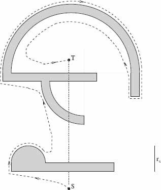
Figure 3.14 Scene 1: Path generated by algorithms VisBug-21 or VisBug-22. The radius of vision is rυ.
Analysis of VisBug-21. Examples shown in Figures 3.14 and 3.15 demonstrate the effect of radius of vision rυ on performance of algorithm VisBug-21. (Compare this with the Bug2 performance in the same environment, Figure 3.13). In the analysis that follows, we first look at the algorithm performance and then address the issue of convergence. Since the path generated by VisBug-21 can diverge significantly from the path that would be produced under the same conditions by algorithm Bug2, it is to be shown that the path-length performance of VisBug-21 is never worse than that of Bug2. One would expect this to be true, and it is ensured by the following lemma.
Lemma 3.6.1. For a given scene and a given set of Start and Target points, the path produced by algorithm VisBug-21 is never longer than that produced by algorithm Bug2.
Proof: Assume the scene and start S and target T points are fixed. Consider the robot's position, Ci, and its corresponding intermediate target, Ti, at step i of the path, i = 0, 1,…. We wish to show that the lemma holds not only for the whole path from S to T, but also for an arbitrary step i of the path. This amounts to showing that the inequality
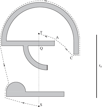
Figure 3.15 Scene 1: Path generated by VisBug-21. The radius of vision rυ is larger than that in Figure 3.14.
holds for any i. The proof is by induction. Consider the initial stage, i = 0; it corresponds to C0 = S. Clearly, |ST0| ≤ [ST0]. This can be written as {SC0} + |C0T0| ≤ [ST0], which corresponds to the inequality (3.15) when i = 0. To proceed by induction, assume that inequality (3.15) holds for step (i − 1) of the path, i > 1:
Each step of the robot's path takes place in one of two ways: either Ci−1 ≠ Ti−1 or Ci−1 = Ti−1. The latter case takes place when the robot moves along the locally convex part of an obstacle boundary; the former case comprises all the remaining situations. Consider the first case, Ci−1 ≠ Ti−1. Here the robot will take a step of length |Ci−1Ci| along a straight line toward Ti−1; Eq. (3.16) can thus be rewritten as
In (3.17), the first two terms form {SCi}, and so
At point Ci the robot will define the next intermediate target, Ti. Now add to (3.18) the obvious inequality |Ti−1Ti| ≤ [Ti−1Ti]:
By the Triangle Inequality, we have
Therefore, it follows from (3.19) and (3.20) that
which proves (3.15).
Consider now the second case, Ci−1 = Ti−1. Here the robot takes a step of length (Ci−1Ci) along the obstacle boundary (the Bug2 path, [Ci−1Ci]). Equation (3.16) becomes
where the left-hand side amounts to {SCi} and the right-hand side to [SCi]. At point Ci, the robot will define the next intermediate target, Ti. Since |CiTi| ≤ [CiTi], inequality (3.22) can be written as
which, again, produces (3.15). Since, by the algorithm's design, at some finite i, Ci = T, then
which completes the proof. Q.E.D.
One can also see from Figure 3.15 that when rυ goes to infinity, algorithm VisBug-21 will generate locally optimal paths, in the following sense. Take two obstacles or two parts of the same obstacle, k and k + 1, that are visited by the robot, in this order. During the robot's passing around obstacle k, once a point on obstacle k + 1 is identified as the next intermediate target, the gap between k and k + 1 will be traversed along the straight line, which presents the locally shortest path.
When defining its intermediate targets, algorithm VisBug-21 could sometimes use points on the M-line that are not necessarily contiguous to the prior intermediate targets. This would result in a more efficient use of robot's vision: By “cutting corners,” the robot would be able to skip some obstacles that intersect the M-line and that it would otherwise have to traverse. However, from the standpoint of algorithm convergence, this is not an innocent operation: It is important to make sure that in such cases the candidate points on the M-line that are “approved” by the algorithm do indeed lie on the Bug2 path.
This is assured by Step 4 of the procedure Compute Ti-21, where a noncontiguous point Q on the M-line is considered a possible candidate for an intermediate target only if the robot's current location C is in the main semiplane. The purpose of this condition is to preserve convergence. We will now show that this arrangement always produces intermediate targets that lie on the Bug2 path.
Consider a current location C of the robot along the VisBug-21 path, a current intermediate target Ti, and some visible point Q on the M-line that is being considered as a candidate for the next intermediate target, Ti+1. Apparently, Q can be accepted as the intermediate target Ti+1 only if it lies further along the Bug2 path than Ti.
Recall that in order to ensure convergence, algorithm Bug2 organizes the set of hit and leave points, Hj and Lj, along the M-line so as to form a sequence of segments
that shrinks to T. This inequality dictates two conditions that candidate points for Q must satisfy in order for VisBug-21 to converge: (i) When the current intermediate target Ti lies on the M-line, then only those points Q should be considered for which |QT| < |TiT|. (ii) When Ti is not on the M-line, it lies on the obstacle boundary, in which case there must be the latest crossing point X between M-line and the obstacle boundary, such that the boundary segment (XTi) is a part of the Bug2 path. In this case, only those points Q should be considered for which |QT| < |XT|. Since points Q, Ti, and X are already known, both of these conditions can be easily checked. Let us assume that these conditions are satisfied. Note that the crossing point X does not necessarily correspond to a hit point for either Bug2 or VisBug-21 algorithms. The following statement holds.
Lemma 3.6.2. For point Q to be further along the Bug2 path than the intermediate target Ti, it is sufficient that the current robot position C lies in the main semiplane.
Proof: Assume that C lies in the main semiplane; this includes a special case when C lies on the M-line. Then, all possible situations can be classified into three cases:
(1) Both Ti and C lie on the M-line.
(2) Ti lies on the M-line, whereas C does not.
(3) Ti does not lie on the M-line. Let us consider each of these cases.
1. Here the robot is moving along the M-line toward T; thus, Ti is between C and T (Figure 3.16a). Since Ti is by definition on the Bug2 path, and both Ti and Q are visible from point C, then point Q must be on the Bug2 path. And, because of condition (i) above, Q must be further along the Bug2 path than Ti.
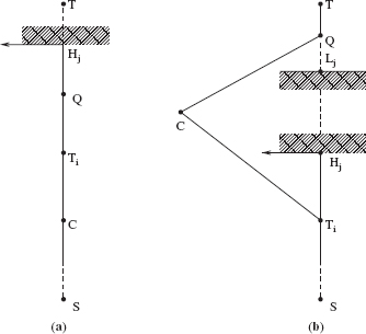
Figure 3.16 Illustration for Lemma 3.6.2: (a) Case 1. (b) Case 2.
2. This case is shown in Figure 3.16b. If no obstacles are crossing the M-line between points Ti and Q, then the lemma obviously holds. If, however, there is at least one such obstacle, then a hit point, Hj, would be defined. By design of the Bug2 algorithm, the line segment TiHj lies on the Bug2 path. At Hj the Bug2 path would turn left and proceed along the obstacle boundary as shown. For each hit point, there must be a matching leave point. Where does the corresponding leave point, Lj, lie?
Consider the triangle TiCQ. Because of the visibility condition, the obstacle cannot cross line segments CTi or CQ. Also, the obstacle cannot cross the line segment TiHj, because otherwise some other hit point would have been defined between Ti and Hj. Therefore, the obstacle boundary and the corresponding segment of the Bug2 path must cross the M-line somewhere between Hj and Q. This produces the leave point Lj. Thereafter, because of condition (i) above, the Bug2 path either goes directly to Q, or meets another obstacle, in which case the same argument applies. Therefore, Q is on the Bug2 path and it is further along this path than Ti.
3. Before considering this case in detail, we make two observations.
Observation 1. Within the assumptions of the lemma, if Ti is not on the M-line, then the current position C of the robot is not on the M-line either. Indeed, if Ti is not on the M-line, then there must exist an obstacle that is responsible for the latest hit point, Hj, and thereafter the intermediate target Ti. This obstacle prevents the robot from seeing any point Q on the M-line that would satisfy the requirement (ii) above.
Observation 2. If point C is not on the M-line, then the line segment |CTi| will never cross the open line segment |HjT| (“open” here means that the segment's endpoints are not included). Here Hj is the lastly defined hit point. Indeed, for such a crossing to take place, Ti must lie in the secondary semiplane (Figure 3.17). For this to happen, the Bug2 path would have to proceed from Hj first into the main semiplane and then enter the secondary semiplane somewhere outside of the line segment |HjT|; otherwise, the leave point, Lj, would be established and the Bug2 path would stay in the main semiplane at least until the next hit point, Hj+1, is defined. Note, however, that any such way of entering the secondary semiplane would produce segments of the Bug2 path that are not contiguous (because of the visibility condition) to the rest of the Bug2 path. By the algorithm, no points on such segments can be chosen as intermediate targets Ti —which means that if the point C is in the main semiplane, then the line segments |CTi| and |HjT| never intersect.

Figure 3.17 Illustration for Lemma 3.6.2: Observation 2.
Situations that fall into the case in question can in turn be divided into three groups:
3a. Point C is located on the obstacle boundary, and C = Ti. This happens when the robot walks along a locally convex obstacle boundary (point C′, Figure 3.18). Consider the curvilinear triangle XjC′Q. Continuing the boundary segment (XjC′) after the point C′, the obstacle (and the corresponding segment of the Bug2 path) will either curve inside the triangle, with |QT| lying outside the triangle (Figure 3.18a), or curve outside the triangle, leaving |QT| inside (Figure 3.18b). Since the obstacle can cross neither the line |CQ| nor the boundary segment (XjC′), it (and the corresponding segment of the Bug2 path) must eventually intersect the M-line somewhere between Xj and Q before intersecting |QT|. The rest of the argument is identical to case 2 above.
3b. Point C is on the obstacle boundary, and C ≠ Ti (Figure 3.18). Consider the curvilinear triangle XjCQ. Again, the obstacle can cross neither the line of visibility |CQ| nor the boundary segment (XjC), and so the obstacle (and the corresponding segment of the Bug2 path) will either curve inside the triangle, with |QT| left outside of it, or curve outside the triangle, with |QT| lying inside. The rest is identical to case 2.
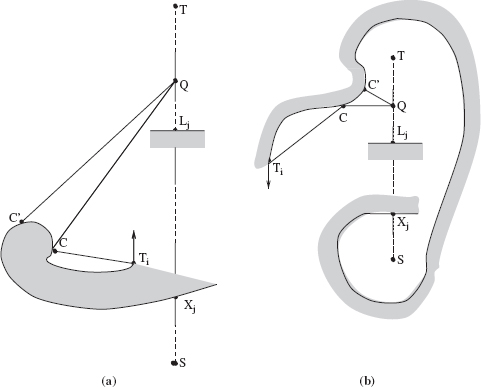
Figure 3.18 Illustration for Lemma 3.6.2: Cases 3a and 3b.
3c. Point C is not on the obstacle boundary. Then, a curvilinear quadrangle is formed, XjTiCQ (Figure 3.19). Again, the obstacle will either curve inside the quadrangle, with |QT| outside of it, or curve outside the quadrangle, with |QT| lying inside. Since neither the lines of visibility |CTi| and |CQ| nor the boundary segment (XjTi) can be crossed, the obstacle (and the corresponding segment of the Bug2 path) will eventually cross |XjQ| before intersecting |QT| and form the leave point Lj. The rest of the argument is identical to case 2. Q.E.D.
If the robot is currently located in the secondary semiplane, then it is indeed possible that a point that lies on the M-line and seems otherwise a good candidate for the next intermediate target T does not lie on the Bug2 path. This means that point should not even be considered as a candidate for T. Such an example is shown in Figure 3.15: While at location C, the robot will reject the seemingly attractive point Q (Step 2 of the algorithm) because it does not lie on the Bug2 path. We are now ready to establish convergence of algorithm VisBug-21.

Figure 3.19 Illustration for Lemma 3.6.2: Case 3c.
Theorem 3.6.1. Algorithm VisBug-21 is convergent.
Proof: By the definition of intermediate target point Ti, for any Ti that corresponds to the robot's location C, Ti is reachable from C. According to the algorithm, the robot's next step is always in the direction of Ti. This means that if the locus of points Ti is converging to T, so will the locus of points C. In turn, we know that if the locus of points Ti lies on the Bug2 path, then it indeed converges to T. The question now is whether all the points Ti generated by VisBug-21 lie on the Bug2 path.
All steps of the procedure Compute Ti-21, except Step 4, explicitly test each candidate for the next Ti for being contiguous to the previous Ti and belonging to the Bug2 path. The only questionable points are points Ti on the M-line that are produced in Step 4 of the procedure: They are not required to be contiguous to the previous Ti. In such cases, points in question are chosen as Ti points only if the robot's location C lies in the main semiplane, in which case the conditions of Lemma 3.6.2 apply. This means that all the intermediate targets Ti generated by algorithm VisBug-21 path lie on the Bug2 path, and therefore converge to T. Q.E.D.
Compared to a tactile sensing-based algorithm, the advantage of using vision is of course in the extra information due to the scene visibility. If the robot is thrown in a crowded scene where at any given moment it can see only a small part of the scene, the efficacy of vision will be obviously limited. Nevertheless, unless the scene is artificially made impossible for vision, one can expect gains from it. This can be seen in performance of VisBug-21 algorithm in the maze borrowed from Section 3.3.2 (see Figure 3.20). For simplicity, assume that the robot's radius of vision goes to infinity. While this ability would be mostly defeated here, the path still looks significantly better than it does under the “tactile” algorithm Bug2 (compare with Figure 3.11).

Figure 3.20 Example of a walk (dashed line) in a maze under Algorithm VisBug-21 (compare with Figure 3.11). S, Start; T, Target.
3.6.3 Algorithm VisBug-22
The structure of this algorithm is somewhat similar to VisBug-21. The difference is that here the robot makes no attempt to ensure that intermediate targets Ti lie on the Bug2 path. Instead, it tries “to shoot as far as possible”; that is, it chooses as intermediate targets those points that lie on the M-line and are as close to the target T as possible. The resulting behavior is different from the algorithm VisBug-21, and so is the mechanism of convergence.
Consider a scene with given Start S and Target T points, and consider a third point, S′, that lies on the M-line somewhere between S and T. Following the term Bug2 path that we used before, we define a quasi-Bug2 path segment as a contiguous segment that starts at S′ and produces a part of the path that algorithm Bug2 would have generated if points S′ and T were its starting and target points, respectively. Because point S′ does not need to be on the Bug2 path, a quasi-Bug2 path segment may or may not be a part of the Bug2 path.
The algorithm VisBug-22 will check points along the Bug2 path or a quasi-Bug2 path segment until the best point on the M-line—that is, one that is the closest to T—is identified. This point S′ then becomes the starting point of another quasi-Bug2 path segment. Then the process repeats. As a result, unlike algorithms Bug2 and VisBug-21, where each hit point has its matching leave point, in VisBug-22 no such matching needs to occur. To be chosen as the starting point S′ of the next quasi-Bug2 path segment, a point must satisfy certain requirements that ensure convergence. These will be considered later, after we describe the whole procedure.
The algorithm includes the Main body, which is identical to that of algorithm VisBug-21 (refer to Section 3.6.2), and the procedure Compute Ti-22. The purpose of the latter is to produce the next intermediate target Ti for a given current position C; it is also responsible for the test for target reachability. Initially, C = S = Ti.
Procedure Compute Ti-22:
- Step 1: If Target T is visible, define Ti = T; procedure stops.
Else if Ti is on an obstacle boundary, go to Step 3.
Else go to Step 2. - Step 2: Define point Q as the endpoint of the maximum-length contiguous segment of the M-line, |Ti Q|, extending from Ti in the direction of T.
If an obstacle has been identified crossing the M-line at point Q, then define a hit point, H = Q; define Ti = Q; go to Step 3.
Else define Ti = Q; go to Step 4. - Step 3: Define point Q as the endpoint of the maximum length contiguous segment of the obstacle boundary, (TiQ), extending from Ti in the local direction.
If an obstacle has been identified crossing the M-line at a point P ∈ (TiQ), |P, T| < |HT|, and line |PT| does not cross the obstacle at P, then define a leave point, L = P, define Ti = P, and go to Step 2.
If the lastly defined hit point H is identified again and H ∈ (TiQ), then the target is not reachable; procedure stops.
Else define Ti = Q; go to Step 4. - Step 4: If Ti is on the M-line, define Q = Ti; otherwise define Q = H.
If points {P} on the M-line are identified such that |S′T| < |QT|, S' ∈ {P}, then find the point S' ∈ {P} that produces the shortest distance |S′T|; define Ti = S′; go to Step 2.
Else the procedure stops.
Performance and Convergence of VisBug-22. The algorithm's performance is demonstrated in Figures 3.14 and 3.21; the values of radius of vision rυ used are the same as in examples for VisBug-21 (Figures 3.14 and 3.15). Compare these with the performance of algorithm Bug2 in the same scene (Figure 3.13). As one can see from Figure 3.14, algorithms VisBug-21 and VisBug-22 can sometimes generate identical paths. This is not so in general. Also, neither algorithm can be said to be superior to the other in all scenes. For example, in one scene algorithm VisBug-21 performs better (Figure 3.15) than algorithm VisBug-22 (Figure 3.21), but luck switches to VisBug-22 in another scene shown in Figure 3.23.
Convergence of algorithm VisBug-22 follows simply from the fact that all the starting points, S′, of the successive quasi-Bug2 path segments lie on the M-line, and they are organized in such a way as to produce a finite sequence of distances shrinking to T :
where points S′ are numbered in the order of their appearance.

Figure 3.21 Scene 1. The path generated by algorithm VisBug-22. The radius of vision rυ here is larger than that in Figure 3.14, and is equal to that in Figure 3.15.
3.7 FROM A POINT ROBOT TO A PHYSICAL ROBOT
So far our mobile robot has been a point. What changes if we try to extend the motion planning algorithms considered in this chapter to real mobile robots with flesh and finite dimensions?5 A theoretically correct way to address this question is to replace the original problem of guiding the robot in the two-dimensional workspace (W-space) with its reflection in the corresponding configuration space (C-space). (This will be done systematically in Chapter 5 when considering the motion planning problem for robot arm manipulators.) C-space is the space of the robot's control variables, its degrees of freedom. In C-space the robot becomes a point. Since our robot has two degrees of freedom, which correspond to its coordinates X and Y in the planar W-space, its C-space is also a plane.6 Obstacles will change accordingly.
If the robot is of a simple convex shape—for example, circular or rectangular, as most mobile robots are, or can be satisfactorily approximated by such shapes—the corresponding C-space can be obtained simply by “growing” the obstacles to compensate for the robot's “shrinking” to a point. This well-known approach has been used already in the earlier works on motion planning (see Section 2.7). For simple robot shapes the C-space is “almost the same” as the W-space, and motion planning can be done in W-space, keeping in mind this transformation. One can see, for example, that asking whether the circular robot R of diameter D shown in Figure 3.22 can pass between two obstacles, O1 and O2, is equivalent to asking if the minimum distance between the grown obstacles, each grown by D/2, is more than zero.
Recall that explicitly building the C-space is possible only in the paradigm of motion planning with complete information (the Piano Mover's model). Since in the SIM paradigm input information is never complete and appears as the robot moves, there is no information to calculate the C-space. One can, however, design algorithms based on C-space properties, and this is what will happen in the following chapters.
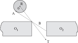
Figure 3.22 Effect of robot shape and geometry on motion planning.
For the practical side of our question, What changes for the algorithms considered in this chapter when applying them to real mobile robots with finite dimensions? the answer is, nothing changes. Recall that the algorithms VisBug make decisions “on the fly,” in real time. They make the robot either (a) move in free space by following the M-line or (b) follow obstacle boundaries. For example, when following an obstacle boundary, if the robot arrives at a gap between two obstacles, it may or may not be able to pass it. If the gap is too narrow for the robot to pass through, it will perceive both obstacles as one. When following the obstacle boundaries, the robot will switch from one obstacle to the other without even noticing this fact.
Additional heuristics can be added to improve the algorithm efficiency, as long as care is taken not to imperil the algorithm convergence. For example, if the robot sees its target T through a gap between two obstacles, it may attempt to measure the width of the gap to make sure that it will be able to pass it, before it actually moves to the gap. Or, if the robot's shape is more complex than a circle, it may try to move through the gap by varying its orientation.
An interesting question appears when studying the effect of location of sensor(s) on the robot body on motion planning. Assume the robot R shown in Figure 3.22 has a range sensor. If the sensor is located at the robot's center then, as the dotted line of vision OT shows, the robot will see the gap between two obstacles and will act accordingly. But, if the sensor happened to be attached to the point A on the robot periphery, then the dotted line AB shows that the robot will not be able to see if the gap is real. The situation can be even more complex: For example, it is not uncommon for real-world mobile robots to have a battery of sonar sensors attached along the circumference of the robot body. Then different sensors may see different objects, the robot's intelligence needs to reconcile those different readings, and a more careful scheme is needed to model the C-space sensing. Little work has been done in this area; some such schemes have been explored by Skewis [64].
3.8 OTHER APPROACHES
Recall the division of all sensor-based motion planning algorithms into two classes (Section 3.5). Class 1 combines algorithms in which the robot never leaves an obstacle unless and until it explores it completely. Class 2 combines algorithms that are complementary to those in Class 1: In them the robot can leave an obstacle and walk further, and even return to this obstacle again at some future time, without exploring it in full.
As mentioned above, today Class 1 includes only one algorithm, Bug1. The reason for this paucity likely lies in the inherent conservatism of algorithms in this Class. Their dogmatically reaching the upper performance bound in the most simple scenes, where a more agile strategy would likely do much better, does not leave much room for creativity. Besides, Bug1 does already reach the universal lower bound (3.13) of the sensor-based motion planning problem, so there is not much one can expect in advancing theory.
Performance aside, one may wonder how much variety there is in Class 1. Most likely not much, but we do not know for sure.
This makes Bug1 an unrivaled champion among “tactile” algorithms—a somewhat ironic title, given that Bug1 is not a likely candidate for real-world robots, except perhaps in special applications. One such application is generation of the outline of a scene in question, which is producing contours of obstacles present in the scene. You supply the robot with a few pairs of S and T points to ensure that it will visit all obstacles of interest, make sure that it stores the files of coordinates while walking around obstacles, and let it go. As a side product of those trips, the robot will bring back a map of the scene. The technique is especially good for obtaining such outlines and contours in a database, with an imaginary point robot. This method of obtaining the map, while not theoretically sound, is quite competitive compared to other techniques.7 With this technique the robot cannot, of course, uncover pieces of free space trapped inside obstacles, unless the robot explicitly starts there.
The situation is more interesting with Class 2 algorithms, including extensions to vision and range sensing. If the Bug family (as some researchers started calling these procedures) is to grow, this will likely be happening in Class 2. Between 1984 and now (1984 being the year of first publications on sensor-based motion planning), over a dozen provable algorithms from this class have been reported in the literature. Besides, many heuristic procedures relying on the “engineering approach” have been described; their convergence and performance properties in arbitrary scenes is anybody's guess.
The following brief review of significant work on provable Class 2 sensor-based algorithms is admittedly incomplete. Ideas similar to those explored in this book—that is, with a focus on topological rather than geometrical properties of space—has been considered by a number of researchers. Algorithms Alg1 and Alg2 by Sankaranarayanan and Vidyasagar [65] successfully fight the unpleasant tendency of the Bug2 algorithm to produce multiple local cycles in some special scenes (see Section 3.5). Whereas local cycles can be stopped via a straightforward combination of Bug1 and Bug2 procedures (see the BugM1 algorithm, Section 3.5), Alg1 and Alg2 do it better and they do it more economically. Importantly, they reach the path length lower bound (3.14) for the Class 2 algorithms, and by doing so they “close” the Class 2 of sensor-based planning algorithms, similar to how Bug1 closes Class 1.
Also in this group are elegant provable algorithms TangentBug [66] by Kamon, Rivlin, and Rimon, and DistBug [67, 68] by Kamon and Rivlin. Algorithm TangentBug, in turn, has inspired procedures WedgeBug and RoverBug [69, 70] by Laubach, Burdick, and Matthies, which try to take into account issues specific for NASA planet rover exploration. A number of schemes with and without proven convergence have been reported by Noborio [71].
Given the practical needs, it is not surprising that many attempts in sensor-based planning strategies focus on distance sensing—stereo vision, laser range sensing, and the like. Some earlier attempts in this area tend to stick to more familiar graph-theoretical approaches of computer science, and consequently treat space in a discrete rather than continuous manner. A good example of this approach is the visibility-graph based approach by Rao et al. [72].
Standing apart is the approach described by Choset et al. [73, 74], which can be seen as an attempt to fill the gap between the two paradigms, motion planning with complete information (Piano Mover's model) and motion planning with incomplete information [other names are sensor-based planning, or Sensing–Intelligence–Motion (SIM)]. The idea is to use sensor-based planning to first build the map and then the Voronoi diagram of the scene, so that the future robot trips in this same area could be along shorter paths—for example, along links of the acquired Voronoi diagram. These ideas, and applications that inspire them, are different from the go-from-A-to-B problem considered in this book and thus beyond our scope. They are closer to the systematic space exploration and map-making. The latter, called in the literature terrain acquisition or terrain coverage, might be of use in tasks like robot-assisted map-making, floor vacuuming, lawn mowing, and so on (see, e.g., Refs. 1 and 75).
While most of the above works provide careful analysis of performance and convergence, the “engineering approach” heuristics to sensor-based motion planning procedures usually discuss their performance in terms of “consistently better than” or “better in our experiments,” and so on. Since idiosyncracies of these algorithms are rarely analyzed, their utility is hard to assess. There have been examples when an algorithm published as provable turned out to be ruefully divergent even in simple scenes.8
Related to the area of two-dimensional motion planning are also works directed toward motion planning for a “point robot” moving in three-dimensional space. Note that the increase in dimensionality changes rather dramatically the formal foundation of the sensor-based paradigm. When moving in the (two-dimensional) plane, if the point robot encounters an obstacle, it has a choice of only two ways to pass around it: from the left or from the right, clockwise or counterclockwise. When a point robot encounters an object in the three-dimensional space, it is faced with an infinite number of directions for passing around the object. This means that unlike in the two-dimensional case, the topological properties of three-dimensional space cannot be used directly anymore when seeking guarantees of algorithm completeness.
Accordingly, objectives of works in this area are usually toward complete exploration of objects. One such application is visual exploration of objects (see, e.g., Refs. 63 and 76): One attempts, for example, to come up with an economical way of automatically manipulating an object on the supermarket counter in order to locate on it the bar code.
Extending our go-from-A-to-B problem to the mobile robot navigation in three-dimensional space will likely necessitate “artificial” constraints on the robot environment (which we were lucky not to need in the two-dimensional case), such as constraints on the shapes of objects, the robot's shape, some recognizable properties of objects' surfaces, and so on. One area where constraints appear naturally, as part of the system kinematic design, is motion planning for three-dimensional arm manipulators. The very fact that the arm links are tied into some kinematic structure and that the arm's base is bolted to its base provide additional constraints that can be exploited in three-dimensional sensor-based motion planning algorithms. This is an exciting area, with much theoretical insight and much importance to practice. We will consider such schemes in Chapter 6.
3.9 WHICH ALGORITHM TO CHOOSE?
With the variety of existing sensor-based approaches and algorithms, one is entitled to ask a question: How do I choose the right sensor-based planning algorithm for my job? When addressing this question, we can safely exclude the Class 1 algorithms: For the reasons mentioned above, except in very special cases, they are of little use in practice.
As to Class 2, while usually different algorithms from this group produce different paths, one would be hard-pressed to recommend one of them over the others. As we have seen above, if in a given scene algorithm A performs better than algorithm B, their luck may reverse in the next scene. For example, in the scene shown in Figures 3.15 and 3.21, algorithm VisBug-21 outperforms algorithm VisBug-22, and then the opposite happens in the scene shown in Figure 3.23. One is left with an impression that when used with more advanced sensing, like vision and range finders, in terms of their motion planning skills just about any algorithm will do, as long as it guarantees convergence.
Some people like the concept of a benchmark example for comparing different algorithms. In our case this would be, say, a fixed benchmark scene with a fixed pair of start and target points. Today there is no such benchmark scene, and it is doubtful that a meaningful benchmark could be established. For example, the elaborate labyrinth in Figure 3.11 turns out to be very easy for the Bug2 algorithm, whereas the seemingly simpler scene in Figure 3.6 makes the same algorithm produce a torturous path. It is conceivable that some other algorithm would have demonstrated an exemplary performance in the scene of Figure 3.6, only to look less brave in another scene. Adding vision tends to smooth algorithms' idiosyncracies and to make different algorithms behave more similarly, especially in real-life scenes with relatively simple obstacles, but the said relationship stays.
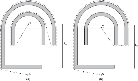
Figure 3.23 Scene 2. Paths generated (a) by algorithm VisBug-21 and (b) by algorithm VisBug-22.
Furthermore, even seemingly simple questions—(1) Does using vision sensing guarantee a shorter path compared to using tactile sensing? or (2) Does a better (that is, farther) vision buy us better performance compared to an inferior (that is, more myopic) vision?—have no simple answers. Let us consider these questions in more detail.
1. Does using vision sensing guarantee a shorter path compared to using tactile sensing? The answer is no. Consider the simple example in Figure 3.24. The robot's start S and target T points are very close to and on the opposite sides of the convex obstacle that lies between them. By far the main part of the robot path will involve walking around the obstacle. During this time the robot will have little opportunity to use its vision because at every step it will see only a tiny piece of the obstacle boundary; the rest of it will be curving “around the corner.”
So, in this example, robot vision will behave much like tactile sensing. As a result, the path generated by algorithm VisBug-21 or VisBug-22 or by some other “seeing” algorithm will be roughly no shorter than a path generated by a “tactile” algorithm, no matter what the robot's radius of vision rυ is. If points S and T are further away from the obstacle, the value of rυ will matter more in the initial and final phases of the path but still not when walking along the obstacle boundary.
When comparing “tactile” and “seeing” algorithms, the comparative performance is easier to analyze for less opportunistic algorithms, such as VisBug-21: Since the latter emulates a specific “tactile” algorithm by continuously short-cutting toward the furthest visible point on that algorithm's path, the resulting path will usually be shorter, and never longer, than that of the emulated “tactile” algorithm (see, e.g., Figure 3.14).

Figure 3.24 In this scene, the path generated by an algorithm with vision would be almost identical to the path generated by a “tactile” planning algorithm.
With more opportunistic algorithms, like VisBig-22, even this property breaks down: While paths that algorithm VisBig-22 generates are often significantly shorter than paths produced by algorithm Bug2, this cannot be guaranteed (compare Figures 3.13 and 3.21).
2. Does better vision (a larger radius of vision, rυ) guarantee better performance compared to an inferior vision (a smaller radius of vision)? We know already that for VisBug-22 this is definitely not so—a larger radius of vision does not guarantee shorter paths (compare Figures 3.21 and 3.14). Interestingly, even for a more stable VisBug-21, it is not so. The example in Figure 3.25 shows that, while VisBug-21 always does better with vision than with tactile sensing, more vision—that is, a larger rυ—does not necessarily buy better performance. In this scene the robot will produce a shorter path when equipped with a smaller radius of vision (Figures 3.25a) than when equipped with a larger radius of vision (Figures 3.25b).
The problem lies, of course, in the fundamental properties of uncertainty. As long as some, even a small piece, of relevant information is missing, anything may happen. A more experienced hiker will often find a shorter path, but once in a while a beginner hiker will outperform an experienced hiker. In the stock market, an experienced stock broker will usually outperform an amateur investor, but once in a while their luck will reverse.9 In situations with uncertainty, more experience certainly helps, but it helps only on the average, not in every single case.

Figure 3.25 Performance of algorithm VisBug-21 in the same scene (a) with a smaller radius of vision and (b) with a larger radius of vision. The smaller (worse) vision results in a shorter path!
These examples demonstrate the variety of types of uncertainty. Notice another interesting fact: While the experienced hiker and experienced stock broker can make use of a probabilistic analysis, it is of no use in the problem of motion planning with incomplete information. A direction to pass around an obstacle that seems to promise a shorter path to the target may offer unpleasant surprises around the corner, compared to a direction that seemed less attractive before but is objectively the winner. It is far from clear how (and whether) one can impose probabilities on this process in any meaningful way. That is one reason why, in spite of high uncertainty, sensor-based motion planning is essentially a deterministic process.
3.10 DISCUSSION
The somewhat surprising examples above (see the last few figures in the previous section) suggest that further theoretical analysis of general properties of Class 2 algorithms may be of more benefit to science and engineering than proliferation of algorithms that make little difference in real-world tasks. One interesting possibility would be to attempt a meaningful classification of scenes, with a predictive power over the performance of various algorithmic schemes. Our conclusions from the worst-case bounds on algorithm performance also beg for a similar analysis in terms of some other, perhaps richer than the worst-case, criteria.
This said, the material in this chapter demonstrates a remarkable success in the last 10–15 years in the state of the art in sensor-based robot motion planning. In spite of the formidable uncertainty and an immense diversity of possible obstacles and scenes, a good number of algorithms discussed above guarantee convergence: That is, a mobile robot equipped with one of these procedures is guaranteed to reach the target position if the target can in principle be reached; if the target is not reachable, the robot will make this conclusion in finite time. The algorithms guarantee that the paths they produce will not circle in one area an indefinite number of times, or even a large number of times (say, no more than two or three).
Twenty years ago, most specialists would doubt that such results were even possible. On the theoretical level, today's results mean, to much surprise from the standpoint of earlier views on the subject, that purely local input information is not an obstacle to obtaining global solutions, even in cases of formidable complexity.
Interesting results raise our appetite for more results. Answers bring more questions, and this is certainly true for the area at hand. Below we discuss a number of issues and questions for which today we do not have answers.
Bounds on Performance of Algorithms with Vision. Unlike with “tactile” algorithms, today there are no upper bounds on performance of motion planning algorithms with vision, such as VisBug-21 or VisBug-22 (Section 3.6). While from the standpoint of theory it would be of interest to obtain bounds similar to the bound (3.13) for “tactile” algorithms, they would likely be of limited generality, for the following reasons.
First, to make such bounds informative, we would likely want to incorporate into them characteristics of the robot's vision—at least the radius of vision rυ, and perhaps the resolution, accuracy, and so on. After all, the reason for developing these bounds would be to know how vision affects robot performance compared to the primitive tactile sensing. One would expect, in particular, that vision improves performance. As explained above, this cannot be expected in general. Vision does improve performance, but only “on the average,” where the meaning of “average” is not clear. Recall some examples in the previous section: In some scenes a robot with a larger radius of vision rυ will perform worse than a robot with a smaller rυ. Making the upper bound reflect such idiosyncrasies would be desirable but also difficult.
Second, how far the robot can see depends not only on its vision but also on the scene it operates in. As the example in Figure 3.24 demonstrates, some scenes can bring the efficiency of vision to almost that of tactile sensing. This suggests that characteristics of the scene, or of classes of scenes, should be part of the upper bounds as well. But, as geometry does not like probabilities, the latter is not a likely tool: It is very hard to generalize on distributions of locations and shapes of obstacles in the scene.
Third, given a scene and a radius of vision rυ, a vastly different path performance will be produced for different pairs of start and target points in that same scene.
Moving Obstacles. The model of motion planning considered in this chapter (Section 3.1) assumes that obstacles in the robot's environment are all static—that is, do not move. But obstacles in the real world may move. Let us call an environment where obstacles may be moving the dynamic (changing, time-sensitive) environment. Can sensor-based planning strategies be developed capable of handling a dynamic environment? Even more specifically, can strategies that we developed in this chapter be used in, or modified to account for, a dynamic environment?
The answer is a qualified yes. Since our model and algorithms do not include any assumptions about specifics of the geometry and dimensions of obstacles (or the robot itself), they are in principle ideally suited for handling a dynamic environment. In fact, one can use the Bug and VisBug family algorithms in a dynamic environment without any changes. Will they always work? The answer is, “it depends,” and the reason for the qualified answer is easy to understand.
Assume that our robot moves with its maximum speed. Imagine that while operating under one of our algorithms—it does not matter which one—the robot starts passing around an obstacle that happens to be of more or less complex shape. Imagine also that the obstacle itself moves. Clearly, if the obstacle's speed is higher than the speed of the robot, the robot's chance to pass around the obstacle and ever reach the target is in doubt. If on top of that the obstacle happens to also be rotating, so that it basically cancels the robot's attempts to pass around it, the answer is not even in doubt: The robot's situation is hopeless.
In other words, the motion parameters of obstacles matter a great deal. We now have two options to choose from. One is to use algorithms as they are, but drop the promise of convergence. If the obstacles' speeds are low enough compared to the robot, or if obstacles move more or less in one place, like a tree in the wind, then the robot will likely get where it intends. Even if obstacles move faster than the robot, but their shapes or directions of motion do not create situations as in the example above, the algorithms will still work well. But, if the situation is like the one above, there will be no convergence.
Or we can choose another option. We can guarantee convergence of an algorithm, but impose some additional constraints on the motion of objects in the robot workspace. If a specific environment satisfies our constraints, convergence is guaranteed. The softer those constraints, the more universal the resulting algorithms. There has been very little research in this area.
For those who need a real-world incentive for such work, here is an example. Today there are hundreds of human-made dead satellites in the space around Earth. One can bet that all of them have been designed, built, and launched at high cost. Some of them are beyond repair and should be hauled to a satellite cemetery. Some others could be revived after a relatively simple repair—for example, by replacing their batteries. For long time, NASA (National Aeronautics and Space Administration) and other agencies have been thinking of designing a robot space vehicle capable of doing such jobs.
Imagine we designed such a system: It is agile and compact; it is capable of docking, repair, and hauling of space objects; and, to allow maneuvering around space objects, it is equipped with a provable sensor-based motion planning algorithm. Our robot—call it R-SAT—arrives to some old satellite “in a coma”—call it X. The satellite X is not only moving along its orbit around the Earth, it is also tumbling in space in some arbitrary ways. Before R-SAT starts on its repair job, it will have to fly around X, to review its condition and its useability. It may need to attach itself to the satellite for a more involved analysis. To do this—fly around or attach to the satellite surface—the robot needs to be capable of speeds that would allow these operations.
If the robot arrives at the site without any prior analysis of the satellite X condition, this amounts to our choosing the first option above: No convergence of R-SAT motion planning around X is guaranteed. On the other hand, a decision to send R-SAT to satellite X might have been made after some serious remote analysis of the X's rate of tumbling. The analysis might have concluded that the rate of tumbling of satellite X was well within the abilities of the R-SAT robot. In our terms, this corresponds to adhering to the second option and to satisfying the right constraints—and then the R-SAT's motion planning will have a guaranteed convergence.
Multirobot Groups. One area where the said constraints on obstacles' motion come naturally is multirobot systems. Imagine a group of mobile robots operating in a planar scene. In line with our usual assumption of a high level of uncertainty, assume that the robots are of different shapes and the system is highly decentralized. That is, each robot makes its own motion planning decisions without informing other robots, and so each robot knows nothing about the motion planning intentions of other robots. When feasible, this type of control is very reliable and well protected against communication and other errors.
A decentralized control in multirobot groups is desirable in many settings. For example, it would be of much value in a “robotic” battlefield, where a continuous centralized control from a single commander would amount to sacrificing the system reliability and fault tolerance. The commander may give general commands from time to time—for instance, on changing goals for the whole group or for specific robots (which is an equivalent of prescribing each robot's next target position)—but most of the time the robots will be making their own motion planning decisions.
Each robot presents a moving obstacle to other robots. (Then there may also be static obstacles in the workspace.) There is, however, an important difference between this situation and the situation above with arbitrary moving obstacles. You cannot have any beforehand agreement with an arbitrary obstacle, but you can have one with other robots. What kind of agreement would be unconstraining enough and would not depend on shapes and dimensions and locations? The system designers may prescribe, for example, that if two robots meet, each robot will attempt to pass around the other only clockwise. This effectively eliminates the above difficulty with the algorithm convergence in the situation with moving obstacles.10 (More details on this model can be found in Ref. 77.)
Needs for More Complex Algorithms. One area where good analysis of algorithms is extremely important for theory and practice is sensor-based motion planning for robot arm manipulators. Robot manipulators operate sometimes in a two-dimensional space, but more often they operate in the three-dimensional space. They have complex kinematics, and they have parts that change their relative positions in complex ways during the motion. Not rarely, their workspace is filled with obstacles and with other machinery (which is also obstacles).
Careful motion planning is essential. Unlike with mobile robots, which usually have simple shapes and can be controlled in an intuitively clear fashion, intuition helps little in designing new algorithms or even predicting the behavior of existing algorithms for robot arm manipulators.
As mentioned above, performance of Bug2 algorithm deteriorates when dealing with situations that we called in-position. In fact, this will be likely so for all Class 2 motion planning algorithms. Paths tend to become longer, and the robot may produce local cycles that keep “circling” in some segments of the path. The chance of in-position situations becomes very persistent, almost guaranteed, with arm manipulators. This puts a premium on good planning algorithms. This area is very interesting and very unintuitive. Recall that today about 1,000,000 industrial arms manipulators are busy fueling the world economy. Two chapters of this book, Chapters 5 and 6, are devoted to the topic of sensor-based motion planning for arm manipulators.
The importance of motion planning algorithms for robot arm manipulators is also reinforced by its connection to teleoperation systems. Space-operator-guided robots (such as arm manipulators on the Space Shuttle and International Space Station), robot systems for cleaning nuclear reactors, robot systems for detonating mines, and robot systems for helping in safety operations are all examples of teleoperation systems. Human operators are known to make mistakes in such tasks. They have difficulty learning necessary skills, and they tend to compensate difficulties by slowing the operation down to crawling. (Some such problems will be discussed in Chapter 7.) This rules out tasks where at least a “normal” human speed is a necessity.
One potential way out of this difficulty is to divide responsibilities between the operator and the robot's own intelligence, whereby the operator is responsible for higher-level tasks—planning the overall task, changing the plan on the fly if needed, or calling the task off if needed—whereas the lower-level tasks like obstacle collision avoidance would be the robot's responsibility. The two types of intelligence, human and robot intelligence, would then be combined in one control system in a synergistic manner. Designing the robot's part of the system would require (a) the type of algorithms that will be considered in Chapters 5 and 6 and (b) sensing hardware of the kind that we will explore in Chapter 8.
Turning back to motion planning algorithms for mobile robots, note that nowhere until now have we talked about the effect of robot dynamics on motion planning. This implicitly assumed, for example, that any sharp turn in the robot's path dictated by the planning algorithm was deemed feasible. For a robot with flesh and reasonable mass and speed, this is of course not so. In the next chapter we will turn to the connection between robot dynamics and motion planning.
3.11 EXERCISES
- Recall that in the so-called out-position situations (Section 3.3.2) the algorithm Bug2 has a very favorable performance: The robot is guaranteed to have no cycles in the path (i.e., to never pass a path segment more than once). On the other hand, the in-position situations can sometimes produce long paths with local cycles. For a given scene, the in-position was defined in Section 3.3.2 as a situation when either Start or Target points, or both, lie inside the convex hull of obstacles that the line (Start, Target) intersects. Note that the in-position situation is only a sufficient condition for trouble: Simple examples can be designed where no cycles are produced in spite of the in-position condition being satisfied.
Try to come up with a necessary and sufficient condition—call it GOODCON—that would guarantee a no-cycle performance by Bug2 algorithm. Your statement would say: “Algorithm Bug2 will produce no cycles in the path if and only if condition GOODCON is satisfied.”
- The following sensor-based motion planning algorithm, called AlgX (see the procedure below), has been suggested for moving a mobile point automaton (MA) in a planar environment with unknown arbitrarily shaped obstacles. MA knows its own position and that of the target location T, and it has tactile sensing; that is, it learns about an obstacle only when it touches it. AlgX makes use of the straight lines that connect MA with point T and are tangential to the obstacle(s) at the MA's current position.
The questions being asked are:
- Does AlgX converge?
- If the answer is “yes,” estimate the performance of AlgX.
- If the answer is “no,” why not? Explain and give a counterexample. Using the same idea of the tangential lines connecting MA and T, try to fix the algorithm. Your procedure must operate with finite memory. Estimate its performance.
- Develop a test for target reachability.
Just like the Bug1 and Bug2 algorithms, the AlgX procedure also uses the notions of (a) hit points, Hj, and leave points, Lj, on the obstacle boundaries and (b) local directions. Given the start S and target T points, here are some necessary details:
- Point P becomes a hit point when MA, while moving along the ST line, encounters an obstacle at P.
- Point P can become a leave point if and only if (1) it is possible for MA to move from P toward T and (2) there is a straight line that is tangential to the obstacle boundary at P and passes through T. When a leave point is encountered for the first time, it is called open; it may be closed by MA later (see the procedure).
- A local direction is the direction of following an obstacle boundary; it can be either left or right. In AlgX the current local direction is inverted whenever MA passes through an open leave point; it does not change when passing through a closed leave point.
- A local cycle is formed when MA visits some points of its path more than once.
The idea behind the algorithm AlgX is as follows. MA starts by moving straight toward point T. Every time it encounters an obstacle, it inverts its local direction, the idea being that this will keep it reasonably close to the straight line (S, T). If a local cycle is formed, MA blames it on the latest turn it made at a hit point. Then MA retraces back to the latest visited leave point, closes it, and whence takes the opposite turn at the next hit point. If that turn leads again to a local cycle, then the turn that led to the current leave point is to be blamed. And so on. The procedure operates as follows:
Initialization. Set the current local direction to “right”; set j = 0, Lj = S.
Step 1. Move along a straight line from the current leave point toward point T until one of the following occurs:
- Target T is reached; the procedure terminates.
- An obstacle is encountered; go to Step 2.
Step 2. Define a hit point Hj. Turn in the current local direction and move along the obstacle boundary until one of the following occurs:
- Target T is reached; the procedure terminates.
- The current velocity vector (line tangential to the obstacle at the current MA position) passes through T, and this point has not been defined previously as a leave point; then, go to Step 3.
- MA comes to a previously defined leave point Li, i ≤ j (i.e., a local cycle has been formed). Go to Step 4.
Step 3. Set j = j + 1; define the current point as a new open leave point; invert the current local direction; go to Step 1.
Step 4. Close the open leave point Lk visited immediately before Li. Invert the local direction. Retrace the path between Li and Lk. (During retracing, invert the local direction when passing through an open leave point, but do not close those points; ignore closed leave points.) Now MA is at the closed leave point Lk. If Li is open, go to Step 1. If Li is closed, execute the second part of Step 2, “…move along…until…,” using the current local direction.
Figure 3.E.2
In Figure 3.E.2, L1 is self-closed because when it is passed for the second time, the latest visited open leave point is L1 itself; L4 is closed when L3 is passed for the second time; no other leave points are closed. When retracing from L3 to L4, the leave point L3 causes inversion of the local direction, but does not close any leave points.
- Design two examples that would result in the best-case and the worst-case performance, respectively, of the Bug2 algorithm. In both examples the same three C-shaped obstacles should be used, and an M-line that connects two distinct points S and T and intersects all three obstacles. An obstacle can be mirror image reversed or rotated if desired. Obstacles can touch each other, in which case they become one obstacle; that is, a point robot will not be able to pass between them at the contact point(s). Evaluate the algorithm's performance in each case.

1In practice, while obtaining the optimal solution is often too computationally expensive, the ever-increasing computer speeds make this feasible for more and more problems.
2In Section 3.5 we will learn of a lower bound that is better and tighter: P ≥ D + 1.5 Σi pi − δ. The proof of that bound is somewhat involved, so in order to demonstrate the underlying ideas we prefer to consider in detail the easier proof of the bound (3.1).
3We will see later that out-position situations are a rarity for arm manipulators.
4To fit the common convention of maze search literature, we present a discrete version of the continuous path planning problem: The maze is a rectangular cell structure, with each cell being a little square; any cell crossed by the M-line (straight line (S, T)) is considered to be lying on the line. This same discussion can be carried out using an arbitrary curvilinear maze.
5A related question is, What kind of sensing does such a robot need in order to protect its whole body from potential collisions? This will be considered in more detail in Chapters 5 and 8.
6Including other control variables—for example, the robot orientation—would make C-space three or even higher-dimensional and will complicate the problem accordingly. In practice, the effect of orientation can be often considered independent from the translation controls in X and Y directions. Then the said complication can be avoided. These more special questions are not pursued in this text. Some of these are discussed in Ref. 64.
7This is not to suggest that Bug1 is an algorithm for map-making. Map-making (terrain acquisition and terrain coverage are other terms one finds in literature) is a different problem. See, for example, Ref. 1.
8As the principles of design of motion planning algorithms have become clearer, in the last 10–15 years the level of sophistication has gone up significantly. Today the homework in a graduate course on motion planning can include an assignment to design a new provable sensor-based algorithm, or to decide if some published algorithm is or is not convergent.
9On a quick glance, the same principle seems to apply to the game of chess, but it does not. Unlike in other examples above, in chess the uncertainty comes not from the lack of information—complete information is right there on the table, available to both players—but from the limited amount of information that one can process in limited time. In a given time an experienced player will check more candidate moves than will a novice.
10Note that this is the spirit of the automobile traffic rules.
Sensing, Intelligence, Motion, by Vladimir J. Lumelsky
Copyright © 2006 John Wiley & Sons, Inc.