Chapter 5: Setting Up an Environment with Geometry Nodes

In the last three chapters, we worked toward making a non-realistic render. We covered some material editing, lighting, camera work, and rendering to get the most out of EEVEE to make a cartoony house-in-a-cloud. Now, we're going to up the ante and make an outdoor environment using some premade grass and rocks, as well as looking at some advanced aspects of Blender, including Geometry Nodes, which will be covered in this chapter.

Blender hasn't always been the computer graphics powerhouse that it is now. Thanks to diligent work from many amazing developers, Blender users get to work with many new and interesting tools, as Blender is constantly updated and changed so that it is the very best software that it can be. One such tool is Geometry Nodes. Added to Blender in 2020, Geometry Nodes is a system of nodes that we can string together to create geometry. The Blender Material Editor that we used in Chapter 2, Creating Materials Fast with EEVEE, operates on the same principle, using nodes that we can string together to create something – in that case, materials. So, you already have some experience in this style of working! I find that many 3D programs are moving toward implementing (or already have implemented!) the same kind of system that Geometry Nodes works on. As a result, learning how to use Geometry Nodes will be very helpful if you ever decide to learn Houdini, Unreal, or any other number of programs that have node systems. Geometry Nodes is flexible, easy to understand, and will be useful in any number of projects you undertake in your career. Let's jump right in and start using it to create a procedural dispersal system for the grass that will be growing on top of our land.

In this chapter, we will cover the following:

• Setting up the scene – adding grass and rocks to the Asset Browser
• Creating a Geometry Nodes system to scatter our objects
• Adding more complexity and applying a modifier to other objects

Technical requirements

Make sure to download the file from GitHub called MiniProject2_Start.blend.

We'll use this as our main .blend file and add more things to it. As you can see, it already has a landscape, water plane, camera, and sun set up inside of it. We covered all these aspects in the last three chapters, so I don't want to repeat the information already presented there. Feel free to poke around the project and see how things work and how I've applied the previously covered principles to this file.

The other files we need to download for this chapter are the grass and rock assets. I find that recreating rocks and grass every time you need them is very tedious and doesn't really teach much. So, we're going to download Nature_Assets.blend, and make sure you have them saved in a place you'll be able to find them. Don't worry about opening them; we can transfer objects between files very easily with the Asset Manager. As with the previous chapter, most of the textures I will be using are downloaded from Ambientcg.com; they have an amazingly vast library of CC0 textures that you can use for free and without attribution. You may consider donating to their cause if you find them as useful as I do.

Grass and Nature Resources

After you've made one rock, you've made them all. I recommend trying to create pieces of nature (trees, rocks, grass, and so on) at least once or twice so that you get the hang of it, but overall, they're very time-consuming and really, really hard to do well. If you have a little bit of money to spend on assets or add-ons, buying grass and trees is a good idea. They are always going to look so much better (3D add-on developers have the time and energy to spend making sure that trees look perfect!) and save you time. To me, and many others, it's way worth the money to skip that part of developing a nature scene. So, don't waste hundreds of hours perfecting your trees when the forest is the more important part.

The supporting files for this chapter can be found here: https://github.com/PacktPublishing/Shading-Lighting-and-Rendering-with-Blenders-EEVEE/tree/main/Chapter05.

Setting up the scene – adding grass and rocks to the Asset Browser

In this section, we'll look at importing the assets that we just downloaded to the main Mini-Project2 scene that we'll be working with in this chapter and setting up the scene so that we can get to the fun stuff – Geometry Nodes! The Asset Browser is a brand-new addition to Blender 3.0, and we're going to use it to add the assets we downloaded to the main scene and also make them available in any other .blend file on our computer.

The first thing we'll do is mark the nature assets as Assets, which then lets us add them to a library that we can reuse at any point:

1. Create a folder in the file explorer you use that you'll easily have access to. I created one in my Documents folder called Blender Assets:

Figure 5.1: An empty folder to use as an asset library

2. Copy the Nature_Assets.blend file to the new folder you just made.
3. Open the Nature_Assets.blend file. You'll see we have two rocks and one grass object:

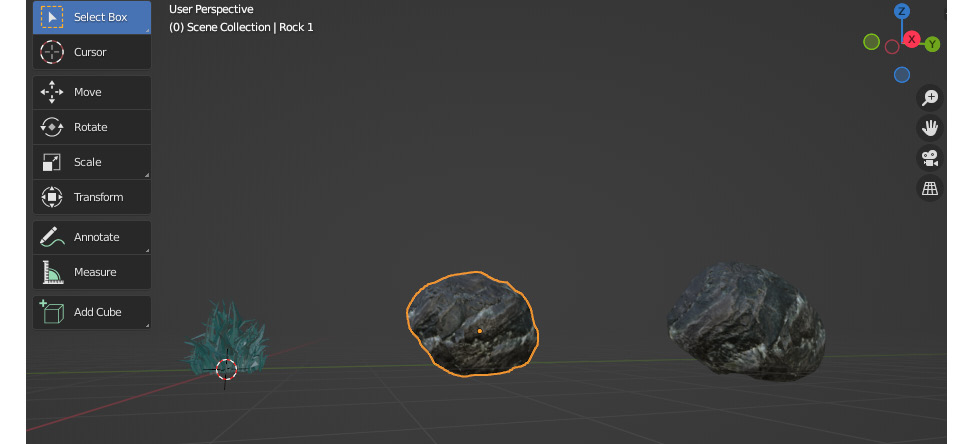
Figure 5.2: Objects in the Nature_Assets.blend file

4. Select an object and then go to the Outliner at the top-right corner; right-click on the object, and then click Mark as Asset. This tells Blender that we want to make the object available for the asset library:

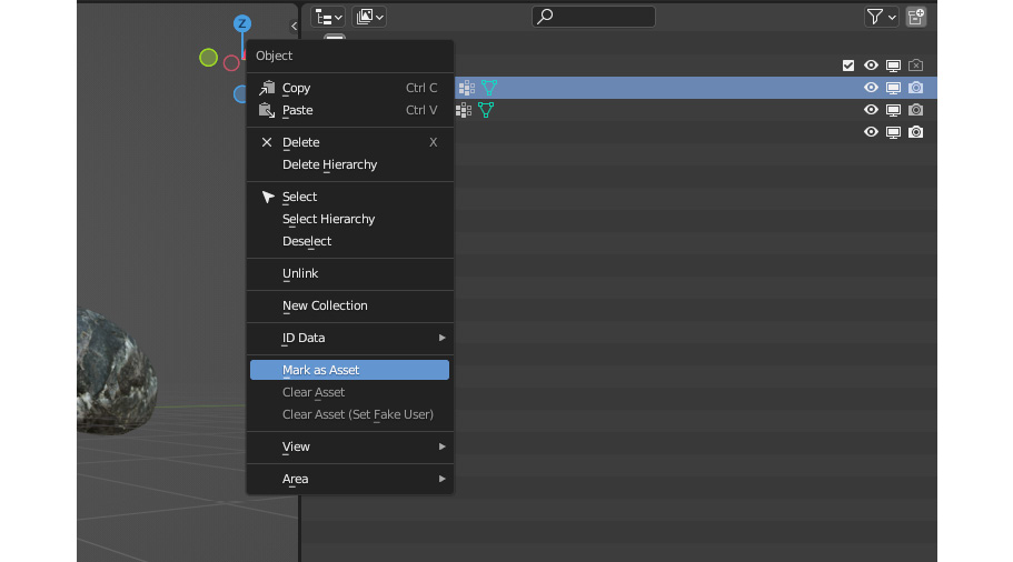
Figure 5.3: The Mark as Asset option

5. Right-click the other two objects in turn and mark each one as an asset. Each object should have a little bookshelf icon next to it now that denotes it has been marked as an asset:

Figure 5.4: The bookshelf icon

Save the Nature_Assets.blend file and close it. We'll now open the Mini-Project 2-Start.blend file.

To import the marked assets into the Mini-Project 2-Start.blend file, we need to tell Blender where to look for our assets:

1. In the toolbar, select the Edit menu and then select Preferences...:

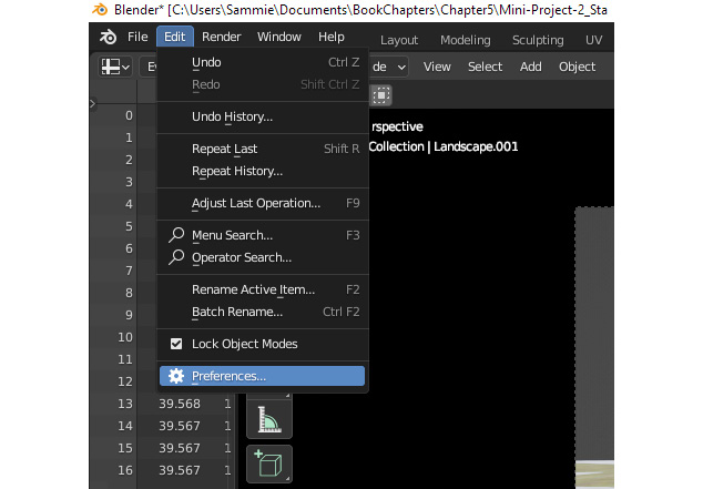
Figure 5.5: Opening the Blender Preferences menu

2. Navigate to the File Paths section in the Blender Preferences menu. At the bottom of the options in the File Path section, there is an option to add a path to Asset Libraries. Either copy and paste the path into the box or use the folder button on the side of the box to navigate to the right folder:
   

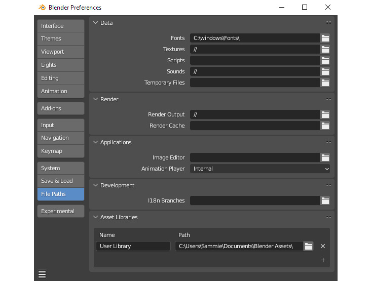
Figure 5.6: The File Paths options

3. In the left window, use the window editor type button to change the window type to Asset Browser:

Figure 5.7: Changing the window to the Asset Browser

The window you just opened will be blank; we just need to change the asset library source from Current File to the asset library we just designated:

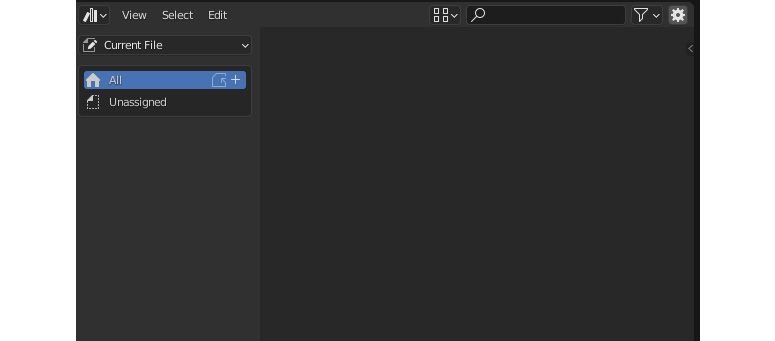
Figure 5.8: The asset library upon first opening

4. Click on the Current File dropdown and change it to User Library:

Figure 5.9: Changing to a user library

You should now see the three files that we marked as assets:

Figure 5.10: The marked assets in our library

5. To import the assets into the scene, all you have to do is drag and drop the assets into the open 3D window:

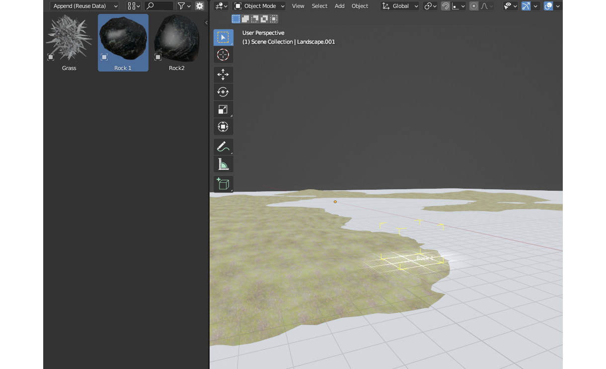
Figure 5.11: Adding the rock asset to the scene

Drag and drop all three objects into the scene:

Figure 5.12: The assets in the scene

This method of adding objects into a scene may seem like more work now, but the effort pays dividends. You can add as many .blend files as you like into the Blender Assets folder that we just created, mark any type of data as an asset, and then reuse it on any file you want! This means that if you spend the time creating a robust library, you can have access to any object you've ever made with ease. This asset library addition to Blender 3.0 is a game-changer, but another game-changer in Blender 3.0 is Geometry Nodes. We'll scatter these three objects with the Geometry Nodes modifier in the next chapter. Don't worry if you've never used Geometry Nodes before; we'll be starting from a beginner level, since Geometry Nodes is new for everyone who uses Blender.

In the upcoming section, we'll go over the Geometry Nodes workspace, the workflow, and how to create flexible node trees to scatter objects on top of a landscape.

Setting up the scene – adding grass and rocks

The first step in using Geometry Nodes is getting access to the Geometry Nodes workspace. Luckily, Blender has a handy workspace tab already set up for us. It's at the top of the screen, in the same row as the Shading workspace tab that we already accessed:

Figure 5.13: Geometry Nodes workspace

After clicking on it, you should have a workspace similar to the following visible, with a Spreadsheet window at the top left, the 3D viewport at the top right, and the Geometry Node editor at the bottom of the screen:

Figure 5.14 : The Geometry Nodes workspace layout

Let's start by adding a new Geometry Nodes network. This works similarly to the material network that we covered in Chapter 2, Creating Materials Fast with EEVEE:

1. The first thing to do is select the object we want to apply the Geometry Nodes modifier to. Since we want to distribute the objects around the landscape, we'll select the Landscape object in our Outliner.
2. Click the New button on the Geometry Nodes menu:

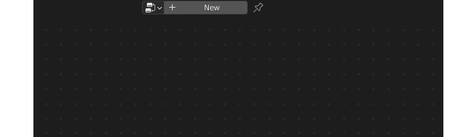
Figure 5.15: The New button on the Geometry Nodes work area

3. We should now have a Geometry Nodes modifier added to the object and be able to see Group Input and Group Output generated as default for Geometry Nodes:

Figure 5.16: Input and output defaults for the new Geometry Nodes system

4. The next thing we want to do is add scattered points to the Geometry Nodes network so that we can then tell Blender that we want to add a Grass object to every scattered point on the landscape. Let's add a node, using Shift + A. Instead of looking through the different node categories to find that node, we can just type the title of the node into the search bar at the top of the Add menu. Let's add a Distribute Points on Faces node. By dropping the node on the line connecting Group Input to Group Output, we can effectively scatter points on top of the surface of our object:

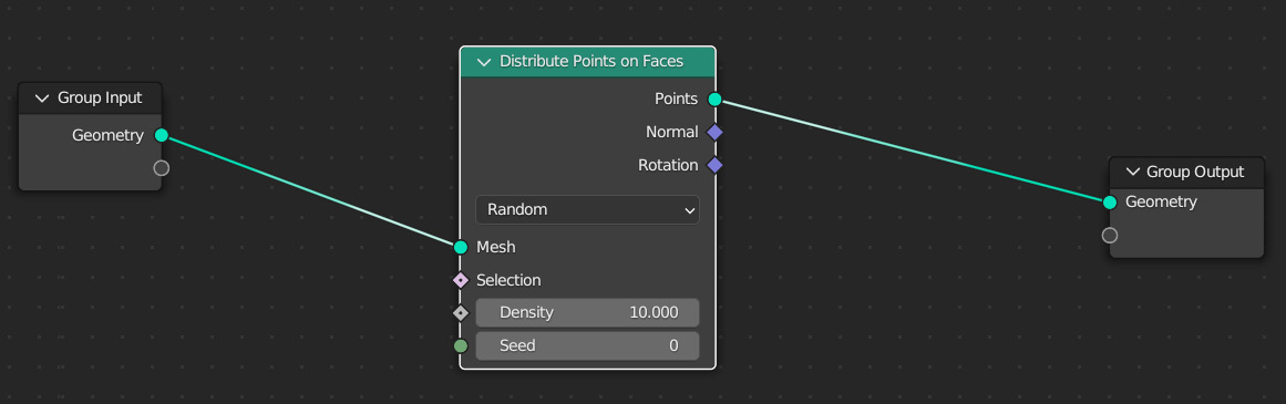
Figure 5.17: Distribute Points on Faces

Geometry Nodes are computed left to right, just like the Material Editor or Compositor that we've used so far. So, we're telling the computer with this node group to take our group input (the landscape object), distribute points on the surface, and then display that in our viewport. Looking at the viewport, you can visualize the points that we're distributing as little orange diamonds:

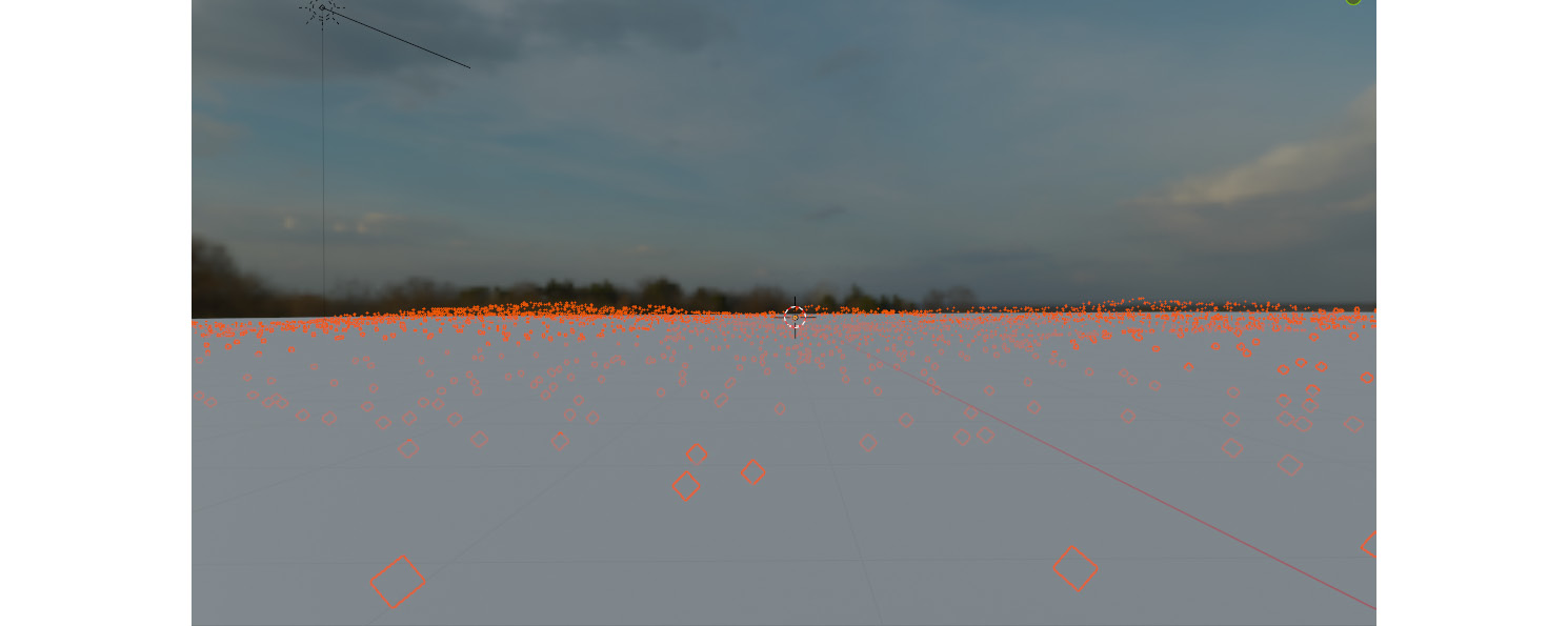
Figure 5.18: Scattered points

5. So, now we need to connect the Grass object to the points we've scattered. Let's do this by adding Instance on Points after Distribute Points on Faces. The Instance on Points node takes each point we scattered with Distribute Points on Faces and adds an instanced object to it. An instanced object can be any mesh we designate:

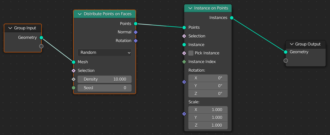
Figure 5.19: Distribute Points on Faces and Instance on Points

6. Then, we need to add an object to distribute. Add an Object Info node and connect it to the Instance input on the Instance on Points node:
   

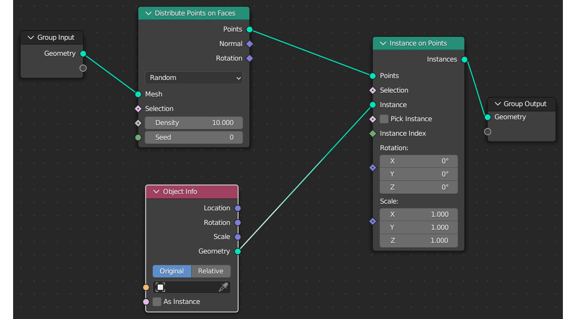
Figure 5.20: Adding the Grass object to the point instance

7. Using the eyedropper on the object box, we can select the Grass object as the object that we want to populate on our landscape:

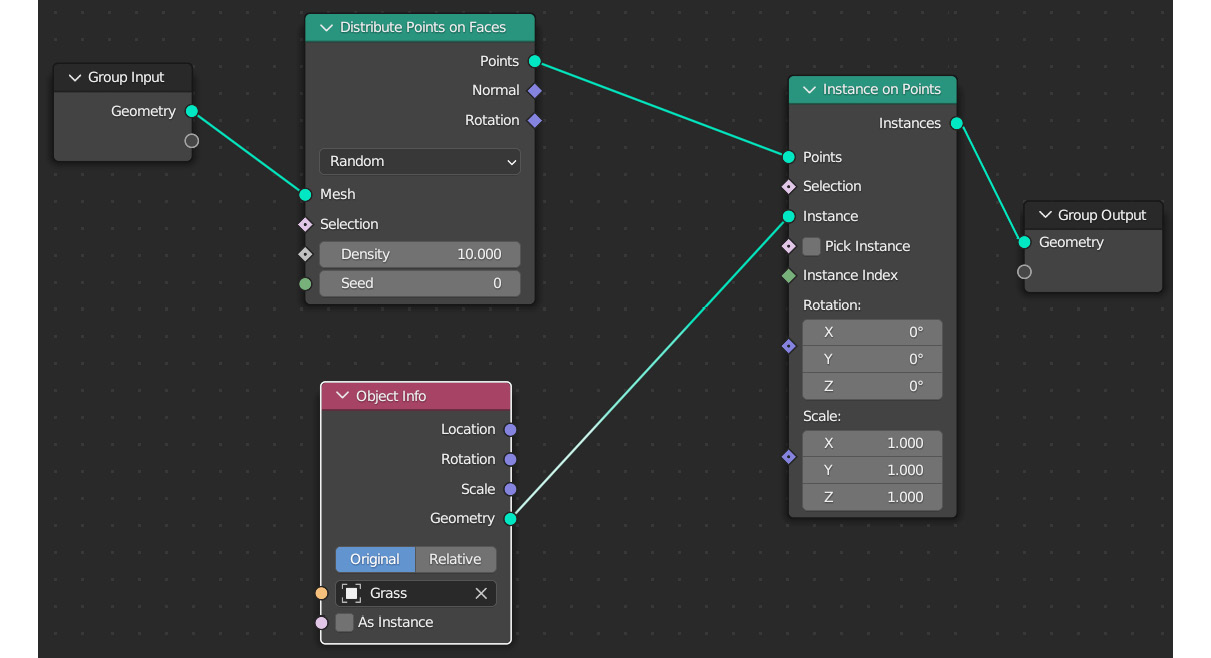
Figure 5.21: Adding the Grass object to the Object Info node

Woah! We have grass suddenly everywhere in the viewport! That isn't exactly what we want, so we'll have to figure out how to make our Grass object a little bit smaller. We can definitely do this by just editing the size of the original object, but I want to show you how to control the size of scattered objects inside of the Geometry Node editor:

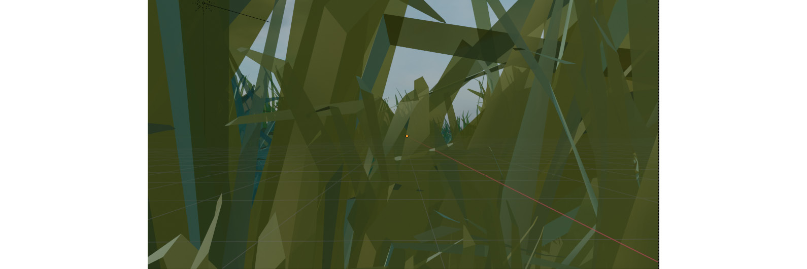
Figure 5.22: The camera view after adding the Grass object to the Instance node

8. We can change the Scale value on the Instance on Points node to 0.100:

Figure 5.23: Changing the point scale

This changes the grass objects to a 10th of their original size, making them decidedly more grass-sized:

Figure 5.24: Grass objects distributed on the foreground landscape object

9. We now have some cool plants to populate our scene. But where did the Foreground Landscape object go? It's completely disappeared in favor of our plants, which isn't what we want. Let's make sure we can see the landscape plane. Add a Join Geometry node and attach it between Instance on Points and the Group Output node. Take the output from the first node, Group Input | Geometry, and connect it to the same input on the Join Geometry node:

Figure 5.25: Joining it all together

We should now see both the landscape and the scattered grass objects together on the screen:

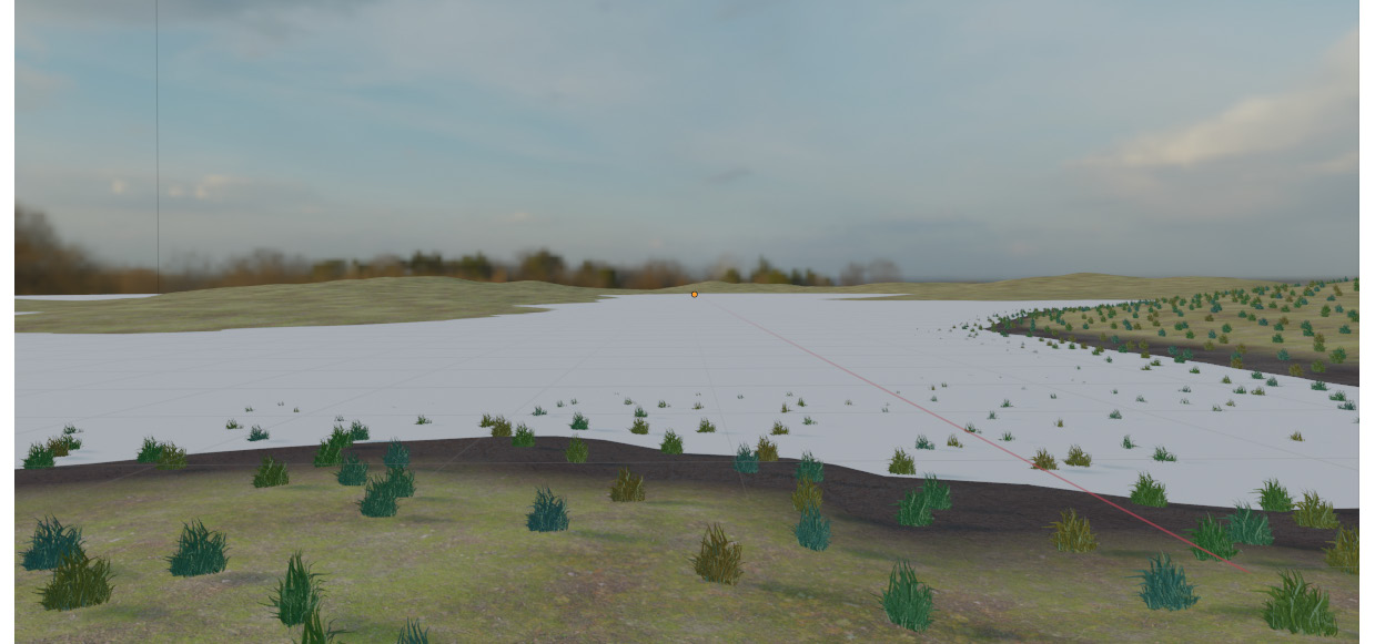
Figure 5.26: The landscape and scattered grass joined together

10. This scattering looks alright, but we probably don't want to have grass appearing underneath the water; it's a waste of computing power. We'll add a Density map now to control where the plants can be scattered. First, we want to connect the empty socket on Group Input to Density on the Distribute Points on Faces node:

Figure 5.27: Adding Density to Group Input

11. Let's go to the Properties menu at the right-hand side of the screen and select the Modifier panel:

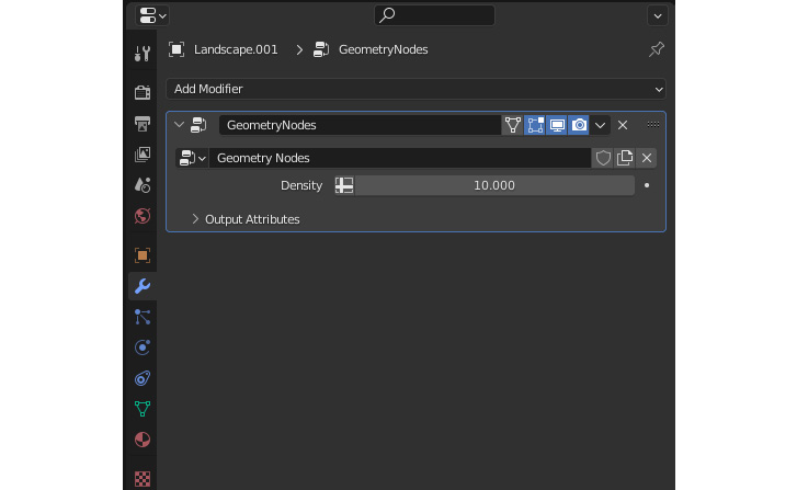
Figure 5.28: The Modifier panel

12. We want to add a vertex group to the landscape, so we'll click on the graph sign next to Density. This should result in the previous number being cleared from the Density value. We can now add a vertex group that we can paint to control the density:

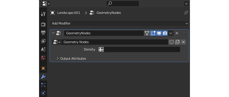
Figure 5.29: Creating a field for the vertex group

13. We need to create the vertex group now. Let's go to Object Data Properties () and add a vertex group using the plus sign on the Vertex Groups section:

Figure 5.30: Creating the vertex group

14. It should give us a vertex group called Group. Going back to the Geometry Nodes modifier, we can now click on the Density field and select Group from the list of options:

Figure 5.31: Selecting the vertex group as the Density field

15. With that vertex group set, we can now change to Weight Paint mode from the drop-down menu at the top-left corner:

Figure 5.32: Weight Paint mode

16. The 3D viewport should now show your landscape as entirely blue. Try painting on top of the landscape with your cursor. The landscape object should change to red (with other shades of yellow and green) as you paint. If this doesn't happen, try changing the Weight and Strength values located at the top left of the screen to 1.000:

Figure 5.33: Weight and Strength toggles

17. In a weight paint map, all red areas indicate where the grass will appear, and all the blue areas indicate where the grass will not appear. I tried to paint all the places that are visible in the camera view red and left anywhere not visible from the camera as the default blue color:

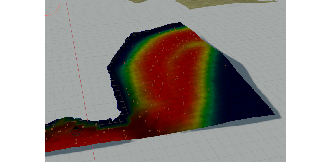
Figure 5.34: Weight painted on the landscape

18. We have plants! If you are still getting grass showing up under the Water Volume object, just jump back into Weight Paint mode and readjust the values so that you get the grass showing up where you want it:

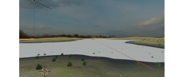
Figure 5.35: Scattered grass after applying the vertex group

19. The last step we'll do in this section is playing with the Density Multiplier. Since this piece of land is close to the camera, we probably want to add more density than, say, the landscape pieces that are farther away from the camera. This way, we can be more efficient, as every grass object has to be calculated by the computer, so if we have four separate pieces of geometry, we can let the background pieces be more sparse, while the foreground pieces are denser. We can change our density by adding a Math node to the Node editor, adding it between Group Input | Density and Distribute Points on Faces | Density:

Figure 5.36: Adding a Math node

20. The default for the Math node is the Add operation. If we click the Add dropdown and switch the operation to Multiply, we can now effectively increase the density of our grass without getting plants under the lake. If you think about it, multiplying by zero is still zero, so therefore, we still have no plants under the water, but we can multiply the amount we're getting on land:

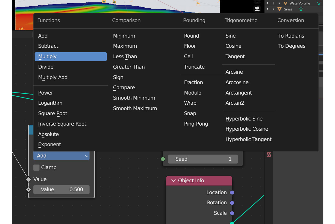
Figure 5.37: Changing the Math node to Multiply

I changed my value to 100.000 and got a result I liked. Feel free to try other values and see how they compare for you:

Figure 5.38: Changing the value to 100.000

After some fiddling with my vertex map, I dialed in my vegetation to create something like the following screenshot:

Figure 5.39: Adding density to the grass scatter

In the next section, we'll add some random variation to the grass objects, add Rocks to the node tree, and then create a reusable system so that anyone can use our system without knowing how to use Geometry Nodes.

Adding more complexity and applying the modifier to other objects

We have an interesting scattering of grass in the scene now. I'm not sure if you noticed, but every single grass object is pointing in the same direction, which isn't very natural. If we want to add randomization to the rotation of the grass, all we need to do is add a randomized value.

Let's get started:

1. Using Shift + A, add a Random Value node and connect it to the Rotation input on the Instance on Points node:

Figure 5.40: The node tree with Random Value added

2. Change the drop-down box from Float to Vector. You may need to reattach the value to the Rotation input after changing to Vector:
   

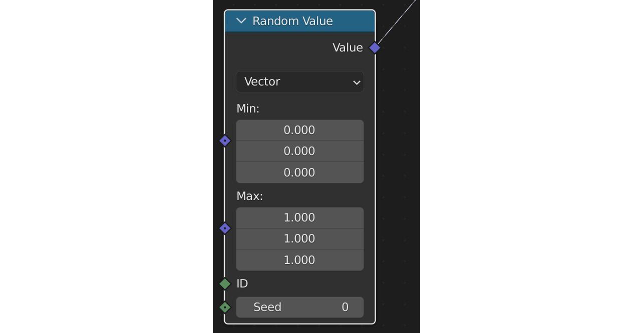
Figure 5.41: Random Value changed to Vector

3. There should be random rotation happening to the grass particles now. But the vector that we designated has three Max inputs and three Min inputs. These inputs are x, y, and z, in that order. So, we have x min, y min, and z min as numbers we can set, as well as x max, y max, and z max, which we can set as well, all from the Random Value node. These numbers are so we can tell the computer the domain in which to randomize. So, for example, if we set the x min to 0.000 and then x max to 1.000, we'll get rotation values between 0.000 and 1.000 for the x axis. So, we can see that the default Random Value setting is to have rotation from 0.000 to 1.000 on all three axes. But we probably only want the grass rotation to be about a 10th of that on two axes (grass doesn't generally grow upside down!). So, if we change the x Max and y Max values to 0.100, we should get a better result:

Figure 5.42: Changes to the max values on the x and y axes

So now, we have some random variation happening in the rotation of our grass objects:

Figure 5.43: Randomly rotated scattered grass

Scale, position, and so on can all be randomized in this way, so try to experiment and see what you can get to work. Try attaching another Random Value node to the scale value and randomize the scale values of the grass as well.

Adding rocks to the node tree

Okay, we've worked in some random variation. Now, let's add our rocks to the node tree. This is where some of the magic happens in the Geometry Nodes process because now that we've got the grass working, we can just copy part of the node network, exchange the grass for rocks, and we'll have an awesome result! Let's get started:

1. Click and drag inside of the Geometry Nodes workspace to select nodes. We want to select Multiply Node, Distribute Points on Faces, Object Info, Random Value, and Instance on Points, so if we click at the top-left corner of the node tree workspace and drag over the nodes we want to select, we should get all of those nodes selected.
2. Use the Ctrl + Shift + D shortcut to copy these nodes while maintaining their connection to Group Input:

Figure 5.44: Copying the nodes

3. In the copied system, we want to delete the Object Info node and replace it with a Collection Info node. Using the Collection Info node, we get the opportunity to add an entire collection to the system, so we can input multiple objects and get several different variations on the object being scattered on the landscape, instead of just the single object:

Figure 5.45: The Collection Info node

4. We need to make a collection with the rocks. Select our two rock objects in the Outliner and use the M shortcut key to open the Collection menu. Select New Collection and then name the collection Rocks. The two rock objects will be moved there:

Figure 5.46: The Move to Collection menu

5. Go back to the Collection Info node and select the new Rock collection in the drop-down menu.
6. Connect the Geometry output on the Collection Info node to the Instance input on the Instance on Points node. Check the Separate Children and Reset Children boxes on the Collection Info node. This means that each rock will be spawned as separate objects, instead of spawning the whole collection at every point:

Figure 5.47: The Collection Info node

7. Connect the whole thing up to the Join Geometry node:

Figure 5.48: The finished node tree

8. You may notice some problems now. There are so many rocks, we can't see any grass. Let's lower the Multiply value of the Rock section of the node tree to something more like 5:

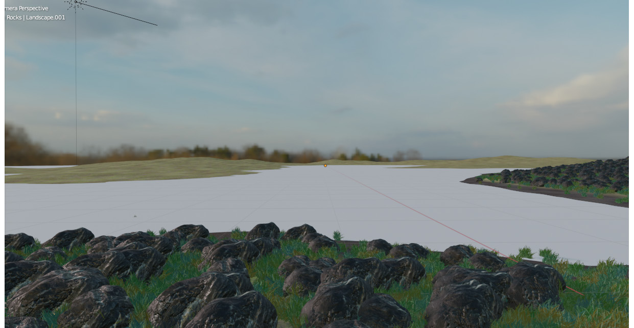
Figure 5.49: Rocks with the density at 5

That's looking pretty good; we have rocks and grass and some really interesting variations that didn't take much time to set up. But you may be asking, why move to Geometry Nodes when we have a perfectly good particle system that we can use just as easily? Well, Geometry Nodes has infinitely more control. It's a steeper learning curve, that's for sure, but it's incredibly powerful. And it can be extremely customizable, with ways to expose values so that you don't even need to look at a Geometry Nodes system if you want to change how many rocks appear in the scene, or their size. Let's add some customizability to our Geometry Nodes system to finish this chapter.

Customizing our Geometry Nodes system

Let's get started:

1. You may have noticed that there was another blank output on the Group Input node, but it's gray. This designates an inactive socket that can be activated, just as we added the Density vertex group. Let's add the value output for the Multiply node on our Grass object to Group Input. Do this by simply grabbing the Multiply | Value socket and dragging it over to hook up with the unused socket on Group Input. The unused socket should now have changed its name to Value:

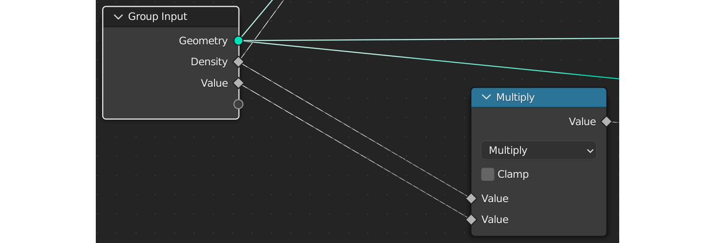
Figure 5.50: Connecting the Density multiplier to Group Input

2. Let's change the name of the socket so we can understand that this is the grass density, not the rock density. Hit N on the keyboard, and the Geometry Nodes menu should fly out on the right side of the panel. You should see Inputs and Outputs listed:

Figure 5.51: Inputs and Outputs in the Group tab of Node options

3. If you click on Value, it should open up a dropdown. Inside the Name box, you can rename it. I'm going to change mine to Grass Density:

Figure 5.52: Renaming to Grass Density

As you can see, the input is renamed so that I can tell what it is. It's possible to add a great variety of customizable inputs to the Group Input node. It allows you to designate what is important to be tweaked and what can be left alone.

4. So, we've added Grass Density as an input, but we need to find where we can edit Grass Density in a simple and convenient way. The place to do this is the Modifier tab! If we click on the Modifier tab (), we can see the Geometry Nodes system that is being applied to this object, with Grass Density labeled and exposed, as with any other value we can change in Blender:

Figure 5.53: The Geometry Nodes modifier with the added Grass Density option

5. We've just created our own custom modifier that anyone can come in and use. Say we're working on a file, and we need to hand it over to a colleague. Well, there's no need to worry that they won't understand our mess of a Geometry Node network. All they need to do is click into the Geometry Nodes modifier we made and tweak values to their heart's content. I added a few more inputs to the Group Input node that I thought would be useful. Simply follow the same procedure I just outlined to add any value to the Input field of the Geometry Nodes modifier:

Figure 5.54: The Geometry Node modifier with more options added

6. The last thing we need to do so that we don't accidentally crash our computer when we reuse this node group is edit the Default values for each input. This way, when we add this Geometry Nodes group, only a few rocks and grass will be scattered. We can then turn up the values that we want. If we leave the default values at 100 every time we add a new modifier, the computer will try to add hundreds of objects instantly and cause our file to crash or severely lag. So, let's select the first Density value and change the default density to 0.000, which is located with the Name and Type options in the Inputs menu:

Figure 5.55: Added inputs to the Inputs menu

Do the same for Grass Density and Rock Density; change them to something small such as 1 or 2.

The other thing we can do that makes Geometry Nodes amazing is apply it to all our other landscape pieces with ease, all with the ability to change anything we want. Let's add some rocks and grass to LeftPlane in our scene:

1. Select LeftPlane in the scene.
2. Go to Weight Paint mode and paint a Density map for the left plane.
3. Go to the Modifier tab, select the Add Modifier dropdown, and select the Geometry Nodes option. This adds a new Geometry Nodes modifier, not the one we just worked on. So, we need to link the old node tree to this new modifier.
4. Select the Browse Node Tree to be linked button (it looks like two little nodes connected by a line, next to the Geometry Nodes name):

Figure 5.56: Browsing to another Geometry Nodes tree

5. Select the first entry, the original Geometry Node network we just made. Feel free to rename it if it helps you to keep organized:

Figure 5.57: Changing the Geometry Nodes tree dropdown

6. We should now see the rocks and grass appearing on the left plane. Change the Density map to the one we just painted for this land object using the same method we did for the first landscape object. Try increasing Grass Density or Rock Scale, and see how it affects the objects scattered on the left plane but not the objects on the plane closest to us:

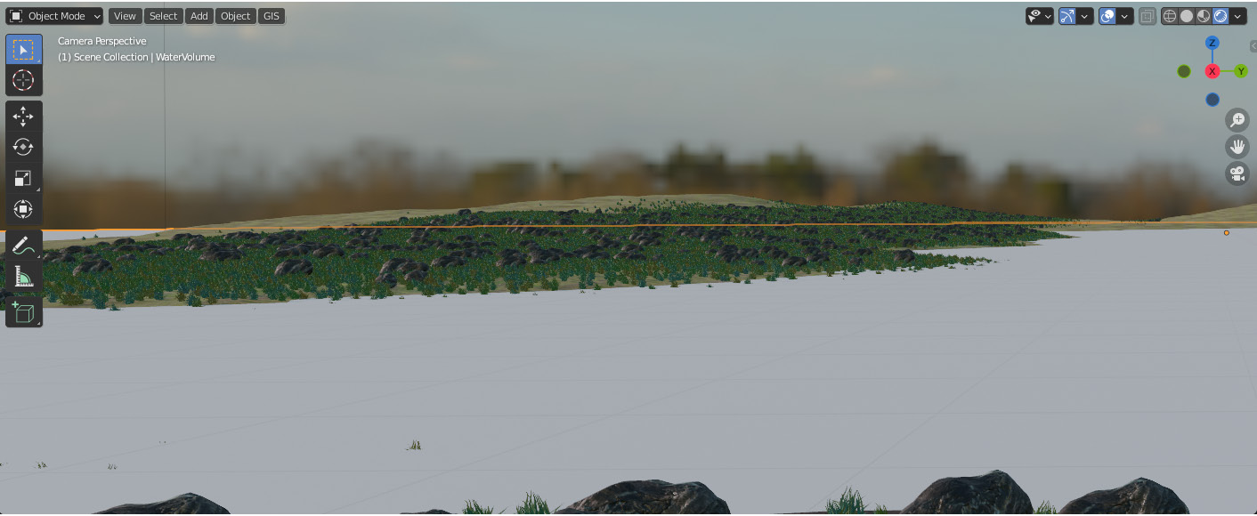
Figure 5.58: The same node tree being applied to the background object

Projecting all these objects is pretty hard on the computer, so try to only work on one plane at a time, disabling the Geometry Nodes modifier on planes that you're not working on as you focus on others. This is why the landscape is broken up into pieces – so that we can work on the foreground and background at separate points in time, and not have the whole scene full of plants trying to show in the viewport all at one time. EEVEE is good, but it's not that good!

Summary

I hope you are as excited as I am about this new step in Blender's development program. Geometry Nodes provides an artist with infinite variation, customization, and adaptability. It's also faster in the long run; next time you want to scatter objects on another plane, all you have to do is import the network and tweak it as needed. We've just scratched the surface on what is possible with this amazing tool, and I hope you feel motivated after looking at this simple introduction to the subject to learn more. We just created an amazing node network that scatters grass, rocks, or anything on a landscape; then, we learned how to add random rotation and control the size of the grass and rocks directly inside of the Geometry Node network. Then, we customized our network so that we can reuse it over and over again, without needing to create copies or fake users to change the values.

That's all we'll do with Geometry Nodes for this project. In the next chapter, we're going to make a shader for the water and then learn about how to add reflections so that we get an accurate reflection of the sky and the surrounding environment, making our scene look more realistic.