Chapter 4: Non-Physical Rendering

The last chapter ended with us applying some of the finishing touches to our materials, modeling, effects, lighting, camera, and design. But in 3D animation, and especially with EEVEE, that isn't enough to consider a piece of art "finished." As you know, we have to render! And rendering can sometimes be the trickiest part of the equation that is a scene. If you've worked with EEVEE before inside of Blender, you know how frustrating it can be to make EEVEE do what you want. There's so much to know and understand about how EEVEE works that when it comes to rendering, it can seem overwhelming. That's why we're starting with a non-physically rendered scene so that we can start to understand how to use some of the tools the Blender developers have given us and start to feel more comfortable setting up EEVEE for success. In Sections 2 and 3 of this book, we'll go over more techniques in the rendering stage, so don't feel too bad if you still have questions after this part; we'll get to them, I promise! For now, we'll look at a few things:

• Adding clouds to our composition
• Configuring Render settings
• Using layers to combine elements in the compositor

Technical requirements

In this chapter you again have two options – download my prepared and completed file with all my assets, materials, lights, and cameras, or use your own that you created. We'll be finishing off the scene and then rendering it out, so make sure you're working on a computer with a GPU with the best specs that you can muster. Rendering is the most time-intensive and computationally expensive part of the animation process, so plan accordingly. Even if you don't have an amazing computer, EEVEE is obviously a lot less intensive than Cycles, so don't worry if you're trying to work on a laptop or an old computer. It's just better to work with the best you have for this chapter. The other file you might want for this chapter is named MiniProject1_Compositing.blend, and will be used in the final compositing section.

The sample files used in this chapter are available here:

https://github.com/PacktPublishing/Shading-Lighting-and-Rendering-with-Blenders-EEVEE/tree/main/Chapter04

Adding clouds to our composition

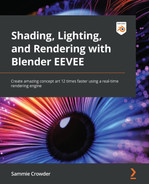
We've created a cool house with some fun features, but, we can still see the empty space around the house, which doesn't really lend itself to a good composition. Let's fix this right now. The reason we've waited until the very end to add the clouds to our scene is that the volumetric shader we'll be using requires tweaking the Render settings, so it doesn't make much sense to create clouds until we're ready to render. We're starting from the file I have set up, which looks something like this at the start:

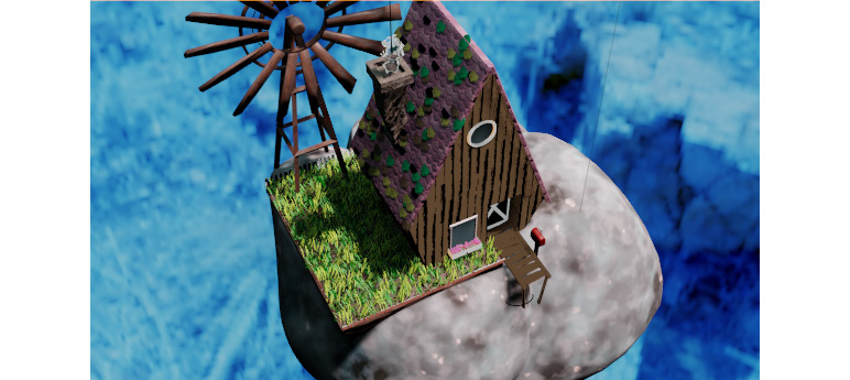
Figure 4.1: Starting image

I'm looking from the camera view and all my lights, materials, and background are set up. The house looks good, but we probably don't want that blue surrounding space; it doesn't look good! Let's add some clouds to fix it:

1. Add a cube to the scene, using Shift + A, and select the Cube object.
2. Give it a new material and delete the Principled shader that comes by default.
3. Add a Principled Volume node and plug it into the Volume input under Material Output.

Figure 4.2: Principled Volume shader

4. Let's try an experiment to show how Principled Volume works inside EEVEE because it doesn't work as expected. If we go to the cube we added the Principled Volume shader to and edit it, you can see that the Principled Volume shader doesn't actually change with the geometry shape. The Principled Volume shader in EEVEE can only be rendered in a cube shape! So we can't model some cloud geometry and just have clouds work; we need to apply some shader magic.

Figure 4.3: Volume shader only rendering in cubic form

5. Undo the previous edit (Ctrl + Z) and come back into the shading workspace. Add a Texture Coordinate node, a Mapping node, and a Gradient Texture node, with the dropdown changed to Spherical. Set them up as in the following screenshot:

Figure 4.4: Mapping node

6. Then, use the Ctrl + Shift shortcut and click on the Gradient node to preview the Gradient Texture node in the viewport. You might not see the result instantly (I have to rotate my cube around to see the Gradient Texture node being projected on it).

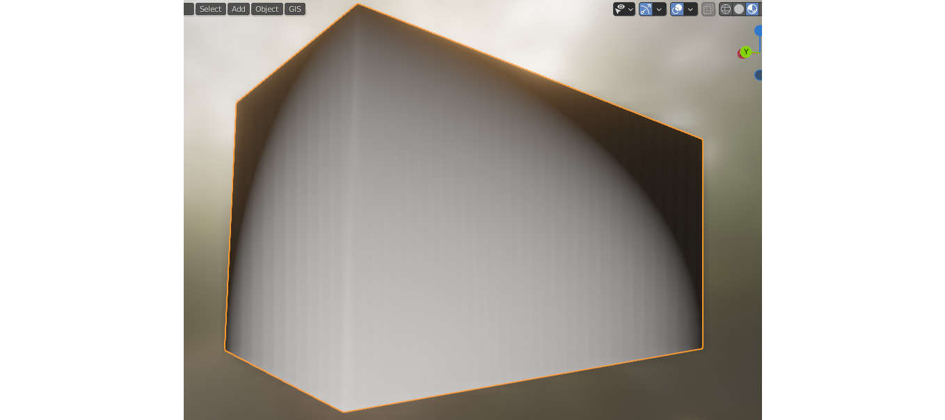
Figure 4.5: Gradient Texture default

7. I tweaked a lot of my values in the Mapping node to make Gradient cover my cube how I wanted. These are the values I ended up with, but experiment and see what you prefer:

Figure 4.6: Mapping node with changes

When we preview Gradient Texture with the new mapping, you should have something like this on your cube:

Figure 4.7: Gradient with mapping changes

8. Next, we'll add Noise Texture and a MixRGB node.

Figure 4.8: Adding MixRGB and Noise Texture

9. Put the output of Gradient Texture into the top Color input of the Mix node and the Fac output of Noise Texture into the input of the bottom Color socket of the Mix node. Change the Blending mode of the Mix node to Multiply, change Fac to 1, and then use our shortcut of Ctrl + Shift + Click on the Mix node to preview it.

Figure 4.9: Mixing with Noise Texture

Node Wrangler Preview

Node Wrangler is an amazing add-on (especially since it's free!), and one of its most amazing pieces of functionality is the ability to preview any node in the viewport by just pressing Ctrl + Shift and clicking on the node you want to preview. Try it out. It's very useful to be able to preview a specific part of your shader without having to wonder whether you're tweaking the right value.

10. Next, we'll add a color ramp to the output of the Mix node. This creates a gradient of color that we can change by moving the color sliders on the left and right.

Figure 4.10: Adding a color ramp

11. I changed the white color on the right to a more grayish color and then pulled the right slider over almost next to the left slider.

Figure 4.11: Adding a color ramp

My preview of the color ramp now looks like this in the viewport.

Figure 4.12: Noise and Gradient Texture output

12. So now that we've sketched out the rough outline of a cloud on our cube, all we have to do is use it to create the volumetric appearance of clouds. How we'll do this is a decidedly non-physically-based method, so applying this exact procedure to a photoreal scene is not advisable. We'll cover that in the next two projects. Let's take the Color output from the color ramp and input it into Density of our Principled Volume shader, the Emission Strength input, and the Emission Color input. So, anywhere our incoming texture is black is going to be see-through, and anywhere we have white is going to be "cloud."

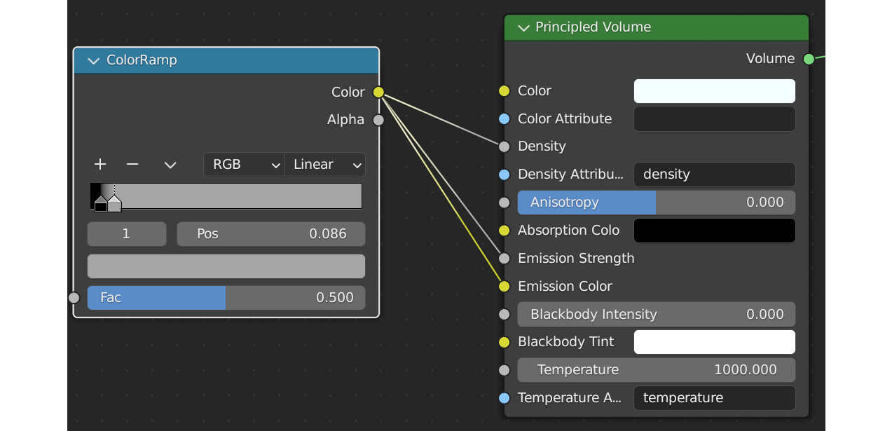
Figure 4.13: Principled Volume with inputs

13. Mine came out something like this. You can tweak the color ramp to make the cloud bigger or smaller or change the scale of Noise Texture to refine the raggedness of the edges. As you can see though, from the right angle it looks pretty cloud-like! Of course, if you turn the cube to look at it from another direction, the effect isn't so good, but right now we're only looking at it from one camera angle, so we won't worry about potentially seeing a cloud's "edge":

Figure 4.14: Result of Principled Shader with inputs

14. I duplicated my one cloud a few times and placed each cloud by hand, making each individual cloud bigger or smaller and rotating the cloud to get a different view of it from the camera. I ended up with something like this:

Figure 4.15: Result with clouds

15. I decided these clouds were a little too dark, so I went back into the shader, added another color ramp, and then tweaked the colors until they were more like what I wanted and plugged that into the Emission Color input.

Figure 4.16: Adding more color with another color ramp

I liked the more ambient nature of the clouds when they had some blue mixed into them and I think this worked better with the overall vibe we already created in Chapter 2, Creating Materials Fast with EEVEE, and Chapter 3, Lights, Camera....

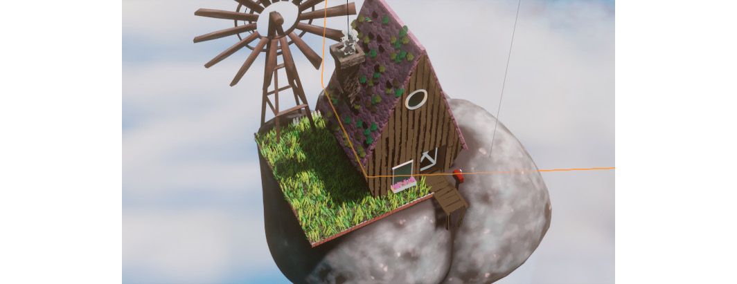
Figure 4.17: Finished clouds

16. The final stage in making our clouds look perfect involves going into the Render settings, which is why we waited until now to create the clouds. If you go to the right-hand properties panel, you'll see the Render Properties panel is the little camera at the top. Click on that, navigate down to the Volumetrics section, and then click the twirl-down arrow to open the Volumetrics options.

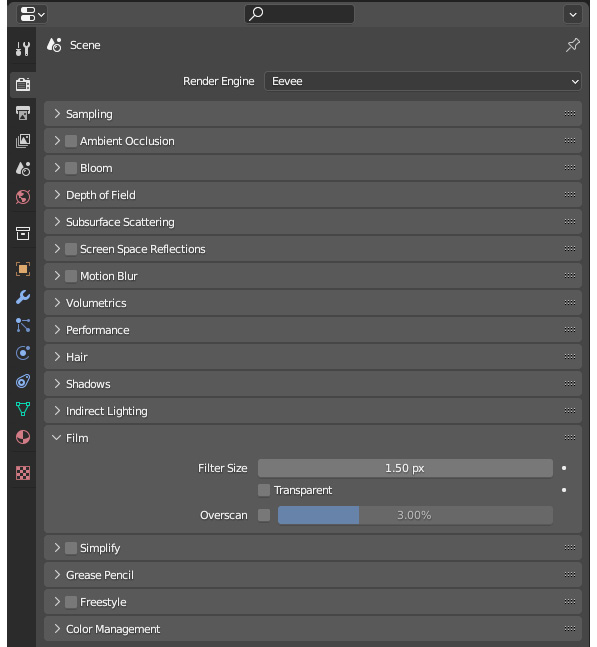
Figure 4.18: EEVEE Render panel

17. There are a number of options, most of which we'll change here. First, change the Start value to 15 m and the End value to 95 m. These values tell EEVEE when to start and end the volumetric zone, so EEVEE isn't rendering volumetrics that fall outside of the camera area. Following that idea, these values are based on where my camera and my clouds are, so try lowering them. The closer these numbers are together, the less volumetric rendering happens in the final render and the less computational power we'll use, so getting the optimized value for those is necessary.
18. Tile Size is the size of the pixel chunks used to render the volumetrics. The smaller the number, the better the resolution. I'm going to stick to 16 px in this case, but if your computer can stand it, try using a smaller value.
19. The Samples value is just what it seem like it might be: the number of samples used to render the volumetrics. Try to stick to numbers compatible with a 64-bit system, such as 16, 64, 128, and 1,024. I think 128 samples is plenty to compute the clouds we have here without too many problems.
20. The Distribution value is the level of blending between exponential and linear sample distribution. Put simply, this means that sections closer to the camera will have more samples than sections further away from the camera. It's not something I find myself tweaking that often, so if you don't feel like you understand what this value does, just leave it at the default. I left my value on 0.8.
21. Check the boxes next to Volumetric Lighting and Volumetric Shadows. Samples under Volumetric Shadows can be useful to tweak if your computer is having trouble rendering, but I left mine at 16.

Figure 4.19: Volumetrics options in the Render panel

And there you go! We have some cool clouds that utilize the Volumetrics feature of EEVEE and we managed to get a cloud-like shape, even though EEVEE can't create volumetric geometry in any way other than cubic. We'll explore other methods for creating volumetric effects later on in the book, but I think this is a great technique for creating quick and dirty clouds that can be used in a variety of situations to break up the sky a little bit and add depth.

Figure 4.20: After configuring volumetrics

We also dipped our toes into the Render Properties panel, something that we'll continue to explore in the next section.

Configuring Render settings

The Render settings of any scene can take a finished product from mediocre to top-notch. Hopefully, you'll have some experience with Render settings from previous projects in Cycles, but in EEVEE, the importance of the Render settings becomes even greater. This is because, in a rasterized real-time renderer, a lot of the settings that really make a scene pop are at the default setting of off. So we, as artists, need to know which settings to use to make sure we get the most out of EEVEE, but also which ones to skip in order to maintain as much efficiency as we can.

Let's look at the options in order, explaining how each affects our render with examples. The Render Properties panel contains all the Render settings that we'll be looking at for now. The Render Properties panel should be on the right-hand side of the screen in the Properties editor. Select the Camera icon if you don't see the Render settings in your Editor panel.

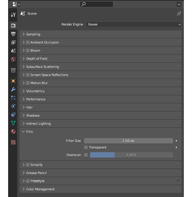
Figure 4.21: Render panel (redux)

Let's go through each setting that pertains to our current scene. In this chapter, we'll be looking at the Sampling, Ambient Occlusion, Bloom, and Screen Space Reflections sections. If we skip something, assume that it doesn't have any bearing on our current scene.

Sampling

Sampling is a measure of how many samples the rendering engine will take in one frame. A sample is one calculation of how the lighting is bouncing around the scene. So, if we have more samples, we're bouncing more light around the scene and getting a more accurate output of what the scene actually looks like. Since we're using EEVEE and not Cycles, our samples are actually calculating the approximate behavior of the light so that we can view our scene faster.

Figure 4.22: Sampling options

So, it follows, the more samples, the more refined our final output will be. But more samples also equals a longer render time. So, we need to dial in our Render number so we don't wait too long for the render, but we also get a good final product. The Viewport number in this section is the number of samples from the viewport. I find the best way to decide how many samples you might need is by testing it out in the viewport. Right now, we have 16 samples in the viewport, which is looking pretty good in my output preview. I'm going to push my Render sample number to 128 (following the rule of 8-bit numbers), just because I think we can afford more samples with how fast 16 samples are rendering.

This is really a trial-and-error stage, which will get easier as you get more experience. So, try out some numbers and render them and see how things turn out. Luckily, EEVEE is lightning fast and you really won't have to wait too long until you want something insane, such as a million samples.

Ambient Occlusion

Ambient Occlusion is a really useful thing in 3D. It pretty much means that where two meshes are close together, shadows will be added. This mimics what happens in real life, where two objects will throw shadows on each other that get deeper when the objects get closer. Ambient Occlusion is a setting inside of EEVEE that defaults to off, so we need to turn it on by clicking the box next to Ambient Occlusion.

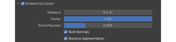
Figure 4.23: Ambient Occlusion options

I find most often that Distance is the only number I end up playing with. If I want a more pronounced ambient occlusion, I'll pump that number up to 1 m.

Figure 4.24: Before ambient occlusion

Now we'll look at the effect ambient occlusion has on the scene.

Figure 4.25: After ambient occlusion

As you can see, the areas where the two rocks overlap are now more shadowed, and we have more definition on the shadow of the house.

Bloom

Let's turn Bloom on as well by clicking on the checkbox for Bloom. Bloom has to do with the lighting in the scene. It simulates a light bleed effect from the lights we have and gives the whole scene a softer look.

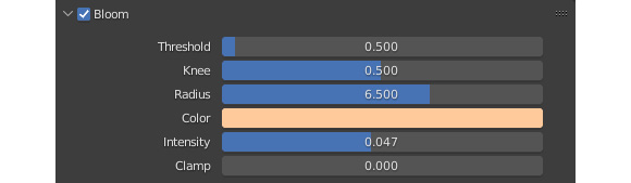
Figure 4.26: Bloom options

Changing the value of the Threshold setting is most useful. A higher threshold means less bloom, while a lower threshold means more bloom. It's subtle, but a very low number such as 0.2 definitely gives it a hazy look that a higher number such as 1 will not.

Figure 4.27: Before Bloom

And now let's see how Bloom has changed what we see in the viewport:

Figure 4.28: After Bloom

The other thing I like to play with is the color of the bloom. The overall look really changes if you input a cold color, such as blue, instead of a warm color, such as orange, that we had as the default.

Figure 4.29: Green bloom

I kept a light orange color as the final color of my bloom and kept the threshold at 0.3. This is a stylized rendering, so having a little more bloom will help us to achieve that style, but in a more realistic scene, we would probably not want to have so much bloom. We'll look at bloom a lot more in the third mini-project, in Chapter 9, Lighting an Interior Scene, as a way to get specific lights to pop.

Screen Space Reflections

Turning on Screen Space Reflections will just change one small thing in our scene: the windows.

Figure 4.30: Screen Space Reflections options

Screen Space Reflections makes any surface that is above a certain threshold of reflectivity reflect light. It's a complicated notion, one that we'll talk a lot more about in Chapter 7, Faking Camera Effects for Better Renders, when we create a whole lake of water that we'll need to be reflective.

Figure 4.31: Before Screen Space Reflections

Now look at the Screen Space Reflections addition, with refraction on:

Figure 4.32: After Screen Space Reflections

Pretty subtle huh? From this angle, we can only see the way the window is now reflecting the flower box. This isn't a truly significant difference at the moment. We can increase the window's ability to reflect at this angle by unchecking the Refraction setting. This is not physically correct, so in more realistic scenes, we would absolutely want to keep refraction on, but in this case, where we're exercising more artistic control, I like a little more reflection on the window.

Figure 4.33: After turning off refraction

Film

The last setting we need to check is the Film Transparent option.

Figure 4.34: Film options

This will make the background of our scene transparent, so we can render out a good alpha channel to work with in our compositing system.

At this point, we've made all the changes we need to the settings. Let's now set ourselves up to render and composite a really cool finished piece.

Compositing Render layers

That's the extent of what we'll cover in terms of the Render panel for this project, but more will be covered in future chapters of this book, where we'll get deep into baking and other EEVEE features. At this point, we have two separate features that are going to be composited together to create something really cool. If you remember from the previous chapter, we made some line art to add some lines to the outer edges of the geometry in the models to get more of a comic book feel. Let's add those back into our preview by unhiding them from the Render view. So this looks pretty cool, as is, but if we want to take it one step further and render the clouds and the geometry of the scene separately, it will give us a lot more flexibility in the final composite. Feel free to start this section from your own work that you've done in previous chapters, or download my prepared .blend file from GitHub, named MiniProject1_Compositing.blend.

Figure 4.35: Starting the compositing

To start our composition we need to go to the outliner and create another View Layer.

x

Figure 4.36: Creating a new View Layer

View Layers are ways in which we can render certain parts of our scene so that we can combine them in interesting and creative ways. We'll use View Layers to separate the clouds from the house and then recombine them later:

1. Hit New in the menu options and that should add a new View Layer to our scene.
2. Click on the title of the View Layer to rename it to Clouds.
3. Next, uncheck every collection in the scene except for Clouds and the Lighting collection.

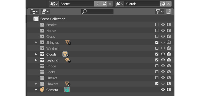
Figure 4.37: The Clouds layer

This deactivates them from the render of this scene, so we will only render out Clouds in this View Layer.

Figure 4.38: Result of the Clouds layer

4. Next, go back up to the top right and change the active View Layer back to the default View Layer with the drop-down menu button.
5. Then, go to the collection where we're holding all the clouds.
6. Click the checkmark on the right that corresponds with Clouds to deactivate it from the default View Layer.

Figure 4.39: The collections visible in the default View Layer

Notice that when we deactivate the clouds from the default View Layer, they no longer appear in the render.

Figure 4.40: The default View Layer result

Now we've set up the right View Layers, let's select the Compositing workspace from the workspace tabs at the top of the screen.

Figure 4.41: The Compositing workspace

7. Enable the compositing nodes by selecting the checkbox called Use Nodes in the top menu area.

Figure 4.42: Use Nodes option

8. You should see the nodes open up in the workspace. We want to select the Render Layers node and copy it with Shift + D.

Figure 4.43: Duplicating the render layers

9. Change the View Layer for the second render layer to the cloud layer we made.

Figure 4.44: Render layers with the Clouds option selection

10. Next, we'll add three File Output nodes (with the Add menu accessed from our usual shortcut, Shift + A).
11. Attach the Image output to the Image input of File Output and select a path for your image to be saved out to. There should still be one File Output node available to attach an input to. We need to render out an environment pass so that we can put the background into our composite.

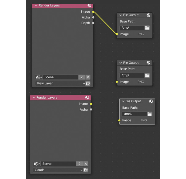
Figure 4.45: Adding more file outputs

12. Let's now go to the View Layer properties, which is inside the Properties panel (on the right side of the screen) and looks like a little picture.

Figure 4.46: The Passes options

13. Make sure you've selected the first View Layer (not the clouds). Check that the Combined and Z passes are selected, as Line Art Modifier needs this information to render out properly. Then, select the Environment pass in the Light category. We'll revisit passes in more depth later in the book.
14. Take the output of the environment in the first View Layer and put it into the third File Output image input.

Figure 4.47: Adding the Environment pass

15. The shortcut to render is F12. Let's give it a whirl!

I now have three separate passes – the default View Layer, the cloud View Layer, and the environment. These images can now be combined any way we want. If you like Photoshop or Krita, you can use those to combine these three passes, or if you want to stay in Blender, we have the option to combine those three images natively in our compositor. I'll show you the Blender way, but you should do what is comfortable for you.

Side Note

If you want to use Krita (another awesome open source program), they have great documentation to get you started on compositing in their program: https://docs.krita.org/en/user_manual/getting_started/basic_concepts.html.

Final compositing

We're on the home stretch! In this final section, we'll look at how to add the two images we rendered out together inside Blender so that you can see how powerful the use of separate passes is. Let's get started:

1. I like to open a new fresh Blender window to composite, just in case I still need to make tweaks to the original render. This way, we can save our Mini-Project 1 file as is and come back to it later if we want to add or remove something.
2. Let's go to the Compositing tab again and select Use nodes (again).
3. Import the three images we rendered out. I like to drag and drop them from the File folder into the compositing window, but you can also use Add and select Image and import them with File Manager.

Figure 4.48: Starting the final compositing

4. Hit the N key to pull up the Backdrop option. Check the box that says Backdrop and click on the Fit option once. This inputs the viewer output into the background of our scene so we can see what we're doing as we work. Use the Node Wrangler add-on shortcut, Ctrl + Shift + Click, to preview a specific node.

Figure 4.49: Turning on Backdrop in the compositor

5. Add two Alpha Over nodes to the compositor.
6. Put the environment pass into the top of the first Alpha Over Image input, and the cloud pass into the second Alpha Over Image input. Then, take the second Alpha Over node and do the same with the output of Cloud and Environment combined and the house pass.

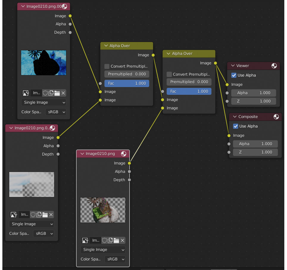
Figure 4.50: Using the Alpha Over nodes to connect

Now we have pretty much recreated the original render. Why did we go through the trouble of rendering three separate passes to create the exact same thing as we had at the beginning?

Well, the magic of compositing is the ability to tweak parts separately. Let's put a Hue Saturation Value node in between the Cloud pass and the first Alpha Over node.

Figure 4.51: Using the Hue and Saturation nodes to change the render

If we change the values of Hue Saturation Value, we can affect just the clouds. Or, if we incorporate an RGB curve in between the House pass and the second Alpha Out node, we can change the color of just the house, making it a little bluer. We can also change the factors of the Alpha Over nodes to show more or less sky, make the clouds more obvious; basically, we can do anything we want!

Figure 4.52: Tweaking our layers

After playing with some values and making some small tweaks, I ended up using a Hue Saturation Value node on the house to make it more richly colored and cartoony, and then used RGB curves on the clouds and sky to tweak them until I liked how it was all blending together. I added another File Output node and then pressed Render again. Here's how my finished product looks:

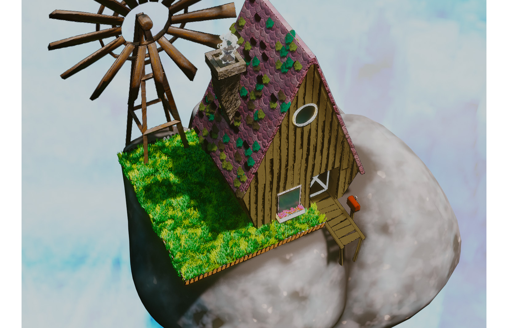
Figure 4.53: The final render

The huge advantage of rendering out passes is worth the little extra time to set them up. Imagine your boss, the art director, comes to you saying she wants this finished product to look a little more green, and the background a little less bright. All you need to do is go back to the composite, tweak two values, and save it out again. If you hadn't saved each layer separately, you'd have to go all the way back to the original file and change the lighting or materials or any number of time-consuming things to get the right look for the shot. So, don't discount the practice of being organized and planning for future changes.

Summary

I really hope you enjoyed working through this process of our first mini-project. I think we ended up with a really cool stylized scene that laid down some of the fundamental practices of working with EEVEE. We created materials, lights, effects, and more to pull this really fun, simple scene together. A lot of the components we touched on in this chapter will be important in the next mini-project, so go over some of these workflows, use them to create other projects, and make sure you feel confident in working with EEVEE before you move on to the next mini-project, which will involve creating an environment landscape, complete with trees, grass, and water.

In the next chapter, we will go over Geometry Nodes, an amazing, powerful new feature in Blender, and see how we can use them to create grass, rock, and tree distributions.