Chapter 9
Volume Controls
A volume control is the most essential knob on a preamplifier – in fact the unhappily named ‘passive preamplifiers’ usually consist of nothing else but a volume control and an input selector switch. Volume controls in one guise or another are also freely distributed on the control surfaces of mixing consoles, examples being the auxiliary sends and the faders.
A volume control for a hi-fi preamplifier needs to cover at least a 50 dB range, with a reasonable approach to a logarithmic (i.e. linear-in-dB) law, and have a channel balance that is better than ±1 dB over this range if noticeable stereo image shift is to be avoided.
The simplest volume control is a potentiometer. These components, which are invariably called ‘pots’ in practice, come with various control laws, such as linear, logarithmic, anti-logarithmic, and so on. The control law is still sometimes called the ‘taper’, which is a historical reference to when the resistance element was actually physically tapered, so the rate of change of resistance from track-end to wiper could be different at different angular settings. Pots are no longer made this way, but the term has stuck around. An ‘audio-taper’ pot usually refers to a logarithmic type intended as a volume control.
All simple volume controls have the highest output impedance at the wiper at the −6 dB setting. For a linear pot this is when the control is rotated halfway towards the maximum, at the 12 o’clock position. For a log pot it will be at a higher setting, around three o’clock. The maximum impedance is significant because it usually sets the worst-case noise performance of the following amplification stage. The resistance value of a volume control should be as low as possible, given the loading/distortion characteristics of the stage driving it. This is sometimes called ‘low-impedance design’. Lower resistances mean:
less Johnson noise from the track resistance;
less noise from the current-noise component of the following stage;
less likelihood of capacitive crosstalk from neighboring circuitry;
less likelihood of hum and noise pickup.
A linear pot is a simple thing – the output is proportional to the angular control setting, and this is usually pretty accurate, depending only on the integrity of the mechanical construction. Linear pots are given the code letter ‘B’ (see Table 9.1 for more code letters).
Table 9.1 Pot law identification letters
ALPS code letter |
Pot characteristic |
|---|---|
A |
Logarithmic |
B |
Linear |
C |
Anti-logarithmic |
RD |
Reverse log |
Log controls are rather less satisfactory. A typical log pot is not a precision attenuator with a fixed number of dB attenuation for each 10 degrees of shaft rotation. It is instead made up of two linear slopes that roughly approximate a logarithmic law, produced by superimposing two sections of track made with different resistivity material, the overlap usually being at the bottom end of the control setting, such as 20% of full rotation (see Figure 9.1). These pots are usually given the code letter ‘A’.

Figure 9.1: The control laws of typical linear and log pots
Anti-logarithmic pots are the same only constructed backwards, so that the slope change is at the top end of the control setting; these are typically used as gain controls for amplifying stages rather than as volume controls. These pots are usually given the code letter ‘C’.
There is a more extreme version of the anti-logarithmic law where the slope change occurs at 10% of rotation instead of 20%. These pots are useful where you want to control the gain of an amplifying stage over a wide range, and still have something like a linear-in-dB control law. Typically they are used to set the gain of microphone input amplifiers, which can have a gain range of 50 dB or more. These pots are given the code ‘RD’, which stands for reverse D law; I don’t think I have ever come across a non-reverse D law. Some typical laws are shown in Figure 9.1.
Please note that the code letters are not adhered to quite as consistently across the world as one might hope. The codes given in Table 9.1 are those used by ALPS, one of the major pot makers, but other people use quite different allocations; for example Radiohm, another major manufacturer, calls linear pots A and log pots B, but they agree that anti-log pots should be called C. Radiohm have several other laws called F, T, S, and X; for example, S is a symmetrical law apparently intended for use in balance controls. It clearly pays to check very carefully what system the manufacturer uses when you’re ordering parts.
The closeness of approach to an ideal logarithmic law is not really the most important characteristic of a volume control. Of greater importance is the matching between the two halves of a stereo volume control. It is common for the channel balance of log pots to deteriorate quite markedly at low volume settings, causing the stereo image to shift as the volume is altered. You may take it from me that customers really do complain about this, and a good deal of ingenuity has been applied in attempts to extract good performance from indifferent components.
An important point in the design of volume controls is that their offness – the amount of signal that gets through when the control is at its minimum – is not very critical. This is in glaring contrast to a level control such as an auxiliary send on a mixer channel (see Chapter 17), where the maximum possible offness is very important indeed. A standard log pot will usually have an offness of the order of −90 dB with respect to fully up, and this is quite enough to render even a powerful hi-fi system effectively silent.
Loaded Linear Pots
Since ordinary log pots are not very accurate, many other ways of getting a log law have been tried. An approximation to a logarithmic law can be made by loading the wiper of a linear pot with a fixed resistor R1 to ground, as shown in Figure 9.2. Trace 1 in Figure 9.3 (for a linear pot with no loading) makes it clear that the use of an unmodified linear law for volume control really is not viable; the attenuation is all cramped up at the bottom end.

Figure 9.2: Resistive loading of a linear pot to approximate a logarithmic law

Figure 9.3: Resistive loading of a linear pot: the control laws plotted
Adding a loading resistor much improves the law, but the drawback is that this technique really only works for a limited range of attenuation – in fact it only works well if you are looking for a control that varies from around 0 to −20 dB. It is therefore suitable for power amp level controls and aux master gain controls (see Chapter 17 for details of the latter) but is unlikely to be useful for a preamplifier gain control, which needs a much wider logarithmic range. Figure 9.3 shows how the law varies as the value of the loading resistor is changed, and it is pretty clear that whatever its value, the slope of the control law around the middle range is only suitable for emulating the ideal log law labeled ‘20’. The value of the loading resistor for each trace number is given in Table 9.2.
Table 9.2 The loading resistor values used in Figure 9.3
Trace number |
Loading resistor R1 value |
|---|---|
1 |
None |
2 |
4k7 |
3 |
2k2 |
4 |
1 kΩ |
Figure 9.3 shows that with the optimal loading value (trace 2) the error in emulating a 0 to −20 dB log range is very small, lying within ±0.5 dB over the range 0 to −16 dB; below this the error grows rapidly. This error for trace 2 only is shown in Figure 9.4. Obtaining this accuracy naturally relies on having the right ratio between the pot track resistance and the loading resistor. The resistance of pot tracks is not controlled as closely as for fixed resistors, their tolerance usually being specified as ±20%, so this does present a significant problem. The only solution is to make the loading resistor trimmable, and this approach has been used by at least one console manufacturer.

Figure 9.4: Resistive loading of a linear pot: the deviation from an ideal 20 dB log law
Another snag to this approach is that when the control is fully up, the loading resistor is placed directly across the input to the volume control, reducing its impedance drastically and possibly causing unhappy loading effects on the stage upstream. However, the main problem is that you are stuck with a 0 to −20 dB range, inadequate for a volume control on a preamplifier.
The following stage must have a high enough impedance to not affect the volume control law; this obviously also applies to plain logarithmic pots, and to all the passive controls described here.
Dual-Action Volume Controls
In the previous section on loaded linear pots, we have seen that the control law is only acceptably logarithmic over a limited range – too limited for effective use as a volume control in a preamplifier, or as a fader or send control in a mixer. Another technique that can be used to approximate a log law is the cascading of pots, so that their attenuation laws sum in dB. This approach does of course require the use of a four-gang pot for stereo, which is usually objectionable because of increased cost, problems in sourcing, and a worsened volume-control feel. Nonetheless the technique can be useful, so we will give it a quick look.
It is assumed there is no interaction between the two pots, so the second pot does not directly load the wiper of the first. This implies a buffer stage between them, as shown in Figure 9.5. There is no need for this to be a unity-gain stage, and in fact several stages can be interposed between the two pots. This gives what is usually called a distributed gain control, which can be configured to give a better noise/headroom compromise than a single volume control.

Figure 9.5: Dual-section volume controls: (a) shows two linear pots cascaded and (b) is a linear pot cascaded with a loaded linear pot
Figure 9.6 shows a linear law (trace 1) and the square law (trace 2) made by cascading two linear pots; 20 and 30 dB ideal log lines are shown for comparison, and it is pretty clear that while the square law is much more usable than the linear law, it is still a long way from perfect. It does, however, have the useful property that, assuming the wiper is very lightly loaded by the next stage, the gain is dependent only upon control rotation and not the ratio between fixed 1% resistors and a ±20% pot track resistance. Figure 9.7 shows the deviation of the square law from the 30 dB line; the error peaks at just over +3 dB before it plunges negative.

Figure 9.6: The dual-section volume control. Trace 1 is a linear pot, while trace 2 is a square law obtained by cascading two ganged linear pots

Figure 9.7: Dual-section volume control: the deviation of the square law from the ideal 30 dB log line
A much better attempt at a log law can be made by cascading a linear pot with a loaded linear pot; the resulting law is shown in Figure 9.8. Trace 1 is the law of the linear pot alone, and trace 2 is the law of a loaded linear 10 kΩ pot with a 2.0 kΩ loading resistor R1 from wiper to ground, alone. The combination of the two is trace 3, and it can be seen that this gives a very good fit to the 40 dB ideal log line, and good control over a range of at least 35 dB.

Figure 9.8: Dual-section volume control with improved law: linear pot cascaded with loaded linear pot. Trace 3 is the combination of traces 1 and 2 and closely fits the 40 dB log line
Figure 9.9 shows the deviation of the combined law from the 40 dB line; the error now peaks at just over ±1 dB. Unfortunately, adding the loading resistor means that once more the gain is dependent on the ratio between a fixed resistor and the pot track resistance.

Figure 9.9: Dual-section volume control with improved law: deviation of the control law from the ideal 40 dB log line. Much better than in
Passive volume controls of various types can of course also be cascaded with an active volume control stage. Active volume stages are dealt with later in this chapter.
The control law of a linear pot can be radically altered if it has a center tap (see Chapter 17 for the use of tapped pots for LCR panning). This can be connected to a potential divider that has a low impedance compared with the pot track resistance, and the attenuation at the tap point altered independently of other parameters. Figure 9.10 shows both unloaded and loaded versions of the arrangement.

Figure 9.10: Tapped volume control: (a) unloaded; (b) loaded; (c) with active control of tap voltage
The unloaded version shown in Figure 9.10(a) is arranged so that the attenuation at the tap is close to −20 dB. This gives the law shown in Figure 9.11; it approximates to a 33 dB log line, but there is an abrupt change of slope as the pot wiper crosses the tapping point.

Figure 9.11: The law of an unloaded tapped volume control with −20 dB at the tap
Note that the track resistance has to be a good deal higher than that of the fixed resistors, so that they control the level at the tap. This means that with the values shown the source impedance at the wiper can be as high as 12.5 kΩ when it is halfway between the tap and one end, and this may degrade the noise performance, particularly if the following stage has significant current noise. A normal 10 kΩ pot, of whatever law, has a maximum output impedance of only 2.5 kΩ. To match this figure the values shown would have to be scaled down by a factor of 5, so that R1 = 2k, R2 = 200 Ω, and the track resistance is a more normal 10 kΩ. This scaling is quite practical, the load on the previous stage now being 1.62 kΩ.
The law error is shown in Figure 9.12. This version of a tapped linear volume control covers a range of about 30 dB, and almost keeps the errors within ±3 dB, but that abrupt change of slope at the tap point is somewhat less than ideal.
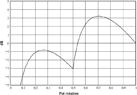
Figure 9.12: The deviation of the unloaded tapped volume control law from an ideal 33 dB log line
A much better approach to a log law is possible if a loading resistor is added to the wiper, as with the loaded linear pot already examined (see Figure 9.10(b) for the circuit arrangement and Figure 9.13 for the control law). If the resistors are correctly chosen, using the ratios given in Figure 9.10(b), the law can be arranged to have no change of slope at the tapping, and the deviation from a 40 dB ideal line will be less than 1 dB over the range from 0 to −38 dB. The exact values of the resistors are given rather than the nearest preferred values. It is clear that this is a very effective way of giving an accurate law over a wide range, and it is widely used in making high-quality slide faders. Note that the accuracy still depends on good control of the track resistance value compared with the fixed resistors.
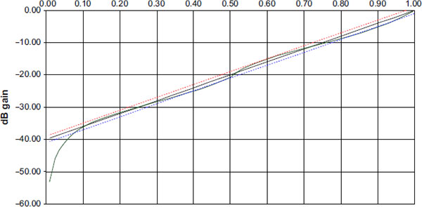
Figure 9.13: The law of a loaded and tapped volume control with −20 dB at the tap. The dotted lines shows the width of a ±1 dB error band around the 40 dB ideal line
If the value of the resistors connected to the tap is such that the loading effect on the previous stage becomes excessive, one possible solution is shown in Figure 9.10(c), where R1 and R2 are kept reasonably high in value, and a unity-gain op-amp buffer now holds the tap point in a vice-like grip due to its low output impedance. The disadvantage is that the noise of the op-amp, and of R1 in parallel with R2, is fed directly through at full level when the wiper is near the tap. Often this will be at a lower level than the noise from the rest of the circuitry, but it is a point to watch. Note that because of the low-impedance drive from the op-amp, the values of the fixed resistors will need to be altered from those of Figure 9.10(b) to get the best control law.
If the best possible noise performance is required, then it is better to increase the drive capability of the previous stage and keep the resistors connected to the tap low in value; if this is done by paralleling op-amps then the noise performance will be improved rather than degraded.
Slide Faders
So far as the design of the adjacent circuitry is concerned, a fader can normally be regarded as simply a slide-operated logarithmic potentiometer. Inexpensive faders are usually made using the same two-slope carbon-film construction as for rotary log volume controls, but the more expensive and sophisticated types use a conductive-plastic track with multiple taps connected to a resistor ladder, as described in the previous section. This allows much better control over the fader law.
High-quality faders typically have a conductive-plastic track, contacted by multiple gold-plated metal fingers to reduce noise during movement. A typical law for a 104 mm travel fader is shown in Figure 9.14. Note that a fader does not attempt to implement a linear-in-dB log scale; the attenuation is spread out over the top part of the travel and much compressed at the bottom. This puts the greatest ease of control in the range of most frequent use; there is very little point in giving a fader precise control over signals at −60 dB.

Figure 9.14: A typical control law for a 104 mm fader, showing how the attenuation is spread out over the upper part of the travel
A so-called infinity-off feature is incorporated into the more sophisticated faders. Figure 9.15(a) shows the straightforward construction used in smaller and less expensive mixers. There is some end resistance Ref at the bottom of the resistive track that compromises the offness, and it is further compromised by the voltage drop down the resistance Rg of the ground wire that connects the fader to the channel PCB.

Figure 9.15: A simple fader (a) and a more sophisticated version (b) with an ‘infinity-off’ section to maximize offness
Figure 9.15(b) shows an infinity-off fader. When the slider is pulled down to the bottom of its travel, it leaves the resistive track and lands on an end section with a separate connection back to the channel module ground. No signal passes down this ground wire and so there is no voltage drop along its length. This arrangement gives extremely good maximum attenuation, orders of magnitude better than the simple fader, though of course ‘infinity’ is always a tricky thing to claim.
Faders are sometimes fitted with fader-start switches; these are microswitches that are actuated when the slider moves from the ‘off’ position.
Active volume controls have many advantages. As explained in the section on preamplifier architectures, the use of an active volume control removes the dilemma concerning how much gain to put in front of the volume control and how much to put after it. An active gain control must fulfill the following requirements:
The gain must be smoothly variable from a maximum, usually well above unity, down to effectively zero, which in the case of a volume control means at least −70 dB. This at once rules out series-feedback amplifier configurations as these cannot give a gain of less than 1. Since the use of shunt feedback implies a phase inversion, this can cause problems with the preservation of absolute polarity.
The control law relating shaft rotation and gain should be a reasonable approximation to a logarithmic law. It does not need to be strictly linear-in-decibels over its whole range; this would give too much space to the high-attenuation end, say around −60 dB, and it is better to spread out the middle range of −20 to −50 dB, where the control will normally be used. These figures are naturally approximate as they depend on the gain of the power amplifier, speaker sensitivity, and so on. A major benefit of active gain controls is that they give much more flexible opportunities for modifying the law of a linear pot than does the simple addition of a loading resistor, which was examined and found somewhat wanting earlier in this chapter.
The opportunity to improve channel balance over the mediocre performance given by the average log pot should be firmly grasped. Most active gain controls use linear pots and arrange the circuitry so that these give a quasi-logarithmic law. This approach can be configured to remove imbalances due to track resistance tolerances.
The noise gain of each amplifier involved should be as low as possible.
As for passive volume controls, the circuit resistance values should be as low as practicable to minimize Johnson noise and capacitative crosstalk.
Figure 9.16 shows a collection of possible active volume configurations, together with their gain equations. Each amplifier block represents an inverting stage with a large gain –A, i.e. enough to give plenty of negative feedback at all gain settings. It can be regarded as an op-amp with its non-inverting input grounded. Figure 9.16(a) simply uses the series resistance of a log pot to set the gain. While you get the noise/headroom benefits of an active volume control, the retention of a log pot with its two slopes and resulting extra tolerances means that the channel balance is no better than that of an ordinary passive volume control using a log pot. It may in fact be worse, for the passive volume control is truly a potentiometer, and if it is lightly loaded differences in track resistance due to process variations should at least partially cancel, and one can at least rely on the gain being exactly 0 dB at full volume. Here, however, the pot is actually acting as a variable resistance, so variations in its track resistance compared with the fixed R1 will cause imbalance; the left and right gain will not even be the same with the control fully up. Given that pot track resistances are usually subject to a ±20% tolerance, it would be possible for the left and right channel gains to be 4 dB different at full volume. This configuration is not recommended.

Figure 9.16: Active volume control configurations
Figure 9.16(b) improves on Figure 9.16(a) by using a linear pot and attempting to make it quasi-logarithmic by putting the pot into both the input and feedback arms around the amplifier. It is assumed that a maximum gain of 20 dB is required; it is unlikely that a preamplifier design will require more than that. The result is the law shown in Figure 9.17, which can be seen to approximate fairly closely to a linear-in-decibels line with a range of 0 to −44 dB. This is a result of the essentially square-law operation of the circuit, in which the numerator of the gain equation increases as the denominator increases. This is in contrast to the loaded linear pot case described earlier, which approximates to a 20 dB line.

Figure 9.17: The control law of the active volume control in (b)
The deviation of the control law from the 44 dB line is plotted in Figure 9.18, where it can be seen that between control rotations of 0.1 and 1, and a gain range of almost 40 dB, the maximum error is ±2.5 dB. This sort of deviation from an ideal law is not very noticeable in practice. A more serious issue is the way the gain heads rapidly south at rotations less than 0.1, with the result that volume drops rapidly towards the bottom of the travel, making it more difficult to set low volumes to be where you want them. Variations in track resistance tend to cancel out for middle volume settings, but at full volume the gain is once more proportional to the track resistance and therefore subject to large tolerances.

Figure 9.18: The deviation of the control law in from an ideal 44 dB logarithmic line
The configuration in Figure 9.16(c) also puts the pot into an input arm and a feedback arm, but in this case in separate amplifiers: the feedback arm of A1 and the input arm of A2. It requires two amplifier stages, but as a result the output signal is in the correct phase. When configured with R = 10 kΩ, R1 = 10 kΩ, R3 = 1 kΩ, and R4 =10 kΩ, it gives exactly the same law as Figure 9.16(b), with the same maximum error of ±2.5 dB. It therefore may be seen as a pointless extra complication, but in fact the extra resistors involved give a greater degree of design freedom.
In some cases a linear-in-decibels line with a range of 44 dB, which is given by the active gain stages already looked at, is considered too rapid; less steep laws can be obtained from a modified version of Figure 9.16(c), by adding another resistor R2 to give the arrangement in Figure 9.16(d). This configuration was used in the famous Cambridge Audio P50 integrated amplifier, introduced in 1970. When R2 is very high, the law approximates to that of Figure 9.16(c). With R2 reduced to 4 kΩ, the law is modified to trace 2 in Figure 9.19; the law is shifted up, but in fact the slope is not much altered, and is not a good approximation to the ideal 30 dB log line, labeled ‘30’. When R2 is reduced to 1 kΩ, the law is as trace 3 in Figure 9.19, and is a reasonable fit to the ideal 20 dB log line, labeled ‘20’. Unfortunately, varying R2 can do nothing to help the way that all the laws fall off a cliff below a control rotation of 0.1, and in addition the problem remains that the gain is determined by the ratio between fixed resistors, for which a tolerance of 1% is normal, and the pot track resistance, with its ±20% tolerance. For this reason none of the active gain controls considered so far is going to help with channel balance problems.

Figure 9.19: The control law of the active volume control in (d)
The Baxandall Active Volume Control
The active volume control configuration in Figure 9.16(e) is due to Peter Baxandall. Like so many of the innovations conceived by that great man, it authoritatively solves the problem it addresses [1]. Figure 9.20 shows the law obtained with a maximum gain of +20 dB; the best-fit ideal log line is now 43 dB. There is still a rapid fall-off at low control settings.

Figure 9.20: The control law of the Baxandall active volume control in (e)
You will note that there are no resistor or track resistance values in the gain equation; the gain is only a function of the pot rotation and the maximum gain set up by R1, R2. As a result quite ordinary dual linear pots can give very good channel matching. When I tried a number of RadioOhm 20-mm-diameter linear pots, the balance was almost always within 0.3 dB over a 46 dB gain range, with occasional excursions to an error of 0.6 dB.
However, the one problem that the Baxandall configuration cannot solve is channel imbalance due to mechanical deviation between the wiper positions. I have only once found that the Baxandall configuration did not greatly improve channel balance; in that case the linear pots I tried, which came from the same Chinese source as the log pots that were provoking customer irritation, had such poor mechanical alignment that the balance improvement obtained was small, and not worth the extra circuitry.
Note that all the active gain configurations require a low-impedance drive if they are to give the designed gain range – don’t try feeding them from, say, the wiper of a balance control pot. The Baxandall configuration inherently gives a phase inversion that can be highly inconvenient if you are concerned with preserving absolute phase, but this can be undone by an inverting tone-control stage.
An important point is that while at first glance the Baxandall configuration looks like a conventional shunt-feedback control, its action is modified by the limited gain set by R1 and R2. This means that the input impedance of the stage falls as the volume setting is increased, but does not drop to zero. With the values shown in Figure 9.21, input impedance falls steadily from a maximum of 10 kΩ at zero gain, to a minimum of 1.27 kΩ at maximum gain. If the preceding stage is based on a 5532 it will have no trouble driving this.

Figure 9.21: A practical Baxandall active volume control, as used in several preamplifier designs
Another consequence of the gain of the A2 stage is that the signals handled by the buffer A1 are never very large. This means that R1, and consequently R2, can be kept low in value to reduce noise without placing an excessive load on the buffer.
All the active volume controls examined here, including the otherwise superior Baxandall configuration, give a gain law that falls rapidly in the bottom tenth of control rotation. It is not easy to see that there is any cure for this.
A Practical Baxandall Active Gain Stage
I have designed several preamplifiers using a Baxandall active volume control [2, 3]. The practical circuitry I employed is shown in Figure 9.21; this includes arrangements to deal with the significant bias currents of the 5532 op-amp [1]. The maximum gain is set to +17 dB by the ratio of R1, R2, to amplify a 150 mV line input to 1 V with a small safety margin.
This active volume-control stage gives the usual advantages of lower noise at gain settings below maximum, and excellent channel balance that depends solely on the mechanical alignment of the dual linear pot – all mismatches of its electrical characteristics are canceled out. Note that in both the preamplifier designs referenced here all the pots were identical at 10 kΩ linear, apart from the question of center detents, which are desirable only on the balance, and treble and bass boost/cut controls.
The values given here are as used in the Precision Preamplifier 96 [3]. Compared with Ref. [2], noise has been reduced slightly by an impedance reduction on the gain-definition network R1, R2. The limit on this is the ability of buffer U1:B to drive R1, which has a virtual earth at its other end. C3 ensures HF stability if there are excess phase-shifts due to stray capacitance. C1 prevents any DC voltages from circuitry upstream from reaching the volume-control stage. The input bias current of U1:B will produce a small voltage drop across R3, and C2 prevents this from reaching the control pot. Since two terminals of the pot are DC blocked, it is now permissible to connect the third terminal to the output of U1:A as no current can flow through the control. The offset voltage at the output of U1:B will be amplified by U1:A, but should still be much too small to have any significant effect on available voltage swing, and it is prevented from leaving this stage by DC-blocking capacitor C4. R4 is a drain resistor to prevent voltage building up on the output due to leakage through C4, and R5 ensures stability by isolating the stage from load capacitance downstream, such as might be caused by the use of screened cable. Note that R4 is connected before R5, to prevent any loss of gain. The amount of loss is of course very small in one stage, but it can build up irritatingly in a large system if this precaution is not observed.
This gain control is used in the second section of the complete preamplifier described in Chapter 11. Table 9.3 gives the noise performance.
Table 9.3 Noise performance of active gain control at various volume settings
Setting |
Noise out (dBu) |
|---|---|
Zero gain |
−114.5 |
Unity gain |
−107.4 |
Full volume |
−90.2 |
The figure at full volume may look a bit mediocre, but results from the use of +17 dB of gain; at normal volume settings the noise output is well below −100 dBu.
Potentiometers and DC
As noted in the previous section, it is never a good idea to have DC flowing through any part of a potentiometer. If there is a DC voltage between the ends of the pot track there will be rustling noises generated as the wiper moves up and down over minor irregularities in track resistance.
Feeding a bias current through a wiper to the next stage tends to create more serious noise because the variations in wiper contact resistance are greater. This tends to get worse as the track surface becomes worn. This practice is often acceptable for FET input op-amps like the TL072, but it is definitely not a good idea for bipolar op-amps such as the 5532 because the bias current is much greater and so therefore is the noise on wiper movement. AC coupling is essential when using bipolar op-amps. If you are using electrolytic capacitors then make sure that the coupling time-constant is long enough for capacitor distortion to be avoided (see Chapter 2).
Motorized Potentiometers
Motorized pots are simply ordinary pots driven by an attached electric motor, heavily geared down and connected to the control shaft through a slipping clutch. This clutch allows manual adjustment of the volume when the motor is off, and prevents the motor stalling when the pot hits the end of its travel; limit switches are not normally used. Motorized pots are now considerably cheaper than they used to be, due to the manufacture of components in China that represent a very sincere homage to designs by ALPS and others, and they appear in lower to middle-range integrated amplifiers. Motorization can be added to any control that uses a rotary pot.
In many ways motorized pots are the ideal way to implement a remote-controlled volume function. There is no variable gain electronics to add noise and distortion, manual control is always available if you can’t find the remote, and their setting is inherently non-volatile, as the knob stays where it was left when you switch off.
A disadvantage is that the ‘feel’ of a motorized pot is pretty certain to be worse than a normal control’s, because of the need for the slipping clutch between the control shaft and the motor; a large-diameter knob helps with this. The channel balance is of course no better than if the same pot was used as a manual control.
Since the motor has to be able to run in either direction, and it is simplest to run it from a single supply, an H-bridge configuration, as shown in Figure 9.22, is used to drive it. Normally all four transistors are off. To run the motor in one direction Q1 and Q4 are turned on; to run in the other direction Q2 and Q3 are turned on. The H-bridge and associated logic to interface with a microcontroller can be obtained in convenient ICs such as the BA6218 by Rohm. This IC can supply an output current of up to 700 mA. Two logic inputs allow four output modes: forward, reverse, idle (all H-bridge transistors off), and dynamic braking (motor shorted via ground). The logic section prevents input combinations that would turn on all four devices in the H-bridge and create (briefly) electronic mayhem.

Figure 9.22: Control circuitry for a motorized volume control
It would appear that there might be problems with electrical noise from the motor getting into the audio circuitry, but I have not myself found this to be a problem. In the usual version the motor is screened with a layer of what appears to be grain-oriented silicon steel (GOSS) to keep magnetic effects under control, and the motor terminals are a long way from the audio terminals. A 100 nF capacitor across the motor terminals, and as close to them as practicable, is always a good idea. The motor should be driven from a separate non-audio supply unless you’re really looking for trouble; motorized controls with 5 V motors are popular as they can run off the same +5 V rail as a housekeeping microcontroller. Once again I have never had problems with motor noise interfering with a microcontroller.
Linear faders, as used on mixing consoles, are also sometimes motorized, not for remote control, but to allow previously stored fader movements to be played back in an automatic mixdown system. A linear servo track next to the audio track allows accurate positioning of the fader. Motorization has usually been done by adding a small electric motor to one end of the fader, and moving the control knob through a mechanism of string and pulleys that is strongly reminiscent of an old radio dial. Such arrangements have not always been as reliable as one might have hoped.
Stepped Volume Controls
The great feature of potentiometer-based volume controls is that they have effectively infinite resolution, and you can set exactly the level you require. If, however, you are prepared to forgo this and accept a volume control that changes in steps, a good number of new possibilities open up, and in return promise much greater law accuracy and channel balance. The technologies available include rotary-switched resistive attenuators, relay-switched resistive attenuators, switched multi-tap transformers, and specialized volume-control ICs. These options are examined below.
The obvious question is: how small a step is needed to give satisfactory control? If the steps are made small enough they are imperceptible, provided there are no switching transients, but there are powerful economic reasons for not using more steps than necessary. Two-decibel steps are widely considered acceptable for in-car entertainment (implemented by an IC) but my view is that serious hi-fi requires 1-dB steps.
Switched Attenuator Volume Controls
For high-end products where the imperfections of a ganged-potentiometer volume control are not acceptable, much superior accuracy can be achieved by using switched attenuators to control level. It is well known that the BBC for many years used rotary faders that were stud-switched attenuators working in 2-dB steps; some of these were still in use in 1961.
The normal practice is to have a large rotary switch that selects a tap on a resistor ladder; since the ladder can be made of 1% tolerance components the channel matching is much better than that of the common dual-gang pot. A stereo control naturally requires two resistor ladders and a two-pole switch. The snag is of course the much greater cost; this depends to a large extent on how many control steps are used. The resistor ladders are not too costly, unless exotic super-precision parts are used, but two-pole switches with many ways are neither cheap nor easy to obtain.
At the time of writing, one commercial preamp offers 12 5-dB steps; the component cost has been kept down by using separate switches for left and right channels, which is not exactly a triumph of ergonomics. Another commercial product has an 11-position ganged switched attenuator. In my opinion neither offers anything like enough steps.
The largest switches readily available are made up from one-pole 12-way wafers. The most common version has a break-before-make action, but this causes clicky transients due to the interruption of the audio waveform. Make-before-break versions can usually be obtained and these are much more satisfactory as the level changes as the switch is rotated are much smaller, and the transients correspondingly less obtrusive.
Moving beyond 12-way, a relatively popular component for this sort of thing is a 24-position switch from the ELMA 04 range; this seems to be the largest number of ways they produce. A bit of care is needed in selecting the part required as one version has 10 μm of silver on the contracts with a protective layer of only 0.2-μm-thick gold. This very thin layer is for protection during storage and transport only and in use will wear off quite quickly exposing the silver, which is then subject to tarnishing, with the production of non-conductive silver sulfide; this version should be avoided unless used in a sealed environment. Other versions of these switches have 3-μm-thick gold on the contacts, which is much more satisfactory. They can be obtained with one, two, or four 24-way wafers, but they are not cheap. At the time of writing (January 2009) two-wafer versions are being advertised by third parties at about $130 each, which means that in almost all cases the volume switch is going to cost a lot more than the rest of the preamplifier parts put together.
A switched attenuator can be made very low impedance to minimize its own Johnson noise and the effect of the current noise of the following stage. The limiting factors are that the attenuator input must present a load that can be driven with low distortion from the preceding stage, and that the resistor values at the bottom of the ladder do not become too small for convenience. An impedance of around 1000 Ω from top to bottom is a reasonable choice. This means that the highest output impedance (which is at the −6 dB setting, a very high setting for a volume control) will be only 250 Ω. This has a Johnson noise of only −128.2 dBu (22 kHz bandwidth, 25ºC) and is unlikely to contribute much to the noise output of a system. The choice of around 1000 Ω does assume that your chosen range of resistors goes down to 1 Ω rather than stopping at 10 Ω, though if necessary the lower values can of course be obtained by paralleling resistors.
Assuming you want to use a 12-way switch, a possible approach is to use 12 steps of 4 dB each, covering the range 0 to −44 dB. My view is that such steps are too large, and 2 dB is much more usable, but you may not want to spend a fortune on a rotary switch with more ways. In fact, 1-dB steps are really required so you can always get exactly the volume you want, but implementing this with a single rotary switch is going to be very difficult, as it implies something like a 60- or 70-way switch. My own preamplifier just happens to be a relay-switched Cambridge Audio 840E with some 90-odd 1-dB steps.
There is no reason why the steps have to be equal in size, and it could be argued that the steps should be smaller around the center of the range and larger at the top and bottom, to give more resolution where the volume control is most likely to be used. It does not really matter if the steps are not exactly equal – the vital thing is that they should be identical for the left and right channels to avoid image shift.
Figure 9.23(a) shows a typical switched attenuator of this sort, with theoretically exact resistor values, so the size of each step is 4.0000 dB; in fact each step is accurate to five decimal places. In view of resistor tolerances, such accuracy may appear pretty pointless, apart from the warm feeling it produces, but it costs nothing to start off with more accuracy than you need. The total resistance of the ladder is 1057 Ω, which is a very reasonable load on a preceding stage, so long as it is implemented with 5532s or similar.

Figure 9.23: A 12-way switched attenuator volume control. (a) gives the theoretical resistor values, (b) is the best accuracy with E24 resistor values, and (c) shows how the step errors are much reduced by using E96 values
A lot depends on what range of resistor values you have access to. When I began to design preamplifiers, E12 resistors (12 values per decade) were the norm, and E24 resistors (24 values per decade) were rather rare and expensive. This is no longer the case, and E24 is freely available. Figure 9.23(b) shows the same attenuator with the nearest E24 value used for each resistor. The attenuation at each tap is still very accurate, the error never exceeding 0.12 dB except for the last tap, which is 0.25 dB high; this could be cured by making R12 a parallel combination of 6.8 and 330 Ω and making R11 3.9 Ω, which reduces the last-tap error to 0.08 dB.
The next most prolific resistor range is E96, with no less than 96 values in a decade – nobody seems interested in making an E48 range as such, though it is of course just a subset of E96. Using the nearest E96 value in the attenuator, we get Figure 9.23(c), where the taps are accurate to within 0.04 dB; remember that this assumes that each resistor is exactly the value it should be and does not incorporate any tolerances. The improvement in accuracy is not enormous, and if you can get a tighter tolerance in the E24 range than E96, E24 is the preferred option.
There is also an E192 resistor range, but it is rather rare, and there seems to be no pressing need to use so many different values in volume-control attenuators.
Almost all the work in the design of a switched attenuator is the calculation of the resistor values in the ladder. A spreadsheet model is the best way to do this. Putting in likely component values and attempting to tweak them by hand is a most unpromising approach, because all the values interact and you will boil off your sanity. A systematic approach using a spreadsheet is the best way. This is probably the simplest:
Decide the approximate total resistance of the resistor ladder.
Decide the step size, say 4 dB.
Take a two-resistor potential divider, where the sum of the resistors equals the desired total resistance, and choose exact values for a 4 dB attenuation; work back by trial and error to get an exact E24 value for the top resistor. (An exact E24 value at the top of the ladder is not essential, but it is convenient.)
Now split the bottom resistor into two, so that another 4 dB attenuator results. Check that the attenuation really is correct, because an error will propagate through the rest of the process, and you will have to go back and do it again from that point. Repeat this step until you have enough resistors in the ladder for the number of taps required.
When the table of resistor values is complete, for each resistor pick the nearest value from the E-series you are using.
You will then have constructed something like the spreadsheet shown in Table 9.4, which gives the E24 resistor values shown in Figure 9.23(b). The chosen value at the top of the ladder is 390 Ω. The spreadsheet has been set up to give more information than just the resistor value and the tap attenuation; it gives the voltage at each tap for a given input (10 Vin this case) in column 5, the output impedance of each tap in column 6, the step size in dB in column 8, and the absolute error for each tap in column 9. It also gives the total resistance of the ladder, the current through it for the specified input voltage, and the resulting power dissipation in each resistor in column 7. The last parameter is unlikely to be a major concern in an audio attenuator, but if you’re working with very low impedances to minimize noise, it is worth keeping an eye on.
Table 9.4 A spreadsheet that gives all the relevant information about a divider ladder for a switched attenuator

Before the design work begins you must consider the stages before and after the attenuator. It is highly recommended that the attenuator input is driven from a very low impedance such as the output of an op-amp with plenty of negative feedback, so the source impedance can be effectively considered as zero and does not enter into the calculations. The loading on the output of the attenuator is more of a problem. You can either take loading on the output into account in the calculations, in which case the shunting effect of the load must be incorporated into step 3 above, or else make the input impedance of the next stage so high that it has a negligible effect.
As an example, the E24 network in Figure 9.23(b) was calculated with no allowance for loading on the output. Its highest output impedance is 253 Ω at tap 3, so this is the worst case for both loading sensitivity and noise. If a load of 100 kΩ is added, the level at this tap is only pulled down by 0.022 dB. A 100 kΩ input impedance for a following stage is easy to arrange, so the extra computation required in allowing for loading is probably not worthwhile unless for some very good reason the loading is much heavier. The Johnson noise of 253 Ω is still only −128.2 dBu. If you feel you can afford 24-way switches, then there is rather more flexibility in design. You could cover from 0 to −46 dB in 2-dB steps, 0 to −57.5 dB in 2.5-dB steps, or 0 to −69 dB in 3-dB steps. There are almost infinite possibilities for adopting varying step sizes.
Table 9.5 shows the resistor values for 0 to −46 dB in 2-dB steps, Table 9.6 gives those for 0 to −57.5 dB in 2.5-dB steps, and Table 9.7 gives the values for 0 to −69 dB in 3-dB steps. All three tables give the nearest E24 and E96 values, and the resulting errors. Note the first two versions start off with a 220 Ω resistor at the top, but on moving from 2- to 2.5-dB steps, the resistors toward the bottom naturally get smaller to give the greater attenuation required, and the total ladder resistance falls from 1060 to 866 Ω. To prevent the resistor values becoming inconveniently small, the 3-dB step version starts off with a higher value resistor of 430 Ω at the top; this increases the total resistance of the ladder to 1470 Ω and raises the maximum output impedance to 368 Ω at tap 3. The Johnson noise of 368 Ω is naturally higher at −126.5 dBu, but this is still very low compared with the likely noise from amplifier stages downstream.
Table 9.5 Resistor values and accuracy for a 2-dB step switched attenuator
Table 9.6 Resistor values and accuracy for a 2.5-dB step switched attenuator

Table 9.7 Resistor values and accuracy for a 3-dB step switched attenuator

The exact values on the left-hand side of each table can be scaled to give the total divider resistance required, but it will then be necessary to select the nearest E24 or E96 value manually. If you are increasing all the resistances by a factor of 10, then the same E24 or E96 values with a zero added can be used. The average of the absolute error for all 24 steps is shown at the bottom of each section; note that simply taking the average error would give a misleadingly optimistic result because the errors are of random sign and would partially cancel.
If 24 volume steps are not enough for you, then a different approach is required. Using relays, a microcontroller and an inexpensive shaft encoder, it is relatively simple to come up with a system that emulates a rotary switch with as many ways as desired, but you will need an awful lot of relays. Another approach is to use relays in a ladder attenuator, which greatly reduces the relay count. This is dealt with in the next section. As soon as a microcontroller is introduced, then there is of course the possibility of infrared remote control.
Another solution is to use two rotary switches: one for coarse volume control and the other for vernier volume control, the latter perhaps in 1-dB steps. While this is a workable approach, it is not exactly user-friendly. A buffer stage is usually desirable to prevent the second attenuator from loading the first one; the second attenuator should present a constant load, but it is a heavy one. The total loading of the two attenuators could also present an excessive load to the stage before the first attenuator.
A rotary switch does not of course have the smooth feel of a good potentiometer. To mitigate this, a switched volume control may need a large-diameter weighted knob, possibly with some sort of silicone damping. Sharp detents and a small knob do not a good volume control make.
Relay-Switched Volume Controls
The ultimate development in stepped volume controls is the relay ladder attenuator. This allows any number of steps to be employed.
The design of a good relay volume control is not as simple as it may appear. If you try to use a binary system, perhaps based on an R−2R network, you will quickly find that horrible transients erupt on moving from, say, 011111 to 100000. This is because relays have an operating time that is both long by perceptual standards, and somewhat unpredictable. It is necessary to use logarithmic resistor networks with some quite subtle relay timing.
Currently the highest expression of this technology is the Cambridge Audio 840A Integrated amplifier and 840E preamplifier. The latter uses second-generation relay volume control technology. A rather unexpected feature of relay volume controls is that having purchased a very sophisticated preamplifier, where the precision relay control is the major unique feature, some customers then object to the sound of the relays clicking inside the box when they adjust the volume setting. You just can’t please some people.
Transformer-Tap Volume Controls
There are other ways of controlling volume than with resistors. At the time of writing (2009) there is at least one passive preamplifier on the market that controls volume by changing the taps on the secondary of a transformer. This should at least give a low output impedance, but there are several potential problems with this idiosyncratic approach – transformers are well known to fall much further short of being an ideal component than most electronic parts do. They can introduce frequency response irregularities, LF distortion, and hum. They are relatively heavy and expensive, and the need for a large number of taps on the secondary puts the price up further. A multi-way switch to select the desired tap must also be paid for.
The unit I have in mind has only 12 steps, apparently each of 4 dB. These are very coarse steps for a volume control – unacceptably so, I would have thought. Twenty-four-way switches are available (see the section on switched attenuator volume controls above) but they are expensive, and there might be some interesting challenges in fitting 24 taps into a transformer design.
Integrated Circuit Volume Controls
Specialized volume-control ICs based on switched networks have been around for a long time, but have only recently reached a level of development where they can be used in high-quality audio. Early versions had problems with excessively large volume steps, poor distortion performance, and nasty glitching on step changing. The best contemporary ICs are greatly improved; a modern example is the PGA2310 from Burr-Brown (Texas Instruments), which offers two independent channels with a gain range from +31.5 to −95.5 dB in 0.5-dB steps, and is spec’d at 0.0004% THD at 1 kHz for a 3 Vrms input level. The IC includes a zero crossing detection function intended to give noise-free level transitions. The concept is to change gain settings on a zero crossing of the input signal, and so minimize audible glitches. Gain control is by means of a three-wire serial interface, which is normally driven by a rotary encoder and a microcontroller such as one of the PIC series.
The Yamaha YAC523 has a similar specification but incorporates seven gain-controlled channels for AV applications.
Balance Controls: Passive
The balance control on a preamplifier adjusts the relative gain of the left and right channels, in order to move the stereo stage to the left or right. As you would expect, increasing the left gain moves things to the left. A balance control does not have to make radical changes to signal level to do its job. Introducing a channel gain imbalance of 10 dB is quite enough to shift the sound image completely to one side, so it appears to be coming from one loudspeaker only, and there is nothing to be gained by having the ability to fade out one channel completely. A central detent on the control is highly desirable.
The ideal hi-fi balance control is not a mixer panpot (see Chapter 17 on mixer subsystems). Since the balance control is usually a set-and-forget function that does not require readjustment unless the listening room is rearranged, there is no requirement that the overall volume remains exactly constant when the balance is adjusted. The ideal hi-fi balance control will have no attenuation when set centrally, and when moved to left or right will attenuate only one channel without affecting the gain of the other; to implement this passively in a pot requires a special design, but this is not a problem as they are available from several manufacturers. If there is attenuation at the central position then it needs to be made up by extra amplification either before or after the balance control, and this means that either the overload margin or the noise performance will be compromised to some degree.
Figure 9.24 shows the various forms of passive balance control; only the right channel is shown in the first three cases. Anticlockwise movement of the control is required to introduce attenuation into the right channel and shift the sound image to the left. In Figure 9.24(a) a simple pot is used. If this has a linear track it will give a 6 dB loss when set centrally – this means that an extra 6 dB of gain has to be built into the system, and the noise/headroom compromise is too great. If a log law is used for one channel, and an anti-log law for the other, the central loss can be made smaller, say 3 dB or less.

Figure 9.24: Passive balance controls
However, the uncertainties of log-law tolerancing means it will not be possible to guarantee that the channel gains are identical when the control is centralized. The ultimate expression of this is the special balance pot shown in Figure 9.24(b), where the top half of the track is made of a low-resistance material, so that neither channel is attenuated at the central position. On moving the control clockwise the right channel wiper stays on the low-resistance section and gain stays at 0 dB, while the left wiper moves on to the normal log/anti-log section and the signal is attenuated. Another balance control option is shown in Figure 9.24(c), where a linear pot is used with a pull-up resistor so the attenuation at the central position is less than 6 dB. With the values shown the loss for each channel with the control central is −2.6 dB. More information on what is essentially a panpot configuration (though not in this case a panpot law) can be found in Chapter 17.
The economical method of Figure 9.24(d) was once popular as only a single pot section is required. Unfortunately it has the snag that the relatively high resistance between wiper and track causes serious degradation of the interchannel crosstalk performance. If the resistance values are reduced to lower Johnson noise, the track-wiper resistance is unlikely to decrease proportionally and the crosstalk will be worsened. With the values shown the loss for each channel with the control central is −3.2 dB. This loss can be reduced by decreasing the value of R1, R2 with respect to the pot, but this puts a correspondingly heavier load on the preceding stages when the control is well away from central.
Some preamplifier designs have attempted to evade the whole balance control problem by having separate but concentric volume knobs for left and right channels. The difficulty here is that almost all the time the volume only will require adjustment, and the balance function will be rarely used; it is therefore highly desirable that the left and right knobs are linked together in some sort of high-friction way so that the two normally move together. This introduces some awkward mechanical complications.
Active Balance Controls
An active balance control is configured so that it makes a small adjustment to the gain of each channel rather than introducing attenuation, so the noise/headroom compromise can be avoided altogether. Since all active preamplifiers have at least one gain stage, the extra complication is likely to be minimal. It is not desirable to add an extra active stage just to implement the balance function.
Figure 9.25(a) shows an active balance control that requires only a single-gang pot. However, it suffers from the same serious disadvantage as the passive version in Figure 9.24(d): the wiper connection acts as a common impedance in the two channels and causes crosstalk. This kind of balance control cannot completely fade out one channel as it is not possible to reduce the stage gain below unity, and in fact even unity cannot be achieved with this configuration. With the values shown the gain for each channel with the control central is +6.0 dB. With the control fully clockwise the gain increases to +9.4 dB, and decreases to +4.4 dB with it fully anticlockwise; the range is deliberately quite restricted. It is a characteristic of this arrangement that the gain increase on one channel is greater than the decrease on the other.
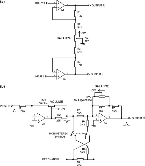
Figure 9.25: Active balance controls
Figure 9.25(b) shows an active balance control combined with an active gain control and mono/stereo switching. This is the configuration shown above in Figure 9.16(d), and was used in the original Cambridge Audio P-series amplifiers; there A1 was a simple two-transistor inverting stage and A2 an even simpler single transistor. The left-hand section of volume control RV1 is the feedback resistance for A1, while the right-hand section forms part of the input resistance to shunt stage A2, both changing to give a quasi-logarithmic law when the control is altered. The balance control RV2 is a variable resistance in the shunt-feedback network of A2. The mono/stereo switch feeds the virtual-earth node of A2 with both channels via R3, R4 when in mono mode. The circuit handily avoids phase inversion of the output.
Mono/Stereo Switches
It was once commonplace for preamplifiers to have mono/stereo switches, which allowed a mono source to be played over both channels of a stereo amplifier system. Some of these were configured so that the two channels were simply joined together somewhere in the middle of the preamp stages, which was not very satisfactory unless the unused input was terminated in a low impedance to minimize noise. More sophisticated versions allowed either the left or the right input to be routed to both outputs.
Since all modern sources are at least stereo, mono/stereo switches are now rarely if ever fitted.
Width Controls
Another facility that has become rare is the width control. Summing a small proportion of each channel into the other reduces the width of the sound image, and this was sometimes advocated as a small width reduction would make the image less associated with the loudspeakers, and so give a stronger illusion of acoustic reality. This of course runs directly counter to more contemporary views that very high levels of interchannel isolation are required to give a good stereo image. This is flat-out untrue; it was established long ago by the BBC, in extensive testing before the introduction of stereo broadcasting, that a stereo separation of 20–25 dB is enough to give the impression of full image width.
By cross-feeding anti-phase signals, the width of a stereo image can be increased. A famous circuit published by Mullard back in 1972 [4] gave continuous variation between mono, normal, and enhanced-width stereo. It was stated that anti-phase cross-feed of greater than 24% should not be used as it would cause the sound image to come apart into two halves.
[1] P. Baxandall, Audio gain controls, Wireless World (November 1980) pp. 79–81.
[2] D. Self, A precision preamplifier, Electronics World (October 1983).
[3] D. Self, Precision Preamplifier 96, Electronics World (July/August and September 1996).
[4] M.J. Rose (Ed.), Transistor Audio and Radio Circuits, second ed., Mullard, 1972, p. 180.
Small Signal Audio Design; ISBN: 9780240521770
Copyright © 2010 Elsevier Ltd; All rights of reproduction, in any form, reserved.