
5
Design and Analysis of a Wireless Monitoring Network for Transmission Lines in the Smart Grid
In this chapter, we design a monitoring network for the transmission lines in the smart grid, taking advantage of the existing utility backbone network. We propose several centralized power allocation schemes to set the benchmark for deployment and operation of the wireless sensor nodes in the monitoring system. A distributed power allocation scheme is proposed to further improve the power efficiency of each sensor node for realistic cases with dynamic traffic. Numerical results and a case study are provided to demonstrate the proposed schemes.
5.1 Background and Related Work
5.1.1 Background and Motivation
The power transmission line is an important part of the power grid. It is critical for the control center to monitor the status of the transmission line (e.g. the working status of the key components, the voltage and phase of the power, etc.), and its surrounding environment (e.g. the temperature, the humidity, etc) so that necessary actions can be taken in time to prevent disastrous outcomes. However, monitoring the transmission line is not an easy task for a traditional power grid, because of its vast expanse as well as because parts of it are deployed in remote areas, such as deserts and mountains.
The smart grid, which integrates an advanced communication system to the traditional power grid [4, 6–8, 10, 34, 82–84], makes it possible to install and upgrade the monitoring equipment along transmission lines to obtain precise and timely status information. In the construction of power transmission lines, an optical ground wire (OPGW) [85] is usually installed alongside them [86]. Therefore, the monitoring data can be transmitted to the control center almost immediately once the data gets access to OPGW. However, it is not economical to deploy an OPGW gateway at each transmission tower. In practice, the gateways are deployed far away from each other (e.g. every 20 kilometers) [87].
In this chapter, we design a monitoring network for the transmissionline, based on the existing OPGW. The designed monitoring network consists of hundreds of wireless sensor nodes that are deployed on top of selected power line transmission towers. Each wireless sensor is a piece of comprehensive hardware which includes several physical sensors and a wireless transmission module. The physical sensors (e.g. current transformers [88, 89]) are deployed to measure the electric current status (e.g. electric flow, phase status, etc.) and line positions (e.g. sag) [90–92]. The wireless transmission module delivers the monitored data to the control center for further analysis. Wireless technology has been widely adopted in the smart grid. For example, the smart grid in China has been allocated a dedicated spectrum for wireless transmission [93, 94].
Although the transmission line carries electricity, it is too powerful to directly support a wireless sensor node. Therefore, we assume that the wireless sensors are powered by batteries coupled with green energy generation (e.g. solar power or wind turbines). Green energy and energy harvesting techniques have been studied to show their availability to support general wireless sensor networks as well as communication networks in the smart grid [10, 95, 96]. With green energy, the wireless monitoring network can be deployed in a more flexible way. Now that the sensors are powered by green energy, we need to design a proper power supply component (the size of solar panel and the capacity of the battery) for each sensor node so that the deployment and maintenance costs can be budgeted without much waste. Note that the physical sensors are assumed to be powered at a constant rate thus our focus is on the wireless transmission module.
The most imperative requirement of the transmission line monitoring network is timely delivery of data while being energy efficient. To tackle this issue, we propose several centralized schemes to estimate the power consumption of each sensor. Specifically, the first scheme is designed to minimize the total power consumption of all sensors. Due to its complexity, we relax the approach to minimizing the total transmission efficiency while meeting the latency requirement. We also introduce a game theoretical scheme for faster computation and two more schemes with partial fixed variables for practical application to a large network. The results of the centralized schemes are used as benchmarks for network deployment and operational settings. In practical field operations, the gathered/generated monitoring data is not always at its maximum for each sensor, and the frequency of gathering such data is lower than that of the worst‐case scenario considered in the centralized schemes. Moreover, centralized schemes are not applicable in practical operations due to the real‐time transmission of the monitoring network. Therefore, we propose an adaptive distributed power allocation scheme so that real‐time transmission can be achieved while each sensor can be more energy efficient by taking into consideration the dynamic transmitting data. The proposed distributed scheme is guaranteed to be more power efficient since it is bounded by the benchmark settings from the centralized schemes.
5.1.2 Related Work
The cyber‐physical system of the smart grid, which has been studied by many researchers [34, 6, 8, 10, 97] includes data transmission, power management, cybersecurity, etc. Only a few researchers works mention the monitoring network of the power line transmission system. In most cases, the monitoring systems for high‐voltage power transmission lines takes into consideration both electric current and the positions of the transmission lines so that overload, phase unbalance, fluctuation, etc. can be avoided or reduced, and some situations such as sagging and galloping can be tracked by the control center.
Current transformers (CTs) are typically used for current measurement [88, 89]. Some existing devices can directly or indirectly measure the sag of transmission lines. For example, Ren et al. proposed a dynamic line rating system to monitor the line sag under complex climates (e.g. heavy rains, heavy snow, strong wind, etc.) [90]. Huang et al. proposed an on‐line scheme to monitor the icing density and type of the transmission line [92]. Sun et al. proposed a high‐voltage transmission‐line monitoring system based on magnetoresistive sensors [91] that calculate both the current flow and the line positions from the magnetic field of the phase conductors. Although those monitoring systems work properly for a section of transmission lines, they lack a data transmission technology to deliver the measured data to the control center over long distances in a short period of time. Therefore, the control systems of the smart grid, such as updated supervisory control and data acquisition (SCADA) and general network operations center (NOC), are not fully utilized to provide real‐time monitoring and reaction.
Instead of monitoring technologies for a specific component or a section between two towers, our focus is on the long‐distance data delivery of the monitoring network's information to the control center so that the advance control system in the smart grid can take action quickly when necessary. Lin et al. proposed a power transmission line monitoring frame based on a wireless sensor netword [97]. A traditional wireless mesh sensor network was studied due to multiple sensors on each tower. Routing protocols and hybrid medium access control (MAC) were also proposed to increase the energy efficiency of the sensor network. However, a renewable energy source was not considered, and the transmission data rate was not guaranteed by the proposed schemes. Energy efficiency in wireless sensor networks and multiaccess networks has also been widely studied [74–76]. However, traditional approaches generally assume that the data is delay tolerant and the nodes are subject to unrecoverable failures (e.g. a fully discharged battery). Therefore, we cannot apply the power allocation schemes directly from those works. In our work, we propose a utility function that not only targets the energy efficiency of the wireless transmission module but is also adaptive to different link delay and data traffic requirements.
The rest of this chapter is organized as follows. In Section 5.2, we present the transmission line monitoring network model in the future smart grid. In Section 5.3, we propose several centralized power allocation schemes in which the results can be used as a benchmark for the sensor network design. We also propose a distributed scheme based on the benchmark to deal with dynamic traffic loads for practical cases. In Section 5.6, we show the analysis and numerical results for the centralized schemes. We also conduct a case study to demonstrate the performance of the distributed scheme. We conclude the work in Section 5.7.
5.2 Network Model
In the smart grid, an OPGW network is deployed in parallel with a power transmission line and connected to the control center [85, 86]. A gateway to the OPGW network is deployed every few miles so that uploading and downloading of data to and from the data center can be achieved even if the power line towers are in remote areas. The proposed transmission line monitoring network consists of hundreds of wireless sensor nodes (we will use both sensor and transmitter interchangeably for simplicity hereafter) that are deployed on top of selected towers. The wireless sensors are powered by green energy (e.g. solar power or wind turbine); thus a wireless monitoring network can be deployed in a more flexible way. The combination of wireless technology and green energy also makes it more convenient to maintain or upgrade the sensors if it becomes necessary in the future. In the monitoring system, each sensor gathers the operating status of the transmission line and monitors its surrounding environment. Each sensor also delivers its monitoring data to the control center through the nearest OPGW gateway (gateway hereafter). Due to the long distance between two neighboring gateways, the monitoring network in between forms a multihop wireless network with a physical chain topology. An OPGW gateway usually has its own power supply from a reliable power source, and it is physically attached to the OPGW. In this chapter, our focus is on the multihop wireless part of the monitoring network between two neighboring gateways.
Figure 5.1 shows the studied section of the wireless monitoring network. As shown in the figure, ![]() and
and ![]() are two neighboring OPGW gateways. The transmission between
are two neighboring OPGW gateways. The transmission between ![]() and
and ![]() is achieved by two multihop wireless networks consisting of sensors. It is not necessary to mount sensors on all the towers; for simplicity, we show only the towers with sensors in Figure 5.1. Let
is achieved by two multihop wireless networks consisting of sensors. It is not necessary to mount sensors on all the towers; for simplicity, we show only the towers with sensors in Figure 5.1. Let ![]() be the set of total sensors between
be the set of total sensors between ![]() and
and ![]() , where
, where ![]() includes
includes ![]() sensors that that form a network uploading data to gateway
sensors that that form a network uploading data to gateway ![]() , and
, and ![]() includes another
includes another ![]() sensors that form a network uploading data to gateway
sensors that form a network uploading data to gateway ![]() . Without loss of generality, we focus on the sensors in
. Without loss of generality, we focus on the sensors in ![]() in the rest of the discussion. Note that the distance between two towers should be based on practical deployment. As mentioned before, the sensors upload their monitoring data in a multihop way; that is, sensor
in the rest of the discussion. Note that the distance between two towers should be based on practical deployment. As mentioned before, the sensors upload their monitoring data in a multihop way; that is, sensor ![]() uploads its data to its neighbor
uploads its data to its neighbor ![]() , and
, and ![]() aggregates its own data to the data received from
aggregates its own data to the data received from ![]() and then sends the aggregated data to
and then sends the aggregated data to ![]() . All the data from
. All the data from ![]() will be uploaded to
will be uploaded to ![]() and then be transmitted to the control center through OPGW. Since the transmission over OPGW is much faster than the wireless proportion and is properly powered and well maintained, we thus focus on the power allocation over the sensors of the wireless multihop network. For simplicity, we assume that the networks work over half duplex transmission. Moreover, the focus of the monitoring network is on its uplink transmission, during which the sensors deliver data to the gateway.
and then be transmitted to the control center through OPGW. Since the transmission over OPGW is much faster than the wireless proportion and is properly powered and well maintained, we thus focus on the power allocation over the sensors of the wireless multihop network. For simplicity, we assume that the networks work over half duplex transmission. Moreover, the focus of the monitoring network is on its uplink transmission, during which the sensors deliver data to the gateway.
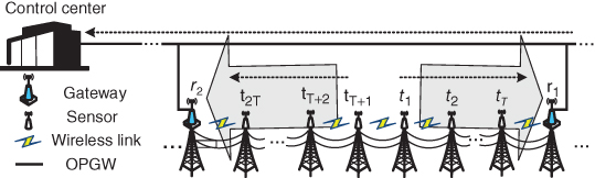
Figure 5.1 A section between two towers with fiber‐optic connections.
For the transmission link ![]() , it is similar to the multiaccess wireless system at receiver
, it is similar to the multiaccess wireless system at receiver ![]() . The sensors in the monitoring network keep sending data; therefore
. The sensors in the monitoring network keep sending data; therefore ![]() not only receives the signal from
not only receives the signal from ![]() but also the interference from other sensors, as shown in Figure 5.2. In general,
but also the interference from other sensors, as shown in Figure 5.2. In general, ![]() receives interference not only from
receives interference not only from ![]() but also from other sensors, such as those in
but also from other sensors, such as those in ![]() and beyond. Since the sensors are placed apart from each other, interference from those sensors several hops away is low in practice. For better illustration, we only consider the interference from the sensors in
and beyond. Since the sensors are placed apart from each other, interference from those sensors several hops away is low in practice. For better illustration, we only consider the interference from the sensors in ![]() in this chapter.
in this chapter.
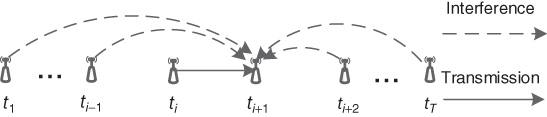
Figure 5.2 Source of interference for link 
5.3 Problem Formulation
To make the illustration clearer, we list the key variables and notations in Table 5.1 that are used throughout the rest of the chapter.
Table 5.1 Key sets and variables.
| Sets | |
| set of sensors/transmitters | |
| set of transmitting power of all | |
| set of path gains | |
| Variables | |
| gathered and generated data at | |
| outgoing data from | |
| transmitting power of | |
| output SINR measured at | |
| path gain of |
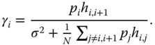
In wireless transmissions, additional energy consumption changes the fundamental tradeoff between energy efficiency and data rate [81]. The effective data rate takes into account the transmission error, data retransmission, packet loss, etc. Generally, with a given situation, a transmitter is required to transmit at a higher power in order to achieve a higher signal‐to‐interference‐plus‐noise ratio (SINR). And a higher SINR leads to a higher transmission rate, since the probability of successful transmission increases with respect to SINR. For a transmitting sensor ![]() , its effective transmission rate at the receiving sensor
, its effective transmission rate at the receiving sensor ![]() is widely adopted as [74–76]
is widely adopted as [74–76]
where ![]() is the theoretical transmission rate, and
is the theoretical transmission rate, and ![]() is the SINR of
is the SINR of ![]() at
at ![]() , which is computed as
, which is computed as
In Eq. (5.1), ![]() is the efficiency function (or normalized transmission data rate), which is assumed to be increasing, continuous, and S‐shaped (sigmoidal; more specifically, there is a point above which the function is concave and below which the function is convex [76]) with
is the efficiency function (or normalized transmission data rate), which is assumed to be increasing, continuous, and S‐shaped (sigmoidal; more specifically, there is a point above which the function is concave and below which the function is convex [76]) with ![]() and
and ![]() . This efficiency function is commonly adopted as [74–76]
. This efficiency function is commonly adopted as [74–76]
where ![]() is the packet length. Without loss of generality, we take FSK as an example for discussion. Then we have
is the packet length. Without loss of generality, we take FSK as an example for discussion. Then we have
Figure 5.3 shows the S‐shaped curve of the efficiency function Eq. (5.3). In Eq. (5.2), ![]() is the transmission power of
is the transmission power of ![]() , where
, where
and ![]() is the maximum transmission power.
is the maximum transmission power. ![]() in Eq. (5.2) is the variance of the zero‐mean white Gaussian noise,
in Eq. (5.2) is the variance of the zero‐mean white Gaussian noise, ![]() is the path gain of
is the path gain of ![]() at
at ![]() , and
, and ![]() is the processing gain. Note that
is the processing gain. Note that ![]() does not cause interference to
does not cause interference to ![]() due to the assumption of half‐duplex transmission. Moreover, it is practical to assume that the transmitter and receiver pair have a line‐of‐sight (LOS) link. Then the path gain of a transmission link is mainly based on carrier frequency and physical distance between the transmitter and the receiver. Therefore, for simplicity, we adopt the free space path loss model to calculate
due to the assumption of half‐duplex transmission. Moreover, it is practical to assume that the transmitter and receiver pair have a line‐of‐sight (LOS) link. Then the path gain of a transmission link is mainly based on carrier frequency and physical distance between the transmitter and the receiver. Therefore, for simplicity, we adopt the free space path loss model to calculate ![]() as
as
where ![]() in kilometers is the distance between two transmitters. Note that the distance between two transmitters may not be the distance between two consecutive towers, since sensors are not required for every tower.
in kilometers is the distance between two transmitters. Note that the distance between two transmitters may not be the distance between two consecutive towers, since sensors are not required for every tower. ![]() in MHz is the transmission frequency. In the monitoring network, the traffic flow in each link is discrete instead continuous, since the transmission data rate is assumed to be much higher than the rate of data gathering and generation (gathering hereafter). Let
in MHz is the transmission frequency. In the monitoring network, the traffic flow in each link is discrete instead continuous, since the transmission data rate is assumed to be much higher than the rate of data gathering and generation (gathering hereafter). Let ![]() be the maximum frequency for
be the maximum frequency for ![]() to transmit data to
to transmit data to ![]() ; such data includes the data gathered by
; such data includes the data gathered by ![]() and the data relayed from the previous transmitter
and the data relayed from the previous transmitter ![]() . Note that
. Note that ![]() is generally higher than the data‐gathering frequency for
is generally higher than the data‐gathering frequency for ![]() , since the data relayed from
, since the data relayed from ![]() is unpredictable. Let
is unpredictable. Let ![]() be the length of data gathered each time by following frequency
be the length of data gathered each time by following frequency ![]() . Since each transmitter aggregates the data from its predecessor, the total data to be transmitted from
. Since each transmitter aggregates the data from its predecessor, the total data to be transmitted from ![]() to
to ![]() is calculated as follows:
is calculated as follows:

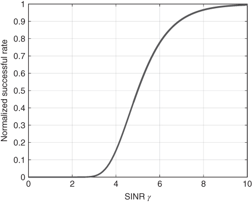
Figure 5.3 Illustration of  .
.
Combined with Eq. (5.1), the transmission delay from ![]() to
to ![]() is calculated as
is calculated as

Each sensor ![]() must finish the transmission of its aggregated data to
must finish the transmission of its aggregated data to ![]() before it transmits new data; therefore
before it transmits new data; therefore ![]() is bounded as follows:
is bounded as follows:

Let ![]() be the end‐to‐end delay for the data gathered by
be the end‐to‐end delay for the data gathered by ![]() to be successfully delivered to
to be successfully delivered to ![]() when each transmitter
when each transmitter ![]() always appends the aggregated data from
always appends the aggregated data from ![]() to the end of its own gathered data
to the end of its own gathered data ![]() . In this case,
. In this case, ![]() will suffer the longest end‐to‐end delay among all the data. Obviously, within
will suffer the longest end‐to‐end delay among all the data. Obviously, within ![]() , all data generated in a time period with respect to
, all data generated in a time period with respect to ![]() for all
for all ![]() will be delivered to
will be delivered to ![]() . Let
. Let ![]() ; in order to guarantee the successful delivery of all data in a time period, the system must meet the following requirement:
; in order to guarantee the successful delivery of all data in a time period, the system must meet the following requirement:
5.4 Proposed Power Allocation Schemes
In general, the monitoring data must be delivered to the control center within a short period of time. Therefore, the control center is not capable of gathering the real‐time status (e.g. ![]() ) of each sensor and computing a centralized optimal power allocation accordingly. Nonetheless, a centralized scheme can be feasible with the scenario described below. With an optimal power allocation predetermined, it is helpful to reduce the cost when deploying the sensors. Especially for sensors powered by green energy, solutions generated from the centralized schemes can be used to design the power supply equipment (e.g. solar panel size and battery capacity). In the rest of this section, we first propose several centralized power allocation schemes while taking into consideration the worst‐case scenario described below.
) of each sensor and computing a centralized optimal power allocation accordingly. Nonetheless, a centralized scheme can be feasible with the scenario described below. With an optimal power allocation predetermined, it is helpful to reduce the cost when deploying the sensors. Especially for sensors powered by green energy, solutions generated from the centralized schemes can be used to design the power supply equipment (e.g. solar panel size and battery capacity). In the rest of this section, we first propose several centralized power allocation schemes while taking into consideration the worst‐case scenario described below.
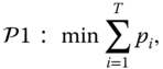
5.4.1 Minimizing Total Power Usage
Since the sensor nodes in the multihop wireless portion of the monitoring network are powered by green energy, it is important to reduce the power consumption of the sensors to lower the hardware cost. Therefore, the first centralized scheme ![]() is designed to minimize the total power consumption of the sensors that upload data to the same gateway (e.g.
is designed to minimize the total power consumption of the sensors that upload data to the same gateway (e.g. ![]() ). The scheme is shown below.
). The scheme is shown below.
subject to Eq. (5.5), Eq. (5.9), and Eq. (5.10),
.
However, there is no polynomial time algorithm to solve ![]() . We then relax some of the constraints. As indicated before, the end‐to‐end delay requirement
. We then relax some of the constraints. As indicated before, the end‐to‐end delay requirement ![]() is very small (e.g. 10 ms), however
is very small (e.g. 10 ms), however ![]() is relatively large (e.g. 1 s), so the constraint in Eq. (5.9) is implicitly satisfied in general. For the end‐to‐end delay, intuitively, if
is relatively large (e.g. 1 s), so the constraint in Eq. (5.9) is implicitly satisfied in general. For the end‐to‐end delay, intuitively, if ![]() gets higher, the solution to
gets higher, the solution to ![]() will be small, since each sensor is able to use less power to transmit and achieve the same delay requirement. Therefore, we relax the constraint shown in Eq. (5.10) to the following equation
will be small, since each sensor is able to use less power to transmit and achieve the same delay requirement. Therefore, we relax the constraint shown in Eq. (5.10) to the following equation
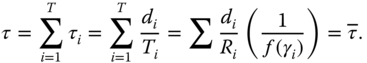
Note that ![]() is a constant in
is a constant in ![]() in the worst‐case scenario. Therefore, Eq. (5.12) is an equation with variables
in the worst‐case scenario. Therefore, Eq. (5.12) is an equation with variables ![]() . As discussed before,
. As discussed before, ![]() is an increasing function with respect to
is an increasing function with respect to ![]() , and
, and ![]() is also an increasing function with respect to
is also an increasing function with respect to ![]() if
if ![]() is given. Therefore, minimizing the total transmission power can be viewed as minimizing the summation of the normalized transmission data rate of each link. We write the relaxed problem into
is given. Therefore, minimizing the total transmission power can be viewed as minimizing the summation of the normalized transmission data rate of each link. We write the relaxed problem into ![]() as shown below with constraints.
as shown below with constraints.
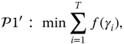
subject to Eq. (5.12) and

Constraint Eq. (5.14) is rewritten from Eq. (5.9) based on Eq. (5.1). It shows the lower bound of the normalized transmission rate of each link, below which the link would fail to deliver data before the transmission of new incoming data. Constraint Eq. (5.15) shows the upper bound of the normalized transmission rate of each link. The maximum SINR ![]() is achieved when
is achieved when ![]() . Since the objective is to minimize the summation of
. Since the objective is to minimize the summation of ![]() , we assume
, we assume ![]() is estimated when
is estimated when ![]() for all
for all ![]() . Now that
. Now that ![]() is simpler compared with
is simpler compared with ![]() , it is faster to find the optimal solution. The numerical results in the later section will demonstrate that. However, there is still no polynomial algorithm to achieve the optimal solution to
, it is faster to find the optimal solution. The numerical results in the later section will demonstrate that. However, there is still no polynomial algorithm to achieve the optimal solution to ![]() . Therefore, if the network size is large, then it will take much more computational time to get the solution.
. Therefore, if the network size is large, then it will take much more computational time to get the solution.
5.4.2 Maximizing Power Efficiency
In order to quickly converge to a solution, we propose a game theoretical scheme. A noncooperative game is formed as ![]() , where
, where ![]() is the set of sensors or players,
is the set of sensors or players, ![]() is the strategy set of each player, and
is the strategy set of each player, and ![]() is the corresponding utility. In traditional multiaccess wireless networks, the utility function is generally defined as the effective transmission rate over transmission power. However, such modeling does not work for the proposed monitoring network for two reasons. One is that the proposed monitoring network has a much more stringent delay requirement, while the traditional multiaccess wireless network is assumed to be more delay tolerant. The other reason is that the link requirement (e.g. SINR) cannot be simply assumed as uniform or fixed if an optimal (or suboptimal) solution is the goal.
is the corresponding utility. In traditional multiaccess wireless networks, the utility function is generally defined as the effective transmission rate over transmission power. However, such modeling does not work for the proposed monitoring network for two reasons. One is that the proposed monitoring network has a much more stringent delay requirement, while the traditional multiaccess wireless network is assumed to be more delay tolerant. The other reason is that the link requirement (e.g. SINR) cannot be simply assumed as uniform or fixed if an optimal (or suboptimal) solution is the goal.
In our proposed game for the monitoring network, two additional requirements must be satisfied for the utility function compared with the traditional one. One is that the maximizer of the utility function must be delay sensitive. Specifically, when ![]() is lower, the maximizer
is lower, the maximizer ![]() should be larger so that the effective transmission rate will be higher to adapt to the lower delay. The other requirement of the utility function is that the maximizer must respond to the dynamic traffic flow. That is to say, when
should be larger so that the effective transmission rate will be higher to adapt to the lower delay. The other requirement of the utility function is that the maximizer must respond to the dynamic traffic flow. That is to say, when ![]() is higher, the maximizer
is higher, the maximizer ![]() should be larger for a higher effective transmission rate. Therefore, we update the utility function for sensor
should be larger for a higher effective transmission rate. Therefore, we update the utility function for sensor ![]() into the one shown below,
into the one shown below,
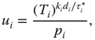
where ![]() is a weight factor and
is a weight factor and ![]() is the benchmark link delay, which can be the optimal solution to
is the benchmark link delay, which can be the optimal solution to ![]() or
or ![]() .
.
For each sensor ![]() , the goal is to maximize the utility, as shown in
, the goal is to maximize the utility, as shown in ![]() .
.
Figure 5.4 illustrates the unique maximizer ![]() and the impact of dynamic
and the impact of dynamic ![]() and benchmark
and benchmark ![]() on the maximizer. Obviously, when
on the maximizer. Obviously, when ![]() gets higher or
gets higher or ![]() gets lower, the maximizer
gets lower, the maximizer ![]() (if one uniquely exists) gets larger, and the corresponding effective transmission rate gets higher. Note that the unit of the utility function is not bit/joule.
(if one uniquely exists) gets larger, and the corresponding effective transmission rate gets higher. Note that the unit of the utility function is not bit/joule.
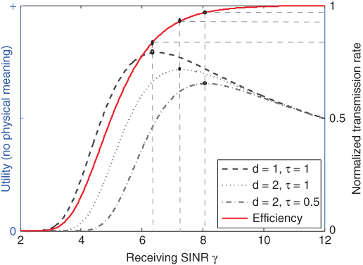
Figure 5.4 Illustration of the modified utility function.
Compared with ![]() and
and ![]() , the advantage of the proposed game theoretical scheme is that it is capable of finding the solution (the NE) quickly by finding
, the advantage of the proposed game theoretical scheme is that it is capable of finding the solution (the NE) quickly by finding ![]() for all
for all ![]() and then computing the corresponding power allocation
and then computing the corresponding power allocation ![]() for all
for all ![]() by solving a linear equation system. However, the disadvantage of the game theoretical scheme is that it must have the benchmark
by solving a linear equation system. However, the disadvantage of the game theoretical scheme is that it must have the benchmark ![]() , which is the optimal solution from a centralized power allocation scheme. Moreover, it must have a carefully chosen weight factor
, which is the optimal solution from a centralized power allocation scheme. Moreover, it must have a carefully chosen weight factor ![]() so that the constraint in Eq. (5.18) is satisfied.
so that the constraint in Eq. (5.18) is satisfied.
5.4.3 Uniform Delay
When the network size is large, it is time consuming to find the optimal solutions to ![]() and
and ![]() as benchmarks. Therefore, we further simplify the optimization problems so that a quick solution can be found. First, we assume that the delay for each link
as benchmarks. Therefore, we further simplify the optimization problems so that a quick solution can be found. First, we assume that the delay for each link ![]() is uniform, that is,
is uniform, that is, ![]() . Then the SINR
. Then the SINR ![]() for each link can be calculated from Eq. (5.3) and Eq. (5.8) as follows:
for each link can be calculated from Eq. (5.3) and Eq. (5.8) as follows:

Moreover, Eq. (5.2) can be represented as follows:

Therefore, with a given ![]() for all
for all ![]() , the set of power allocation
, the set of power allocation ![]() can be easily calculated by solving a linear equation system where the number of equations and the number of variables are both
can be easily calculated by solving a linear equation system where the number of equations and the number of variables are both ![]() . Note that the last link is required to have an effective transmission rate of
. Note that the last link is required to have an effective transmission rate of ![]() . Compared with the first link,
. Compared with the first link, ![]() could be several times higher than
could be several times higher than ![]() . However, since the packet from each sensor is small, and
. However, since the packet from each sensor is small, and ![]() is possibly several Kbps only, it is still reasonable for the monitoring network to apply equal delay in each transmission link.
is possibly several Kbps only, it is still reasonable for the monitoring network to apply equal delay in each transmission link.
5.4.4 Uniform Transmission Rate
If the data generated by a sensor node increases to some extent, a fixed link delay may no longer be a reasonable assumption. Alternatively, we can fix the transmission rate of each link, that is for all ![]() , as follows:
, as follows:

Without loss of generality, assume that ![]() , then
, then ![]() . From Eq. (5.10) we can get
. From Eq. (5.10) we can get
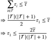
As stated before, Eq. (5.23) can be relaxed into equality, so that ![]() . With
. With ![]() and
and ![]() given,
given, ![]() can be easily computed and also
can be easily computed and also ![]() . Then the corresponding power allocation
. Then the corresponding power allocation ![]() can be found by solving the linear equation system Eq. (5.21).
can be found by solving the linear equation system Eq. (5.21).
5.5 Distributed Power Allocation Schemes
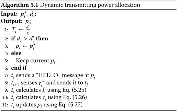
In field operations, centralized schemes are not applicable due to real‐time transmission of the monitoring network. Moreover, each sensor gathers data less frequently, and the data size is usually smaller than its maximum value in the worst‐case scenario. Therefore, although the radios must be active almost all the time, it is possible to have a distributed power allocation scheme based on dynamic data traffic to further reduce the power usage while allowing real‐time transmission. For each sensor ![]() , the most energy‐efficient power allocation is to use the minimum transmission power while delivering the data on time, that is,
, the most energy‐efficient power allocation is to use the minimum transmission power while delivering the data on time, that is,
subject to Eq. (5.5), Eq. (5.9), and Eq. (5.18).
However, without full knowledge of the network, it is impractical for ![]() to achieve an optimal solution. Moreover, the allocation of power must occur in a short time. Therefore, the goal for solving
to achieve an optimal solution. Moreover, the allocation of power must occur in a short time. Therefore, the goal for solving ![]() is to save as much power as possible while meeting the delay requirement at
is to save as much power as possible while meeting the delay requirement at ![]() .
.
Assume that the optimal power allocation ![]() and delay requirement
and delay requirement ![]() are predetermined based on the worst‐case scenario before the deployment of the network (e.g. the solution to
are predetermined based on the worst‐case scenario before the deployment of the network (e.g. the solution to ![]() ,
, ![]() , or
, or ![]() ). Note that the proposed distributed scheme is based on the dynamic data traffic. Therefore, sensor
). Note that the proposed distributed scheme is based on the dynamic data traffic. Therefore, sensor ![]() stores the length of the data previously sent as
stores the length of the data previously sent as ![]() for comparison. Before
for comparison. Before ![]() transmits data
transmits data ![]() ,
, ![]() checks its current
checks its current ![]() .
. ![]() first determines
first determines ![]() . Then if
. Then if ![]() , before
, before ![]() transmits the data, it sends a SINR request (a “HELLO” message) to
transmits the data, it sends a SINR request (a “HELLO” message) to ![]() at power
at power ![]() . At the same time,
. At the same time, ![]() senses
senses ![]() at its current status and replies with it to
at its current status and replies with it to ![]() . With given
. With given ![]() ,
, ![]() calculates the noise plus interference at
calculates the noise plus interference at ![]() as
as
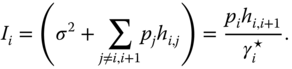
Then ![]() calculates adequate SINR as
calculates adequate SINR as
Obviously, ![]() . Then
. Then ![]() determines its current transmission power as
determines its current transmission power as
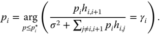
If ![]() , then
, then ![]() keeps transmitting at current
keeps transmitting at current ![]() and follows the process stated above to update its
and follows the process stated above to update its ![]() accordingly. The scheme is summarized in Algorithm 5.1.
accordingly. The scheme is summarized in Algorithm 5.1.
5.6 Numerical Results and A Case Study
In this section, we numerically analyze the proposed centralized schemes and conduct a case study to demonstrate the distributed scheme.
5.6.1 Simulation Settings
The studied monitoring network with transmission line model is shown in Figure 5.5. Without loss of generality, we assume that the length of the power line between two neighboring towers is ![]() km. However, the transmission towers are not necessarily installed in a straight line. To be more realistic, we assume that two neighboring towers have an angle of
km. However, the transmission towers are not necessarily installed in a straight line. To be more realistic, we assume that two neighboring towers have an angle of ![]() to the east. For simplicity, the elevation of the terrain is not considered in the settings, and the transmission line is assumed to be installed on a flat plain. Additionally, we assume that each
to the east. For simplicity, the elevation of the terrain is not considered in the settings, and the transmission line is assumed to be installed on a flat plain. Additionally, we assume that each ![]() is randomly chosen in
is randomly chosen in ![]() . Practically, the sensors are deployed on the selected towers instead of all towers. In the simulation setting, we assume that the sensors are mounted at every
. Practically, the sensors are deployed on the selected towers instead of all towers. In the simulation setting, we assume that the sensors are mounted at every ![]() towers. An example with
towers. An example with ![]() is illustrated in Figure 5.5. Note that the wireless transmission distance between
is illustrated in Figure 5.5. Note that the wireless transmission distance between ![]() and
and ![]() is generally shorter than
is generally shorter than ![]() .
.

Figure 5.5 Simulation setting for transmission line.
Without loss of generality, we assume that the multihop wireless sensor network (i.e. ![]() and
and ![]() ) is deployed on the towers with an end‐to‐end power line length of 10 kilometers. The rest of the setting are as follows: for all
) is deployed on the towers with an end‐to‐end power line length of 10 kilometers. The rest of the setting are as follows: for all ![]() , we set
, we set ![]() bit,
bit, ![]() Kbps,
Kbps, ![]() Hz. The end‐to‐end delay threshold
Hz. The end‐to‐end delay threshold ![]() ms, the processing gain
ms, the processing gain ![]() , the packet length
, the packet length ![]() bit, the physical layer transmission rate
bit, the physical layer transmission rate ![]() Mbps, and the transmission frequency
Mbps, and the transmission frequency ![]() MHz.
MHz.
5.6.2 Comparison of the Centralized Schemes
Assuming that the sensors operate in the f=230 MHz spectrum, it is practical for them to transmit over several kilometers. Therefore, without loss of generality, we evaluate ![]() from 1 to 10 if not otherwise specified. We first compare the results of
from 1 to 10 if not otherwise specified. We first compare the results of ![]() and
and ![]() with the following settings:
with the following settings:
- The towers are deployed with randomly chosen
 in the simulation setting.
 - In each comparison with
 sensors, we generate 100 random topologies.
 - For each generated topology, the power allocations are calculated by both
 and
and  .
. - The computation time is recorded.
The comparison is shown in Figure 5.6. Each result in the figure is an average value of the 100 solutions generated from 100 random topologies (excluding the largest and the smallest results for further accuracy) to the corresponding scheme. At we can see, solving ![]() for the optimal solution is much faster than solving
for the optimal solution is much faster than solving ![]() . However, even when
. However, even when ![]() is a small number (e.g.
is a small number (e.g. ![]() ), finding the optimal solution is too expensive to be applied for real‐time operation of the monitoring system.
), finding the optimal solution is too expensive to be applied for real‐time operation of the monitoring system.
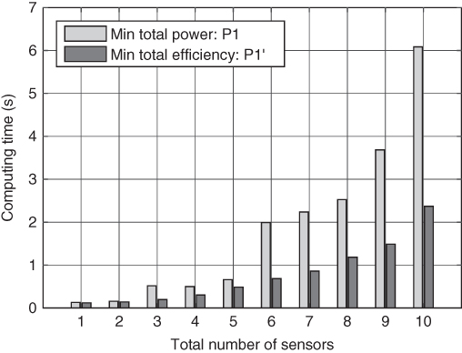
Figure 5.6 Computational time of  and
and  .
.
Second, we show the total transmission power for all the sensors with ![]() . In order to show the impact on the number of sensors more precisely, we place the transmission towers in a straight line (i.e.
. In order to show the impact on the number of sensors more precisely, we place the transmission towers in a straight line (i.e. ![]() ). As shown in Figure 5.7, the relaxed scheme
). As shown in Figure 5.7, the relaxed scheme ![]() has almost the same power allocation results as scheme
has almost the same power allocation results as scheme ![]() .
.

Figure 5.7 Total transmission power by solving  and
and  .
.
Third, we set ![]() and compare the results from different centralized schemes. Figure 5.8 shows the comparison of the normalized transmission efficiency of each sensor
and compare the results from different centralized schemes. Figure 5.8 shows the comparison of the normalized transmission efficiency of each sensor ![]() with different centralized schemes. We first calculate the solution to
with different centralized schemes. We first calculate the solution to ![]() . The solution is then used as the benchmark value for the game theoretical scheme. In the game theoretical scheme, the weight factor is set as
. The solution is then used as the benchmark value for the game theoretical scheme. In the game theoretical scheme, the weight factor is set as ![]() for all
for all ![]() . As we can see,
. As we can see, ![]() and
and ![]() have results close to each other, which indicates that the relaxation of
have results close to each other, which indicates that the relaxation of ![]() remains a good approximation. The game theoretical scheme also has a result close to that of
remains a good approximation. The game theoretical scheme also has a result close to that of ![]() , because it is based on the benchmark setting from
, because it is based on the benchmark setting from ![]() . The equal link delay scheme requires linearly increasing transmission efficiency as the link gets closer to the gateway, because the amount of data increases linearly as it is uploaded to the gateway. On the other hand, the equal transmission rate scheme results in a flat transmission efficiency.
. The equal link delay scheme requires linearly increasing transmission efficiency as the link gets closer to the gateway, because the amount of data increases linearly as it is uploaded to the gateway. On the other hand, the equal transmission rate scheme results in a flat transmission efficiency.
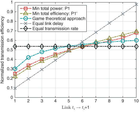
Figure 5.8 Normalized transmission efficiency of each sensor.
Figure 5.9 shows the corresponding SINR ![]() for all
for all ![]() of the centralized schemes. Note that the last link requires a much higher SINR in the scheme with equal link delay; therefore the last sensor requires a much larger power supply component, which will make the deployment more complicated.
of the centralized schemes. Note that the last link requires a much higher SINR in the scheme with equal link delay; therefore the last sensor requires a much larger power supply component, which will make the deployment more complicated.

Figure 5.9 SINR of each sensor.
Figure 5.10 shows the delay ![]() for each link
for each link ![]() achieved by the different centralized schemes. In comparison, all the schemes (except for the equal link delay one) have an increasing link delay as the sensors get closer to the gateway, because of the increase in aggregated data. The end‐to‐end delays for all the centralized schemes are the same as
achieved by the different centralized schemes. In comparison, all the schemes (except for the equal link delay one) have an increasing link delay as the sensors get closer to the gateway, because of the increase in aggregated data. The end‐to‐end delays for all the centralized schemes are the same as ![]() . The end‐to‐end delay for the game theoretical scheme is
. The end‐to‐end delay for the game theoretical scheme is ![]() . The game theoretical scheme achieves a slight advantage because of its slightly higher transmission power.
. The game theoretical scheme achieves a slight advantage because of its slightly higher transmission power.
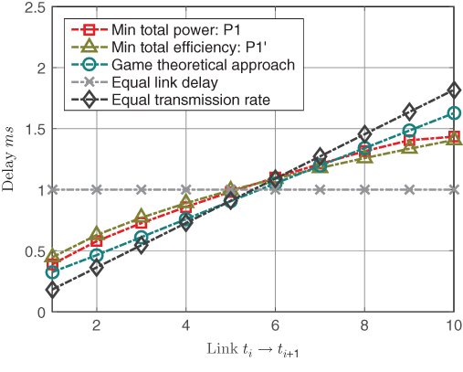
Figure 5.10 Delay of each link.
Figure 5.11 shows results of total transmission power achieved by different schemes. Compared to the optimal solution generated by ![]() ,
, ![]() and game theoretical scheme have close‐to‐optimal results. For practical purpose, the equal transmission rate scheme is recommended over the equal delay scheme, since its results are closer to optimal.
and game theoretical scheme have close‐to‐optimal results. For practical purpose, the equal transmission rate scheme is recommended over the equal delay scheme, since its results are closer to optimal.
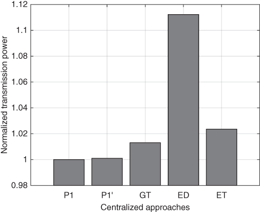
Figure 5.11 Comparison of normalized transmission power.
5.6.3 Case Study
In the case study, the transmission line is randomly deployed following the previous setting with ![]() sensors. It is then fixed throughout the discussion. At sensor
sensors. It is then fixed throughout the discussion. At sensor ![]() , its monitoring data
, its monitoring data ![]() is assumed to be generated at a random rate
is assumed to be generated at a random rate ![]() , and the gathered data
, and the gathered data ![]() ,
, ![]() . We first show the adaptive power allocation for sensor
. We first show the adaptive power allocation for sensor ![]() in 20 time slots (
in 20 time slots (![]() ) to demonstrate its adaptability to the dynamic traffic in Figure 5.12. In Figure 5.13, we show the link delay
) to demonstrate its adaptability to the dynamic traffic in Figure 5.12. In Figure 5.13, we show the link delay ![]() of link
of link ![]() and the corresponding end‐to‐end delay
and the corresponding end‐to‐end delay ![]() . Note that the end‐to‐end delay is always below the required
. Note that the end‐to‐end delay is always below the required ![]() ms; therefore, the distributed power allocation scheme is valid for practical operations.
ms; therefore, the distributed power allocation scheme is valid for practical operations.
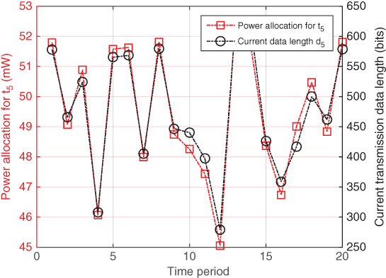
Figure 5.12 Dynamic power allocation for  .
.
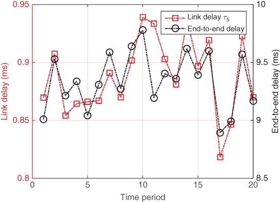
Figure 5.13 Corresponding  and
and  .
.
5.7 Summary
In this chapter, we designed and analyzed a wireless sensor–based monitoring network for the transmission lines in the smart gird. Specifically, we studied the power allocation for the wireless multihop sensor network between two OPGW gateways. In order to set the power allocation benchmark for the design of the wireless sensors, we proposed several centralized schemes, including two optimization problems, ![]() and
and ![]() , that minimize the total power consumption, a game theoretical scheme, and two relaxed schemes that converge to solutions quickly in a large scale network. Based on the benchmark set by the centralized schemes, we also proposed a distributed power allocation scheme for field operations with dynamic traffic. The simulation results showed that finding solutions to both
, that minimize the total power consumption, a game theoretical scheme, and two relaxed schemes that converge to solutions quickly in a large scale network. Based on the benchmark set by the centralized schemes, we also proposed a distributed power allocation scheme for field operations with dynamic traffic. The simulation results showed that finding solutions to both ![]() and
and ![]() consumes too much time for field operations. The case study demonstrated that considering field operations with dynamic traffic, our proposed distributed power allocation scheme can satisfy the end‐to‐end delay requirement and is more energy efficient than the benchmark. Detailed monitoring technologies for each comprehensive sensor node based on the upgraded monitoring network require future research.
consumes too much time for field operations. The case study demonstrated that considering field operations with dynamic traffic, our proposed distributed power allocation scheme can satisfy the end‐to‐end delay requirement and is more energy efficient than the benchmark. Detailed monitoring technologies for each comprehensive sensor node based on the upgraded monitoring network require future research.