
15
Microelectromechanical systems integrating motion and displacement sensors
Abstract
The purpose of this chapter is to describe the working principle of the microelectromechanical systems (MEMS) devices used in motion sensors and to consider their level of sophistication, performance limits, and future evolution. The integration of a multiparameter sensor in a single unit can increase the smartness of the device and enables the implementation of new functionalities in existing electronic systems. MEMS accelerometers, gyroscopes, and magnetometers are discussed in detail, as they represent the core devices for the development of a high-precision inertial measurement unit. At the end of the chapter, consideration is given to the evolution of these units integrating new MEMS devices for added functionalities, such as pressure sensing or proximity measurements.
Keywords
Accelerometers; Barometers; Gyroscopes; Inertial measurement units; Magnetometers; MEMS motion sensors; Navigation
15.1. Introduction
A smart motion sensor is, in its simplest form, a single unit capable of providing information on linear and rotational displacements for all the three possible axes of motion and possibly also initial orientation with respect to a reference system. This kind of sensor can be presently made using microelectromechanical systems (MEMS) technology for the transducing part, often combined with an application-specific integrated circuit (ASIC) that implements the control and readout electronics and with a microprocessor that implements a fusion of raw data to give added value to the combination of all different measurements. The main purposes of this chapter are to present the basic working principle of the MEMS devices used to implement this unit, to describe typical and advanced driving and sensing methods, and to explore the evolution of their smartness in a near future where concepts such as Internet of things and ubiquitous sensors are expected to see their dawn.
The basic devices that make up a motion sensor unit, also referred to as an inertial measurement unit (IMU), are the accelerometer and the gyroscope; the accelerometer is used to measure linear motion, and the gyroscope is used to measure rotational motion. These devices have been used for decades, but the extensive spread of their use since the turn of the millennium is because of the research and industrial progress obtained in MEMS technology. First, the possibility of implementing such devices in very small dimensions and with ultralow power consumption was very attractive and led to the development of primitive MEMS devices for single-axis, single-parameter measurements (Boser and Howe, 1996; Kempe, 2011). But it is only in the last few years (since 2009) that the smartness obtained from the combination of multi-axes and multiparameter MEMS units has opened new fields of application for IMUs and contributed to the integration of new functionalities in existing electronic systems. This combination of sensors gives advantages in terms of both cost production for the MEMS supplier and solutions offered to the system integrator.
In particular, consumer electronics has profited enormously from this development and now triaxial accelerometers and gyroscopes can be found in game controllers, sport equipment, notebooks and netbooks, portable media players, digital still cameras, and mobile phones. Actually, it can be stated that most of the smartness of a smartphone is given by the sensors embedded in it. Among the other sectors, the automotive industry still holds almost the same market share as consumer electronics, with massive use in airbags, electronic stability control, and tire pressure monitoring systems. Inertial sensors with higher performance requirements can be found also in the medical, industrial, aerospace, and military markets (e.g., medical human motion analysis, land transportation systems, oil drilling and exploration, civil and military aviation, and unmanned vehicles). Another killer application, which is promising to bring high-performance inertial sensors also in the consumer market, is pedestrian navigation, with very attractive indoor navigation features given by the fusion of inertial sensors data and signals provided by landmark beacons (e.g., wi-fi spots, etc.). On the whole, according to Mounier et al. (2016), inertial sensors are still driving the MEMS market. On the whole (including stand-alone accelerometers, gyroscopes, barometers and magnetometers, as well as inertial combos), their market will grow from $4.6 billion in 2016 to $9 billion by 2021, with in particular a compound annual growth rate for combos only of about 10%. Interestingly, the single sensor price will continuously drop because of increase of requests and size scaling (accelerometers already cost, on average, 0.14$ only!).
The state-of-the-art of IMUs made with MEMS sensors is only represented by the “6-axis” (or “6-degrees-of-freedom—DOF”) units, integrating 3-axial accelerometers and gyroscopes made in the same process (examples of which can be found in Invensense, 2016; ST Microelectronics, 2013). Further smartness and a greater number of features could be obtained if the IMUs were also capable of measuring the absolute orientation of the object that incorporates it. With this added feature, heading, navigation, compass, and dead-reckoning applications could be implemented because the loss of absolute orientation over time (due to thermal drifts mainly), which is typical of 6-DOF IMUs, could be corrected. Absolute orientation can be obtained using a magnetometer or digital compass. At the state-of-the-art, 9-DOF systems integrate non-MEMS magnetic field sensors (see, e.g., ST Microelectronics, 2014a,b); clearly, the integration of magnetometers in a MEMS process would be very advantageous both from a production cost perspective and for the further downsizing of the motion sensor. Demonstrations of such devices have been given in the scientific literature (Emmerich and Schofthaler, 2000; Langfelder et al., 2014; Minotti et al., 2015; Laghi et al., 2016) and it is likely that all-MEMS 9-DOF IMUs will soon enter the market. In an alternative perspective, micromachining technologies can help improving the performance of existing non-MEMS sensors embedding magnetic materials, e.g., in Lai et al. (2015).
In the following section, details will be given regarding the structure and working principle of MEMS accelerometers, gyroscopes, and magnetometers; consideration will be given to various topologies and the focus will be on their specifications for consumer and automotive applications.
The operation of all of the MEMS devices described is governed by means of suitable electronics, generally embedded in an ASIC. Even if the production of the MEMS and the integrated circuit on the same ASIC is possible (Geen et al., 2002), the use of separate processes allows a better optimization of their respective performances, albeit at the cost of a larger area. This was confirmed in the last years by the dramatic scaling on MEMS size on one side and on ASIC power consumption on the other side, while keeping or even improving noise and full-scale range (FSR) performance. The waste of area required by the combination of the MEMS and the ASICs will be considerably reduced with the advent of smart interconnections such as through silicon vias (TSV, see, e.g., Fischer et al., 2011) or the so-called Nasiri process (used, e.g., in Invensense, 2016).
For a single device, the ASIC not only transduces the information regarding the quantity to be measured into an electrical signal and operates its conversion into the digital domain but also provides an active function in the transduction principle (for instance, it keeps the device in oscillation for vibratory sensors, as will be detailed in the following section). The important point is that the choice of the driving and readout architecture of a MEMS device has a strong interdependence on the mechanical architecture, and both have an impact on the performance of a device—typically described in terms of sensitivity, resolution, power consumption, FSR, and operation bandwidth. When deriving the mathematical equations for these parameters, one should take into account these considerations to draw sound and valid conclusions.
In the next section, attention will be given to capacitive motion sensors (i.e., to devices where a change in the quantity to be measured results in a change of a suitably designed capacitance). The electronic readout then turns into a capacitance readout. This is the solution mostly widely used by MEMS sellers as it relies on a simple process that does not involve piezoelectric, piezoresistive, or magnetic materials.
As a consequence, the mechanical sensitivity is defined here for every device as the capacitance variation per unitary variation of the quantity to be measured. Electronic sensitivity takes into account the readout circuit and will be expressed in terms of voltage variation at the output per unitary variation of the quantity to be measured. Other important parameters that must be taken into consideration during the project of a device are the minimum measurable signal, or resolution, which corresponds to the overall system noise and is expressed in the same unit of the quantity to be sensed; the full scale, corresponding to the maximum measurable variation; and, finally, the operation bandwidth, which corresponds to the maximum frequency of interest during the measurement.
As a numerical reference, Table 15.1 summarizes the state-of-the-art specifications for consumer applications.

15.2. Technical description of MEMS motion sensors: MEMS accelerometer
MEMS accelerometers are used to sense linear accelerations in the x, y, and z directions. This section deals with the main issues faced by MEMS designers during the dimensioning of these devices. Fig. 15.1 presents the schematic of a uniaxial MEMS accelerometer with capacitive readout (Biswas et al., 2007; Boser and Howe, 1996; Langfelder et al., 2011). The device comprises a seismic mass, constrained to move only in the x-direction by a set of springs anchored to the substrate. A set of capacitive parallel-plate differential cells is used to sense the displacements of the seismic mass. Each capacitive cell comprises a moving part (rotor) and two electrodes fixed to the substrate (stators).
15.2.1. Mechanical model
The 1D movement of the seismic mass can be described by the well-known motion equation:
where m is the seismic mass value, b the damping coefficient, km the mechanical elastic stiffness of the springs along the x-direction, and Fext the sum of external forces acting on the device. When designing MEMS devices, it is useful to study certain aspects regarding frequency. By transforming Eq. (15.1) by means of Laplace, the transfer function between an external force and the corresponding displacement can be written as:
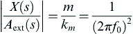
In Eq. (15.2),  is the mechanical resonance frequency of the device and Q = ω0m/b its quality factor. These two parameters are perhaps the most important to deal with when designing a MEMS accelerometer, as will be shown shortly. Fig. 15.2 reports examples of the transfer function modulus of an accelerometer with an elastic stiffness of 2 N/m; values around this one are typical of consumer applications to obtain resonance frequencies around a few kHz in low footprint dimensions (e.g., 400 μm × 400 μm). The plot is characterized by a flat response from the low-frequency range until the resonance frequency is reached, governed by the relation:
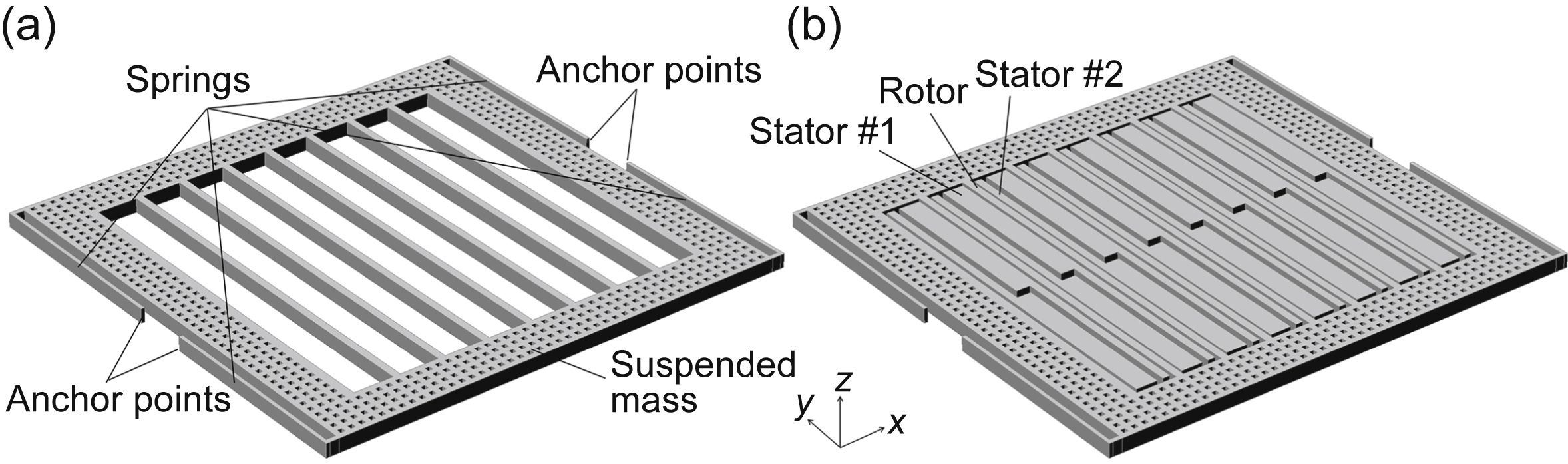
Figure 15.1 Schematic illustration of a uniaxial microelectromechanical systems accelerometer. (a) View of the rectangular suspended mass enclosing the space for the sensing capacitors and (b) view of the full device with the differential stators.
Beyond the point at which resonance occurs, the frequency response decreases as a transfer function with two poles (−40 dB/decade). Therefore, the range [0 < f < f0] represents the (maximum) mechanical bandwidth of the accelerometer, usually identified with the resonance frequency BW = f0. For consumer and automotive applications, the frequencies of interest are lower than 100–300 Hz, so typically the device bandwidth is set around 1–3 kHz (one order of magnitude above). By substituting Fext = maext in Eq. (15.3), where aext is the external acceleration, we can have a better understanding of the importance of the resonance frequency value:
 (15.4)
Eq. (15.4) shows that, given an external acceleration, the displacement of the seismic mass depends on the ratio of the mass and the elastic stiffness and not on their separate values alone. A common mistake is to assume that a larger mass leads to a more sensitive accelerometer; as shown in Eq. (15.4), this is ultimately not true. In conclusion, by setting the resonance frequency of the accelerometer (mainly considering the bandwidth requirements), one sets the relation between the displacement and the external acceleration. A large mechanical gain implies small bandwidths, indicating a gain-bandwidth trade-off.
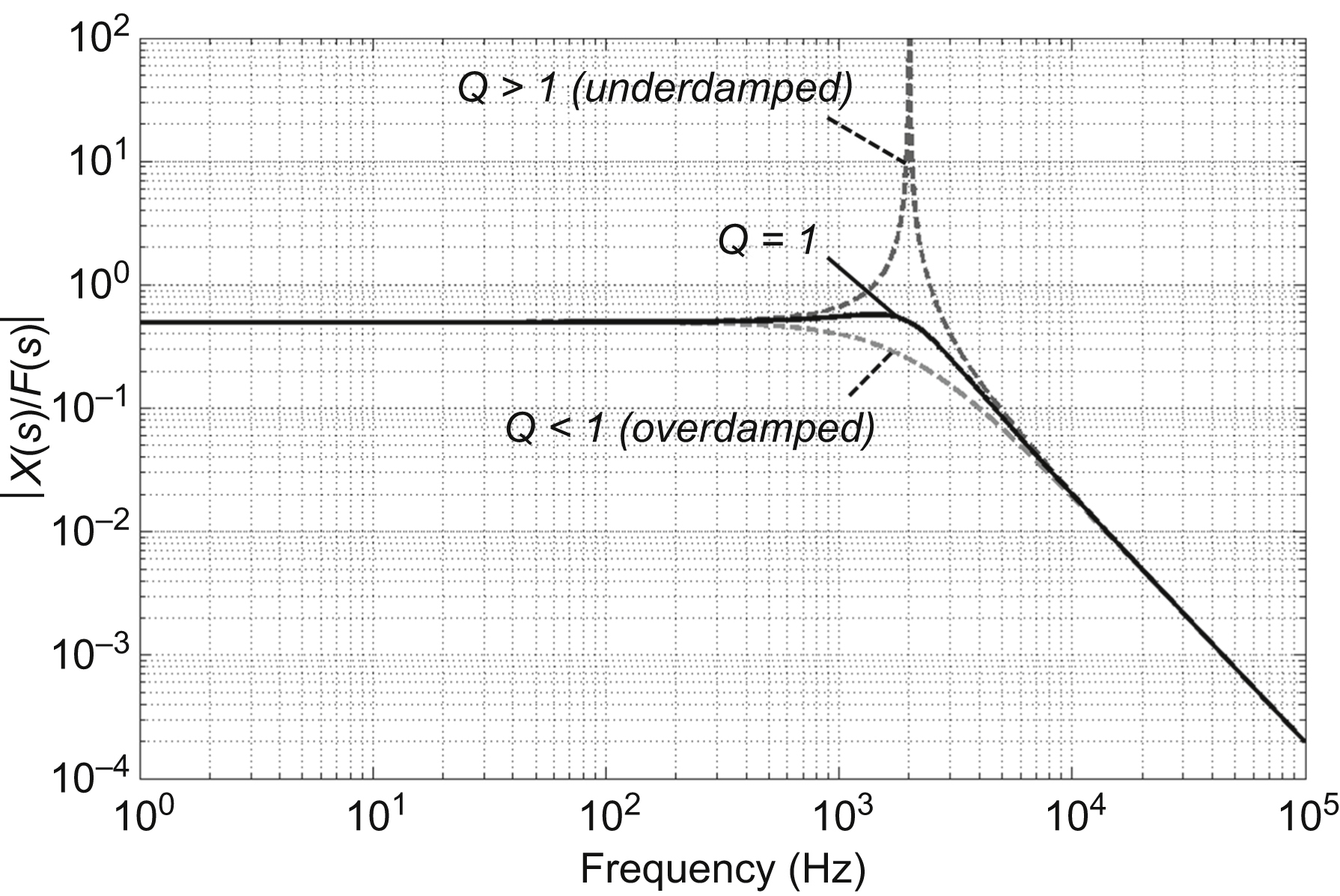
Figure 15.2 Modulus of the transfer function between the external force and the displacement of a uniaxial microelectromechanical systems accelerometer for different values of the quality factor.
A further relevant fact can be observed in Fig. 15.2; in the correspondence of f0, the modulus of the transfer function can either decrease smoothly or show a peak, depending on the quality factor value Q. The response is identified as overdamped where Q < 0.5 and as underdamped where Q > 0.5. This value depends greatly on the pressure set inside the package hosting the device during the process; capacitive accelerometers are packaged in such a range that the quality factor Q is typically lower than or around 1, to ensure an overdamped response from the device, without peaks in the transfer function, and simultaneously without lowering the bandwidth, which occurs for too overdamped configurations (due to pole splitting). Indeed, a peak would result in large unwanted oscillations of the seismic mass in the event of external vibrations around f0 or in case of shocks. Let us consider, for instance, mobile applications, where the accelerometer can be mounted adjacent to a loudspeaker emitting a signal in the audio bandwidth (20 Hz–20 kHz), or automotive applications, where the sensor operates in an acoustically and mechanically harsh environment (Dean et al., 2007); in both situations, any tones around f0 would lead to a corrupted signal from the accelerometer.
An exception to the use of quality factors around unity occurs for those applications where noise requirements are stringent, such as in seismic applications.
15.2.2. Differential capacitive sensing
Differential parallel-plate capacitive architecture represents the state-of-the-art of readout techniques currently integrated in most accelerometers for both the consumer and the automotive markets. The main advantage of this topology over other approaches (e.g., comb fingers capacitance) is its unbeaten high sensitivity in relation to the area occupation. This topology comprises an array of moving electrodes (rotors) attached to the suspended mass and by two groups of fixed electrodes (stators), forming two MEMS capacitors C1 and C2 (see Fig. 15.1(b)) defined as:
where ε0 is the vacuum permittivity, A is the facing area of the plates, x0 is the gap between each stator and the rotor in the rest position, and x is the displacement of the rotor from its rest position. Often, to keep the area required for the device to a minimum, these capacitances are embedded as several differential capacitive cells in the central part of the device (see again Fig. 15.1(b)). A positive displacement of the seismic mass (and thus of the rotors) in the x-direction causes the decrease of C1 and the increase of C2. Under the assumption of small displacements x ≪ x0, the differential capacitance variation can be linearized as follows:
where C0 being the capacitance at rest between the stator and the rotor. The relation between the capacitance variation and the displacement can be thus approximated as linear for small displacements. A common approach is to design the device such that its dimensions—and thus the mechanical resonance frequency (see Eq. 15.4) and the capacitances—ensure the maximum accepted linearity error over the desired FSR. Typical values of the FSR are in the range ±2 to ±12 g. As a numerical example, a 1% nonlinearity error is obtained for a displacement x corresponding to 1/10 of the gap value g. So in the design phase, assuming a gap at rest of 2 μm, the resonance will be set to such a value that the displacement obtained from Eq. (15.4) for an acceleration corresponding to the FSR matches 1/10 of the gap, i.e., 200 nm.
By substituting Eq. (15.4) into Eq. (15.6), we can define what is identified here as the mechanical sensitivity, defined as the differential capacitance variation ΔC per variation of external acceleration:
where the external acceleration has been substituted by its corresponding number of g-units, Ng = aext/9.8 m/s2. The defined mechanical sensitivity is thus expressed in Farad per g-units (F/g).
15.2.3. Thermomechanical noise
The minimum acceleration signal that can be measured is ultimately limited by noise sources, either intrinsic in the device or related to the readout electronics. Regarding intrinsic noise sources, the main contribution is associated with mechanical energy losses (damping). In particular, fluid damping generates thermomechanical fluctuations of the rotor caused by the Brownian motion of the gas particles inside the device package. These particles hit the movable elements of the sensor causing a sort of stochastic trembling. The phenomenon is well known in the literature (Tsai and Fedder, 2005), where the noise power density of the force acting on the seismic mass as a consequence of this Brownian noise is reported as:
In Eq. (15.8), kB is the Boltzmann's constant and T is the absolute temperature. This spectral density has a frequency behavior similar to that of white noise and it is expressed in N2/Hz. By using the relation between the external acceleration and the corresponding force, another important parameter characterizing the performance of a MEMS accelerometer can be obtained, the acceleration noise power density:
expressed in g2/Hz. The minimum detectable acceleration, or the sensor resolution, is defined as:
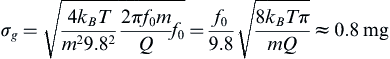
In general, the resolution required for the applications considered here is in the order of 1 mg. To give a numerical example, let us consider the following typical parameters for an accelerometer: a seismic mass m = 5 × 10⁻⁹ kg, a resonance frequency f0 = 2.5 kHz, and a quality factor Q ∼ 2. We can evaluate the intrinsic resolution of the accelerometer on its entire bandwidth as:
 (15.11)
Note once more that a low f0 has, in principle, a positive impact on the performance; nevertheless, apart from limiting the device bandwidth, the design of an accelerometer with a low f0, obtained by decreasing the stiffness k, can lead to the well-known “pull-in” phenomenon, as will be shown, and to consequent dangerous adhesion phenomena.
The relevant parameters for the design of a MEMS accelerometer have been identified and described in this section: the mechanical bandwidth, the sensitivity of the device, and the acceleration noise density. The next step is to turn the variation in capacitance into an electrical signal from the MEMS.
15.2.4. Electronic readout
The electronic readout circuit converts the information on the variation in capacitance due to an external acceleration into a voltage signal. In this section, we will present the basic configuration for the readout of capacitive MEMS motion sensors, the charge preamplifier. Let us consider the electrical scheme represented in Fig. 15.3(a), where the capacitive accelerometer is represented as its simplified electrical equivalent, a moving electrode between two fixed electrodes.
The moving plate is connected to the virtual ground of the charge preamplifier, formed by an operational amplifier with a feedback capacitance Cf. The stators #1 and #2 are biased at a voltage +V0 and −V0, respectively. In this configuration the rotor is thus kept at a fixed voltage (ground, in this example) with a constant potential across the two capacitances. The expressions of the electrical charges on the two capacitances at rest can be written as:
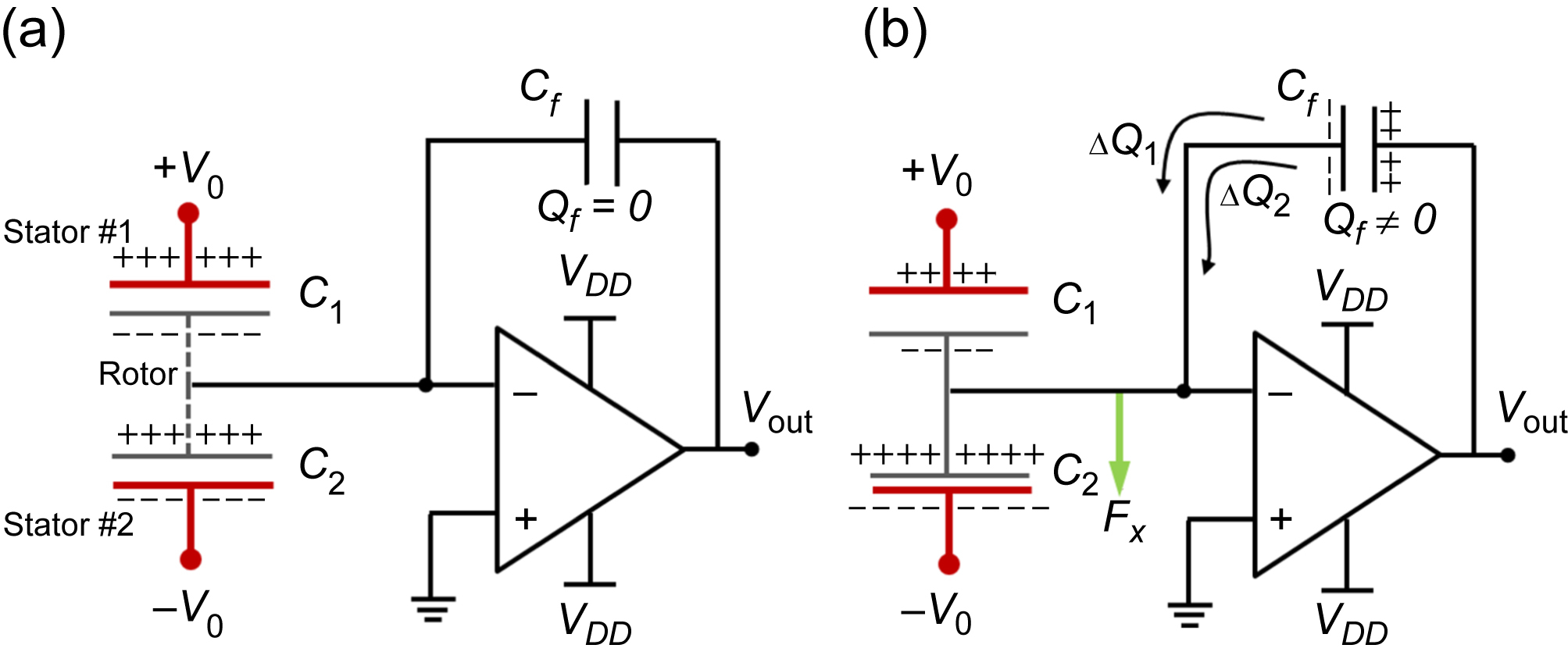
Figure 15.3 Schematic of the readout for a microelectromechanical systems accelerometer. (a) The virtual ground of a charge amplifier is connected to the rotor of the accelerometer. The overall charge on the rotor is nominally null for C1(x = 0) = C2(x = 0) and (b) a displacement of the seismic mass determines a charge on the feedback capacitance, which results in a variation of the output voltage.
and thus the net charge on the rotor node is null. Referring to Fig. 15.3(b), let us suppose that the rotor moves in the x-direction because of an external acceleration, causing a differential capacitance change. As a consequence, the charge on C1 decreases while the charge on C2 increases to satisfy Eq. (15.12). The charge variation on each capacitance with respect to the initial charge is simply:
These charges can be provided to the MEMS by the charge preamplifier through its feedback network, as shown in Fig. 15.3(b). In particular, the total provided charge is the sum of the two charge variations. Considering the expression for the differential capacitance variation ΔC derived in Eq. (15.6):
This charge causes a variation of the output voltage of the preamplifier equal to:
which give us the relationship between the preamplifier output voltage and the rotor (seismic mass) displacement. The factor 1/Cf can be considered to be the gain of the charge amplifier and should be chosen to have the maximum allowed output voltage change for an input number Ng of g-units corresponding to the FSR.
There is an important observation to be made at this point: the biasing voltages ±V0, essential for the capacitance readout, are also sources of electrostatic forces acting on the seismic mass and altering its mechanical behavior with respect to what described in Section 15.2.1. Each stator indeed exerts an attractive force on the seismic mass that can be written as:
By summing these two forces, the total electrostatic force acting on the seismic mass—under the assumption of small displacements—can be obtained:
Interestingly, it transpires that this electrostatic force appears proportional to the displacement x and it is therefore possible to define the term ke, which is generally referred to, in the literature, as the electrical equivalent stiffness. The mechanical behavior of the accelerometer when embedded in a readout design such as that presented in Fig. 15.3 can be therefore described by adding the electrostatic force term of Eq. (15.17) in the motion equation:
The presence of the electrical term ke has relevant effects on the behavior of the seismic mass. One of them is the pull-in phenomenon (Nielson and Barbastathis, 2006), a mechanical instability that arises when the electrical stiffness equals the mechanical stiffness. As detailed in the literature, apart from limiting the maximum signal bandwidth, the choice of a small value of km to increase the sensitivity by decreasing f0 also leads to accelerometers with a small equivalent stiffness (km − ke). In particular, in the limiting condition where km = ke the device loses its stable equilibrium point. The circuit presented is a simplified architecture of a typical electronic readout design. More complicated readout circuits, usually exploiting switching capacitor configurations and/or feedback circuits, can be used to decrease the power dissipated by the electronics and to solve the problems related to the pull-in instability (Langfelder et al., 2011; Seeger and Boser, 2003).
The change in the effective stiffness of the system leads also to the definition of an equivalent resonance frequency:
It is worth noting that the effect of the electrical stiffness is always to diminish the total system stiffness, thus decreasing the resonance frequency. This effect has to be taken into account both for the choice of the bandwidth for a device and for the evaluation of the sensitivity, which can be obtained by substituting Eq. (15.4) in Eq. (15.16) and by deriving with respect to external acceleration in g-units:
Eq. (15.20) represents the electronic sensitivity, expressed in V/g. Usually, the device and the readout electronics are of dimensions such that the maximum voltage output allowed by the electronics ΔVout,max is obtained with an acceleration signal corresponding to the target FSR of the accelerometer, ΔNg,max.
The conclusions drawn here for in-plane accelerometers can be extended to out-of-plane (tilting) devices (Lemkin et al., 1997; Selvakumar and Najafi, 1998) to implement a three-axis acceleration measurement unit.
15.2.5. Frequency-modulated accelerometers
The scalability of a capacitive accelerometer is somewhat limited by the pull-in phenomenon. Indeed, the bare scaling of the overall dimensions would lead to a lower mass and thus to a higher resonance frequency, in turn, leading to a lower sensitivity (see Eqs. 15.4 and 15.7). To compensate for this change, one would design a device with a smaller mechanical stiffness km. This is, ultimately, in contrast with Eq. (15.18), which states that a low mechanical stiffness can lead to an accelerometer with an overall null or negative equivalent stiffness (km − ke), thus being mechanically unstable when biased through a readout circuit such as the one described above.
Other issues of state-of-the-art accelerometers are represented by mechanical offset and its drift with temperature and or humidity.
One possible solution to above-mentioned problems, and one which has been given much attention in the scientific literature, is the frequency-modulated (FM) (or resonant) accelerometer concept (Aikele et al., 2001; Roessig et al., 1997; Seshia et al., 2002a,b; Zotov et al., 2015; Zou and Seshia, 2015). In this approach, an external acceleration acting on the MEMS device does not determine a change in a parallel-plate capacitance but, rather, a change in the resonance frequency of a suitably designed resonating element. A simple schematic of the working principle of such a device is shown in Fig. 15.4(a). The device comprises an inertial mass suspended between a pair of suitably designed springs and two suspended beams, each having the same nominal resonance frequency at rest, fbeam,1 = fbeam,2. For an external acceleration aext, the suspended mass is subject to the displacement given by Eq. (15.4). This displacement determines a differential stress on the beams and thus a differential change in their resonance frequencies. It has been shown (Comi et al., 2010) that for small stresses the differential frequency change Δfbeam = (fbeam,1 − fbeam,2) can be linearized and it is in first approximation proportional to the external acceleration. In alternative configurations, the external acceleration can determine a change in the equivalent electrical stiffness instead of the mechanical stiffness (Comi et al., 2016; Zotov et al., 2015). This enables the design of FM accelerometers also for out-of-plane sensing.
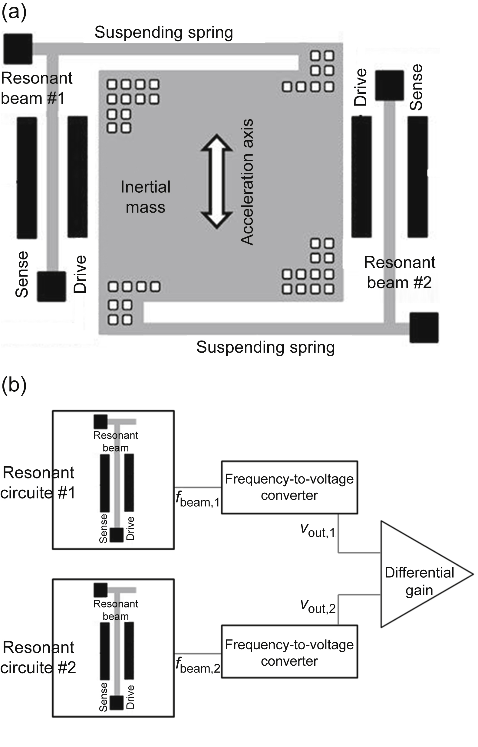
Figure 15.4 (a) Schematic structure of a resonant accelerometer: an acceleration acting on the inertial mass determines a differential stress on two beams, held in oscillation through capacitive driving and sensing electrodes (in black); (b) schematic representation of the readout electronics, including two oscillators, two frequency-to-voltage converters and a differential gain stage.
The readout electronics can be implemented as depicted in Fig. 15.4(b); the beams are held in oscillation through suitable driving circuits (Tocchio et al., 2012; Langfelder et al., 2014). The frequencies of each oscillator output are converted to voltage stages and their difference is computed through a final differential gain stage. An output signal proportional to the external acceleration is then obtained with specific frequency-to-digital conversion topologies (Izyumin et al., 2015).
Apart from the immunity to pull-in, which guarantees a high dynamic range, one of the advantages of this approach is that is takes up less room because of the small sensing elements (the two beams), unlike the array of stators required in the parallel-plate approach (see Fig. 15.1). The largest drawbacks are in that a precise matching between the nominal frequencies of the two resonators is required to minimize thermal drifts and in that a low pressure is required to guarantee a good quality factor for the resonating beams. A high-quality factor is mandatory prerequisite to minimize phase noise and power dissipation within the two oscillating circuits. This low pressure requirement, however, conflicts with the need for the quality factor of the suspended mass to be kept low, to guarantee operation within the required bandwidth. This presently represents the main limitation to the deployment of this kind of device within the application considered in this chapter.
15.3. Microelectromechanical systems gyroscope
A gyroscope is a device used to measure the angular rate around a certain axis of rotation. Like other kinds of gyroscopes, MEMS gyroscopes also rely on the physical principle of the Coriolis force to perform the measurement. An object with a certain velocity v and an angular rate Ω around an axis orthogonal to the vector v is subject to Coriolis acceleration:
A corresponding Coriolis force acts on the object with a direction orthogonal to the plane of both the axis of rotation and the direction of velocity and with the following modulus:
It is therefore important to ensure that the Coriolis force manifests only in presence of a velocity v; this immediately suggests that a MEMS gyroscope will also need to embed a driving section to apply a known velocity to a suspended mass. This is one major design difference with respect to the design of an accelerometer from a system-level point of view.
15.3.1. Working principle
An example of a MEMS gyroscope for the measurement of the angular rate along the z-axis is shown in Fig. 15.5 (Neul et al., 2007; Sharma et al., 2007; Kempe, 2011). The device is formed by an external frame (the drive frame) suspended in such a way that it is free to move in the x-direction and is strongly constrained in the y-direction. Together with the fixed components, this frame forms two comb finger capacitances that are used to apply the velocity v, as will be described. A set of suitably designed springs couples the drive frame to a second suspended frame (the Coriolis frame) in such a way that it is dragged by the drive frame along the x-direction but is also free to move in the y-direction. If a rotation around the z-axis occurs while the two masses are kept in oscillation with a velocity v, a Coriolis force pushes both the masses in the y-direction. The drive frame—constrained by the springs—does not move as a result of this force; the Coriolis frame is, instead, subject to a displacement that causes a differential capacitance variation with respect to the stators designed in the same differential configuration as that seen for the accelerometers. The drive frame is usually kept in oscillation at the resonance frequency fD of the drive mode. This allows the exploitation of the velocity amplification given by the quality factor QD in the drive direction, as described in the previous section. To obtain a large value of QD, the electrostatic actuation is undertaken using comb-finger actuators rather than parallel-plate cells; comb-finger actuators generally show a smaller damping coefficient and a larger linearity at high displacements.
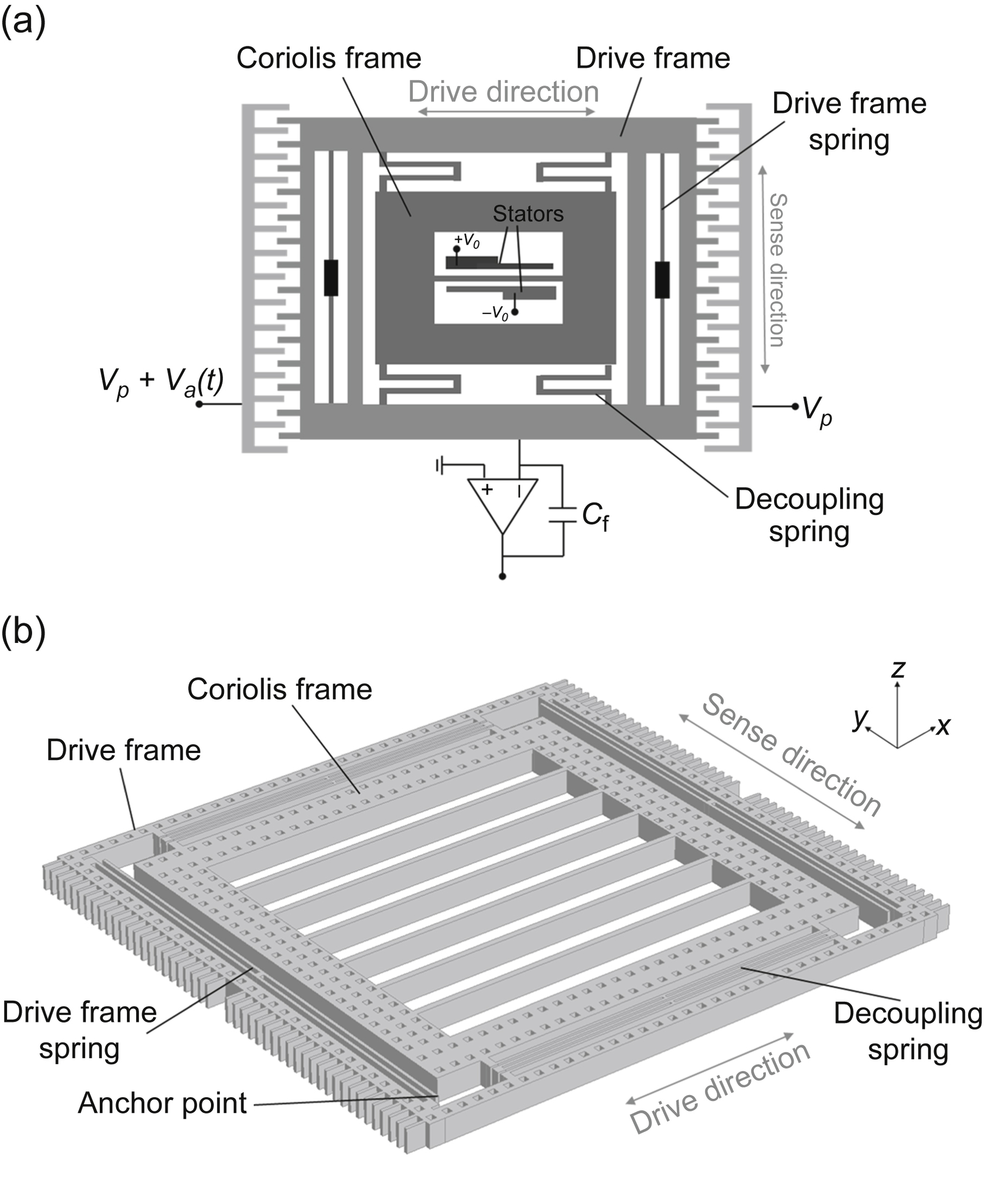
Figure 15.5 IIIustration of a single-mass gyroscope for sensing of angular rate along the z-axis. (a) Schematic top view with a simplified illustration of the voltages applied for driving and readout and (b) computer-aided design 3D view of the suspended mass showing the drive and Coriolis frame with the springs used to constrain the motion directions.
External accelerations in the y-direction can potentially disturb the measurement of the angular rate Ω as they can themselves determine a displacement of the Coriolis mass in the y-direction. To avoid this unwanted interference, the gyroscope can be designed in the dual-mass tuning fork configuration as reported in Fig. 15.6 (Geen et al., 2002; Acar et al., 2009; Raman et al., 2009; Dellea et al., 2015a,b,c). In this implementation, the two drive frames are mechanically coupled by a central spring and are excited in the antiphase mode. As a consequence, in presence of a Coriolis force, the Coriolis frames move in the opposite direction. Conversely, acceleration has a common mode effect that can be canceled out by adopting a differential readout. Further minimization of the signals caused by external vibrations can be obtained by filtering the acceleration signal, which (unless for very specific applications) typically occurs within a bandwidth <5–10 kHz, far from the gyroscope signal that instead occurs around the drive modulation frequency fD.
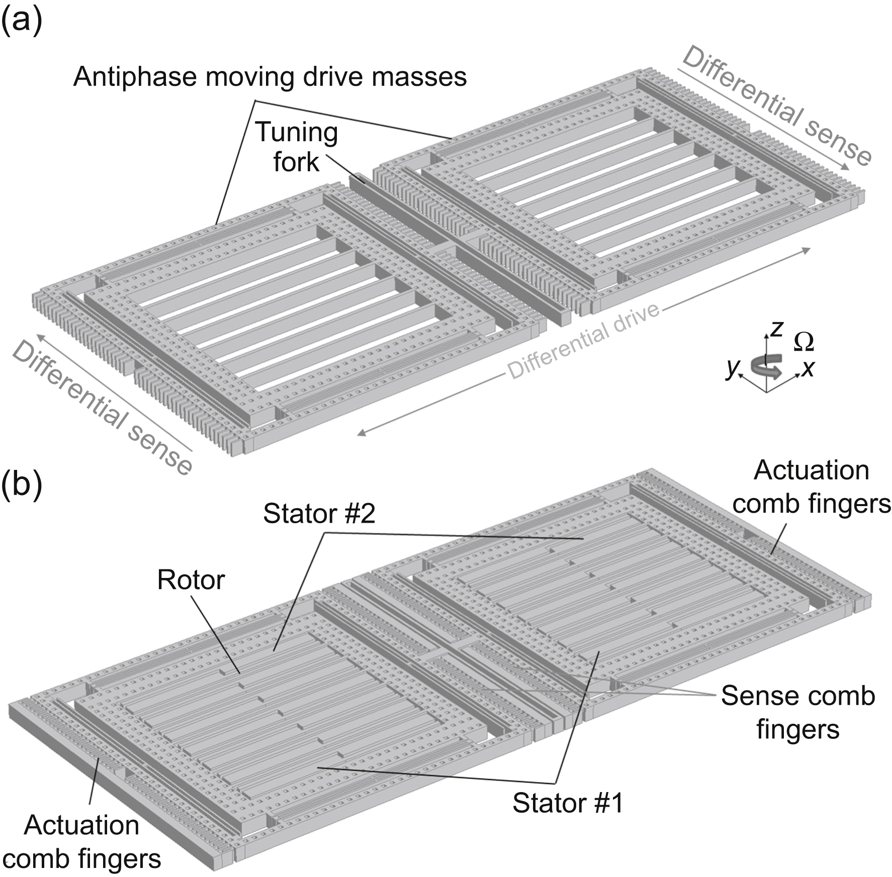
Figure 15.6 Illustration of a dual-mass tuning fork gyroscope. (a) View of the suspended frame with the tuning force, which is used to mechanically constrain the antiphase drive mode and (b) view of the full device with the comb fingers for the drive oscillation in the x-direction and the differential stators used for capacitive sensing of the Coriolis force.
For simplicity, the equations that follow will be initially derived for a single-mass gyroscope and finally combined by considering a differential capacitance readout such as that already described for the accelerometer.
15.3.2. Mechanical sensitivity
This section presents the main equations governing the operation of the MEMS gyroscope. In particular, we first consider the calculation of the velocity of the drive and Coriolis masses when suitable voltages are applied to the electrodes. The result is then used to calculate the Coriolis force and the obtained differential capacitance variation for a given angular rate.
As pointed out in the previous subsection, the drive frame and the Coriolis frame are kept in oscillation by applying appropriate voltages to the comb finger capacitances as shown in Fig. 15.5. This is accomplished by embedding the seismic masses as resonating elements inside a self-sustained oscillating circuit (Sharma et al., 2007; Prandi et al., 2011; Dellea et al., 2015b). Fig. 15.5 presents one version of a driving configuration; a DC voltage Vp is applied to both (right and left) the comb-finger stators and an AC voltage va(t) = va,max sin(2πfDt) is superimposed on only one of them; the seismic mass is considered to be kept at the ground voltage. Alternatively, the DC voltage can be applied to the suspended mass, with the AC voltage applied to one port only. In any of these two configurations, two electrostatic forces act on the drive and Coriolis frames:
where the capacitances CD,r and CD,l are the capacitances formed by the comb-finger stators on the right and the left sides of the drive frame, respectively. These capacitances can be written as:
In Eqs. (15.25a) and (15.25b), Ncell is the number of comb-finger cells, Lov is the overlap length of two fingers, x0 is the air gap in between them, x is the displacement of the drive and Coriolis frames along the x-axis, and h is the out-of-plane thickness of the fingers. Under the assumption that the AC voltage amplitude is much lower than the DC voltage, vD,max/4 ≪ Vp, the overall driving force acting on the two frames can be computed as:
One important aspect highlighted by Eq. (15.26) is that the net electrostatic force applied by means of comb finger capacitances is not a function of the displacement, unlike in parallel-plate capacitances. A force, which is thus extremely linear with the value of the applied AC voltage va(t), can be obtained even at large displacements. This is one of the main reasons why comb-finger actuation is preferred for the design of MEMS gyroscopes, where the sensitivity (as it will be shown shortly) is proportional to the maximum displacement of the Coriolis frame. In an alternative implementation known as push-pull actuation, the use of two drive electrodes and two sense electrodes cancels the second-order term and a linear result can be obtained without any small-signal approximations. Such implementations are, further, directly compatible with fully differential sensing stages (Minotti et al., 2017).
The motion of the drive and Coriolis frames along the x-direction is governed by the same motion equation presented in Section 15.2 for the accelerometer, which can be now written as:
mD and mCor are the mass values of the drive and Coriolis frames, respectively, and bD and kD are the damping factor and the elastic stiffness characterizing the movement of the frames along the x-axis (in particular, kD is related to the drive frame springs as represented in Fig. 15.5). Unlike accelerometers (which are operated at relatively high pressures (e.g.,≈20–100 mbar) and are characterized by a poor quality factor at least in consumer and automotive applications), MEMS gyroscopes are operated at low pressures (e.g., ≈0.1 – 1 mbar) to achieve high Q factors, in the order of several thousand to tens of thousands. This feature allows the exploitation of the peak in the transfer function (see Fig. 15.2) to amplify the effects of the Coriolis force. Indeed, the driving voltage va(t) is, because of the close-loop oscillation circuit, a sinusoidal signal at a frequency equal to the resonance frequency of the drive mode. Therefore, the displacement in the x-direction can be again written as a sine wave:
where
is the maximum value of the driving force FD(t).
The modulus of the Coriolis force, acting on the Coriolis frame along the y-axis in presence of an angular velocity Ω (expressed in degrees per second, dps), can be computed through Eq. (15.22) as:
where xD0 is the amplitude of the drive displacement. Such a displacement is usually kept controlled by means of amplitude gain control circuits.
Taking into account the fact that the drive frame is strongly constrained in the y-direction, the movement of the Coriolis frame along the y-axis—identified as the sense mode—is characterized by the following motion equation:
in which bS and kS are the damping factor and the elastic stiffness along the y-axis. In particular, the value of kS is related to the geometry of the decoupling springs as shown in Fig. 15.5. The corresponding transfer function between the displacement and the Coriolis force can be written as:
fS and QS being the resonance frequency and the quality factor of the sense mode, respectively. The displacement of the Coriolis frame can be computed by multiplying the Coriolis force by the modulus of Eq. (15.33), obtaining:
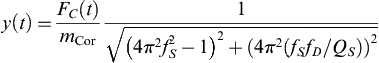 (15.34)
If we now consider the dual-mass tuning fork architecture shown in Fig. 15.6, Eq. (15.34) describes the opposite displacements of each of the two Coriolis frames depicted. Using a suitably designed array of differential parallel-plate capacitances, the capacitive variations of these two frames can be summed up to double the output signal while simultaneously filtering the possible interference of external accelerations, as described. By combining Eqs. (15.6) and (15.34), the mechanical sensitivity of the gyroscope, defined as the sense capacitance variation per angular velocity variation (F/dps), can be seen to be:
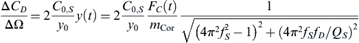 (15.35)
where C0,S and y0 are the capacitance and the air gap at rest between the parallel-plate stators and rotors forming each of the sensing capacitances.
It is now worth noting that the sensitivity depends to a considerable degree on the value and the relative difference of the resonance frequencies fD and fS of the drive and sense modes. Under the assumption of perfectly matched frequencies (known as mode matching, fD = fS), the sensitivity is maximized and can be written (in [F/dps]) as:
MEMS gyroscopes, especially when tailored for consumer applications, are in general designed with an fD and fS of around 20 kHz to minimize possible interference caused by vibration in the acoustic bandwidth (Dean et al., 2011).
Both the sensitivity and the signal bandwidth are a function of the frequency matching between the drive and the sense modes. Under the condition of matched frequencies, the bandwidth (in rad/s) of the gyroscope corresponds indeed to:
Eqs. (15.36) and (15.37) indicate a typical gain-bandwidth trade-off. For typical values of the frequency fS (20 kHz) and the quality factor QS (1000), the signal bandwidth obtained would be only 10 Hz. Typical applications—both in the consumer and the automotive markets (Neul et al., 2007) and even in the medical field (Della Santina, 2010)—require the measurement of angular rates on a larger bandwidth, around 50–100 Hz. Furthermore, because of process spread and temperature drift, keeping a gyroscope in matched conditions requires additional circuitry that is not compatible with low-power applications.
To solve this issue and to achieve a larger bandwidth, it is necessary to split the frequencies of the drive and the sense mode, by setting fS = fD + Δf; in this situation, the bandwidth of the gyroscope can be redefined as (Sharma et al., 2008; Langfelder et al., 2015):
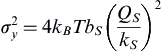
The mechanical sensitivity in the event of unmatched modes is significantly decreased because the quality factor of the sense mode is no longer fully exploited. In particular, for the range fS/2QS < Δf < fS, the mechanical sensitivity for the unmatched frequency condition can be expressed as:
which is the same expression as for the matched case but now with a larger bandwidth and a lower gain. Obtaining the same bandwidth in matched conditions would require a decrease in the value of the quality factor of the sense mode, obtainable only at the cost of an increased thermomechanical noise (see Eqs. (15.8) and (15.36) and consider that QS = ωS·mCor/bs). As a rule of thumb, the higher the required bandwidth is, the lower the mechanical sensitivity that can be obtained from a MEMS gyroscope. Fig. 15.7 reports a set of representative simulations, showing the normalized transfer function along the y-axis as a function of the frequency of the angular rate Ω for different mismatches between the drive and the sense modes.
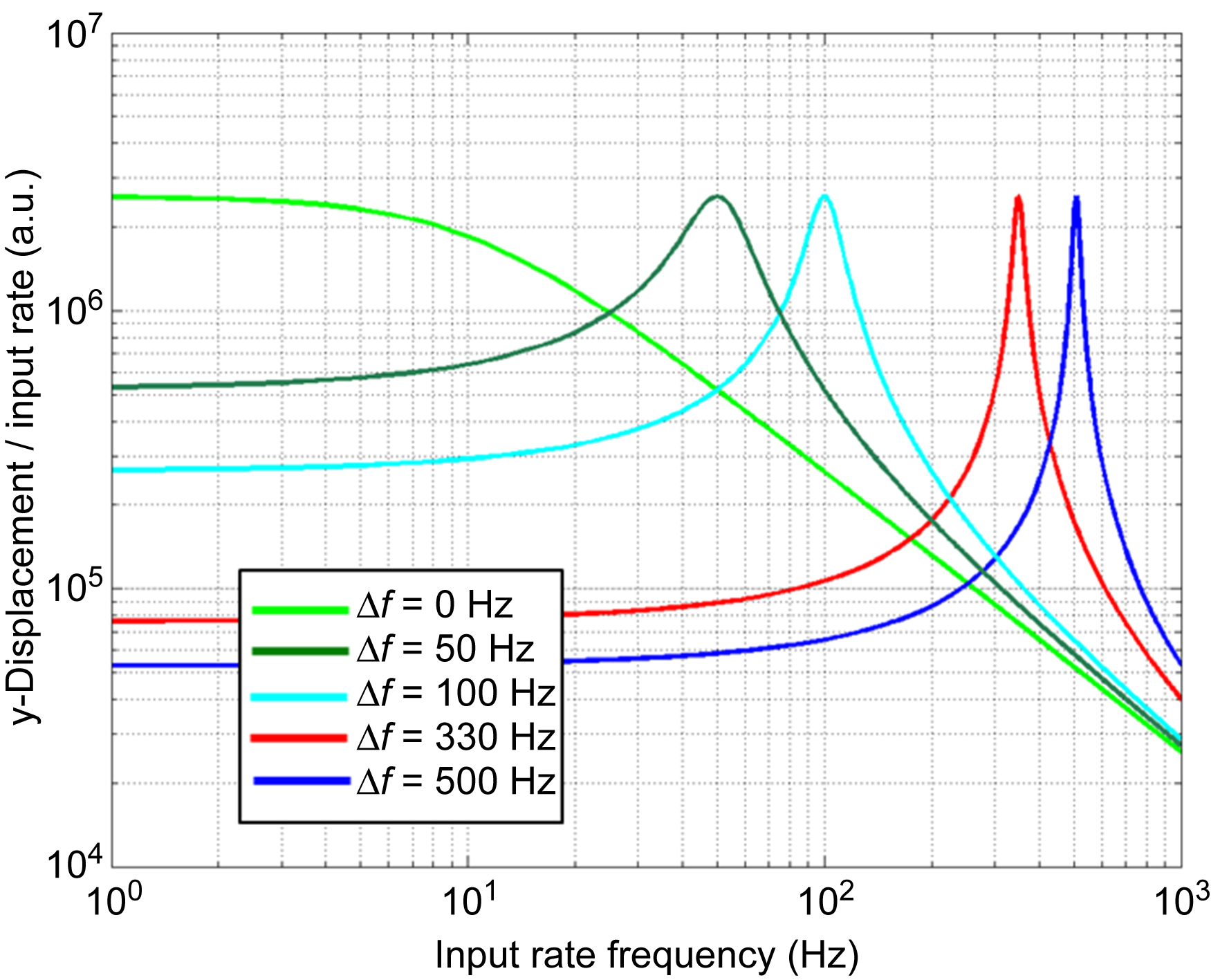
Figure 15.7 Transfer function of the Coriolis frame in the y-direction for the same angular rate as a function of the angular rate frequency. The different curves corresponds to different mismatches between the drive and sense modes. It can be observed that the larger the required bandwidth, the smaller the gain within the band.
Nowadays, 100% of consumer and automotive gyroscopes available on the market are based on mode-split operation (and not on mode-matched operation) for the reasons described above (Analog Devices, 2014; ST Microelectronics, 2014a,b; Maxim, 2014; ITmems, 2015; Invensense, 2013).
15.3.3. Intrinsic device noise
Even if the gyroscope operates at a pressures ∼1–2 orders of magnitude lower than the accelerometer, the intrinsic resolution of the device may be also in this situation affected by the thermomechanical noise associated with the Brownian motion of gas particles inside the packaging. This noise source causes random movement in all the different frames that constitute the gyroscope. Considering the gyroscope architecture described in the previous section, both the movements of the drive frame and the Coriolis frames along the x-axis and the movement of the Coriolis frame along the y-axis are affected by thermomechanical noise. Nevertheless, the dominant term is generally represented by the latter contribution, related to the Coriolis frames only. The drive frame thermomechanical noise has, to some extent, effects on the phase noise of the oscillator loop (Minotti et al., 2017). In particular, by using the definition of the noise power spectral density expressed in force (see Section 15.2), the noise power spectral density on the Coriolis frame, expressed in terms of displacement, can be computed as:
 (15.40)
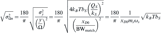
The native white noise contribution is therefore shaped by the transfer function of the sense mode, showing a peak around the resonance frequency fS, as represented in Fig. 15.8. Under the assumption of matched frequencies, the displacement noise power density (in [m2/Hz]) results:
 (15.41)
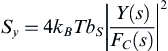
At this point, it is possible to evaluate the intrinsic noise density (i.e., the minimum detectable angular rate per unit bandwidth in dps/ ) of the device and the overall integrated root mean square (RMS) noise from the following formulas:
 (15.42)
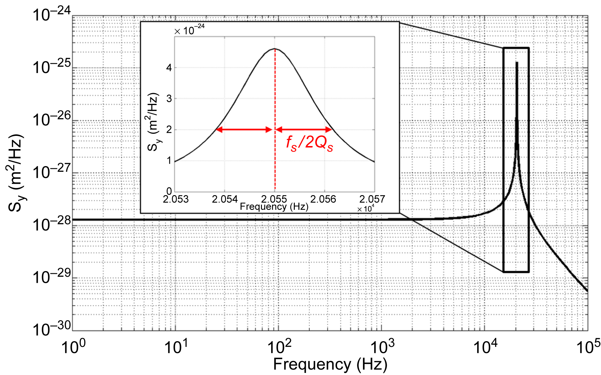
Figure 15.8 Example of noise power spectral density in terms of displacement, as shaped by the sense mode. The close-up shows a detail of the peak, highlighting the full width at half maximum equal to fSQS. After demodulation, signals can be filtered with a low-pass bandwidth equal to fS/2QS.
where BW is the minimum bandwidth between the device bandwidth and possible electronic filtering bandwidths. The reader can verify that in case of mode-split operation, the expression of the intrinsic noise density turns out to be identical. This should not be surprising, as thermomechanical noise represents force noise, and will be amplified like the Coriolis signal in the region around the low-pass filter used after demodulation.
The drawback of mode-split operation is, on the contrary, that electronic noise contributions will weigh more than for mode-matched frequencies, as—for the same intrinsic noise—the signal value is lower.
The considerations shown in this chapter can be easily extended to the design of gyroscopes for sensing the angular rate around the x and y axes (Prandi et al., 2011; Trusov et al., 2011; Dellea et al., 2015a,b,c). They can also be extended to gyroscopes with sensing means different from parallel plates, e.g., relying on the use of nano-electromechanical systems gages as proposed in Robert et al. (2009) and Dellea et al. (2015b).
15.3.4. References to resonant gyroscopes
Similarly to the case of accelerometers, resonant solutions have also been proposed for the gyroscopes. First idea had the purpose to augment the dynamic range and improve the resolution (see, e.g., Seshia et al., 2002b; Zotov et al., 2012). In this kind of device, the driving section is similar to that described for the capacitive gyroscopes, i.e., a suspended frame (or a pair of suspended frames) is kept in oscillation through a suitable driving circuit. The working principle for sensing is different from that of parallel-plate devices and is similar to that of resonant accelerometers (see Section 15.2.5); an angular rate results in a Coriolis acceleration, which determines a displacement that, in turn, causes a differential frequency shift of two resonating elements.
More interestingly, recent works have proposed the use of FM gyroscopes (Kline, 2013) to increase the stability of measurements, with the purpose of minimizing accumulated (integrated) errors for navigation applications, e.g., because of offset drifts generated by quadrature drifts (Weinberg and Kourepenis, 2006; Tatar et al., 2012) or by sensitivity drifts. In such devices, the operation is different from what described above, and the two modes (no longer a drive and a sense mode) are simultaneously kept in quadrature or Lissajous oscillation at controlled relative velocities (Kline et al., 2013; Izyumin et al., 2015). The effect of the Coriolis force is here to change the apparent frequency, seen from fixed electrodes, of both the modes, with a ratiometric scale factor.
Whatever the topology of FM gyroscopes is, the differential frequency shift is converted into a voltage difference that is thus proportional to the external angular rate.
15.4. Microelectromechanical systems magnetometer
There are many different methods by which a magnetic field can be sensed, depending on the intensity of the signal to be measured (Lenz, 2006). Magnetic fields can be as large as a few Tesla in MRI instrumentation; at the other end of the scale, the internal body activity manifests with minute magnetic field variations, as low as less than 1 nT. Therefore, given the large number of potential applications, there is an interest in developing miniaturized and low-power magnetic field sensors. For the applications of interest in this chapter, it is important to bear in mind that, typically, the Earth's magnetic field has values between 20 and 70 μT; to guarantee a precision in the measurement of the field direction of about 0.5–1 degrees, a resolution in the magnetic field measurement of about 0.1–0.5 μT per axis is required. Anisotropic magnetoresistance magnetometers cope with this requirement and also with relatively low-power operation (1 mW or fractions thereof). State-of-the-art magnetometers for consumer application IMUs are based on this principle (ST Microelectronics, 2014a,b) or on Hall effect or magnetic tunnel junctions. However, a complete IMU constructed in the same MEMS process would make devices very cheap, compact, and thus very attractive.
15.4.1. Working principle and mechanical sensitivity
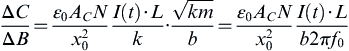
Among the possible approaches for the implementation of a magnetometer in MEMS technology, one of the most promising is based on the Lorentz force principle with capacitive readout (Emmerich and Schofthaler, 2000; Kyynäräinen et al., 2008; Thompson and Horsley, 2011aLangfelder et al., 2013). This is because it does not require the integration of magnetic materials in the realization process (see Fig. 15.9). A pair of longitudinal springs of length L holds a suspended shuttle that, with suitable stators, forms a set of differential capacitors C1 and C2, as described in the previous sections of this chapter. Suppose that a current I(t) is induced in both springs. In the presence of a component Bz of the magnetic field in the direction orthogonal to the plane of the figure, a force arises, which has a total intensity:
The force is orthogonal to the plane of both Bz and I(t), as depicted by the arrows in the figure. To give an initial idea of the intensity of this force, let us consider a spring length L = 1 mm (almost the maximum dimension reachable within a typical MEMS industrial package), a current I(t) = 1 mA (to cope with power dissipation, as will be clarified later), and the minimum field component to be detected Bz = 0.5 μT. It transpires that the force has an intensity of 0.5 pN for the pair of springs, which is more than 2 orders of magnitude lower than the inertial forces as seen in Section 15.2. As a means with which to amplify the displacement obtained from such a force, the device can be operated at resonance, with a displacement amplification given by the quality factor (see Fig. 15.2). Let us suppose that the current has the following expression: I(t) = I0 sin(2πf0t), where f0 is the device resonance frequency. If the device is packaged at low pressure (such as the gyroscope seen in the previous section), the displacement is amplified by the quality factor Q and is:
(the factor 2 at the denominator is justified by the fact that the force is distributed along the springs and is not concentrated on the shuttle). This modulation of the current also has the advantage that it modulates the signal at a large frequency, possibly out of the 1/f noise of the readout electronics.
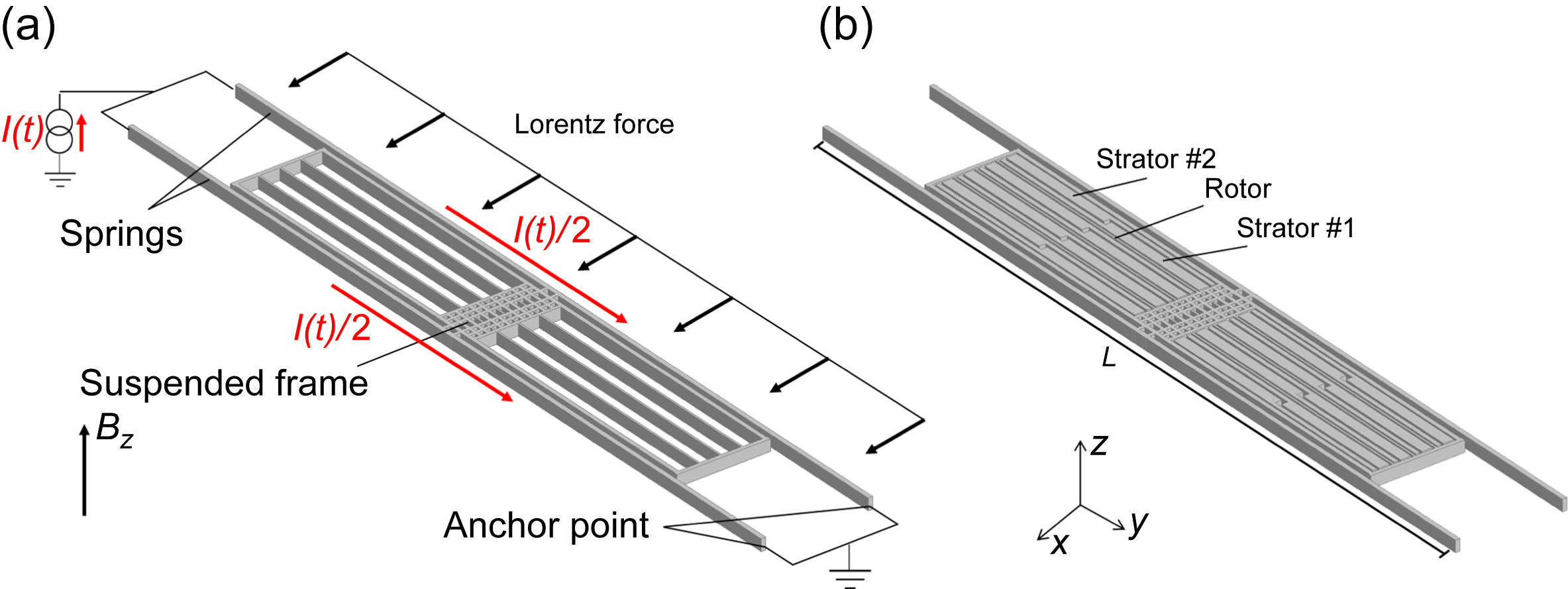
Figure 15.9 Illustration of a z-axis microelectromechanical systems magnetometer. (a) View of the suspended frame with a schematic of the working principle based on the Lorentz force arising in presence of a current I(t) and a magnetic field oriented in the z-direction and (b) view of the full device with the differential stators for capacitive sensing.
Consideration should be given here to the maximum Q that can be used; as the measurement bandwidth after the signal demodulation turns out to be equal to BW = f0/2Q to cope with typical required bandwidths for consumer and automotive applications (e.g., 50 Hz, see Table 15.1), the quality factor should not exceed a value that is 100 times lower than the resonance frequency.
By applying a differential capacitive readout technique, as seen in Section 15.2, the expression of the mechanical sensitivity (defined as the capacitance variation per unit of magnetic field change) can be derived, in the assumption of small displacements:
C0 being the value at rest of each of the differential capacitors used for the readout. If we assume that each capacitor is formed by N cells, each having an area AC, and if we write the expression of the quality factor in terms of the damping coefficient b, the following formula is obtained:
 (15.47)
It can be observed that, in principle, a low value of the resonance frequency f0 would be preferable. However, because of the tiny values of the magnetic force, it is generally better to design the device with a frequency out of the audio bandwidth (i.e., above ∼20 kHz) to avoid disturbances from amplified acoustic stimuli. As we have chosen f0, it is now possible to determine the maximum quality factor to cope with the said measurement bandwidth requirements:
The quality factor is determined by the damping coefficient b. This parameter depends mainly on the geometry adopted for the design of the sensing cells. It is the squeezed film effect that dominates in the pressure regime that can be obtained with typical industrial packages (Langfelder et al., 2011). As a consequence, damping is set by the squeezing of the air between the moving plates and the stators. Therefore, a careful choice of the gap between the parallel plates and their area has to be done to cope with the requirement of Eq. (15.48).
There are then practically only a few ways to increase, by means of design, the mechanical sensitivity of Lorentz force capacitive magnetometers: the maximization of the device length L (however, not convenient for area reasons); increasing the driving current I(t) (which is, however, limited by power dissipation constraints); and, more interestingly, the design of multiloops that make the current recirculate (Kyynäräinen et al., 2008; Minotti et al., 2015), and the recirculation of the same current across the three different axes, allowed by off-resonance operation (Langfelder and Tocchio, 2014; Laghi et al., 2015, Laghi et al., 2016). Great improvement can be obtained also if the process itself is improved by establishing narrower air gaps x0 between the parallel plates, which is common to any capacitive device.
The description given here for the z-axis magnetometer can be easily extended to the other axes—for instance, by using tilting structures (Thompson and Horsley, 2011b; Laghi et al., 2015, 2016) as previously mentioned regarding the accelerometer and the gyroscope.
Bahreyni and Shafai (2007) also suggest the use of resonant sensing for magnetometers (as described for accelerometers and gyroscopes in Sections 15.2.5 and 15.3.3). Innovative FM principles for magnetometers have been recently proposed also by Li et al. (2015).
15.4.2. Thermomechanical noise and intrinsic resolution
Let us now consider the effect of the thermomechanical noise power spectral density SF,n, as defined in Section 15.2. For sake of simplicity, it will be assumed that the signal will be later filtered by the electronics with a bandwidth equal to the signal bandwidth defined above, BW = f0/2Q (see Fig. 15.7). From Eq. (15.8), the noise power, reported in terms of displacement, can be expressed as:
Note that the random forces occur on the seismic mass and are not distributed to the springs. This explains the absence of a factor 2 at the denominator. The signal-to-noise ratio (SNR) can be then written as:
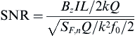 (15.50)
Finally, by putting the SNR equal to 1, the minimum measurable magnetic field can be derived as follows:
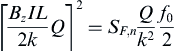 (15.51)
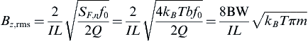 (15.52)
As an example, if we assume—as we have done so far—to have a driving current of 1 mA, a length of 1 mm, a resonance frequency of 20 kHz, a mass of 0.5 10−9 kg and a quality factor of 200, then a minimum measurable magnetic field of ∼1 μT is obtained, which show that MEMS magnetometers based on the Lorentz force can be used effectively in IMUs for the applications considered in this section.
Furthermore, by using a recirculation factor Nloop through multispiral loops and the recirculation of the same current through three devices, a further factor 3·Nloop lowers the minimum measurable signal. For example, with Nloop = 10 (Laghi et al., 2016), a resolution in the order of few hundred  can be obtained even at much lower currents (e.g., in the order of 100 μA only!). This definitely makes Lorentz force magnetometers attractive for future generation all-MEMS smart IMUs.
15.4.3. Effects of the readout electronics
It is worthwhile offering a brief discussion on the interdependence of the performances of the device and the readout electronics. This kind of discussion related to trade-offs between parameters could be done for every sensor, but it is particularly paradigmatic for magnetometers. Looking again at Eq. (15.52), it is evident that the more the current I is used to drive the device at resonance, the better the resolution. However, this implies a larger power dissipation by Joule effect in the springs, PMEMS = (I2·R), and in general a larger power dissipation by the circuit that generates such a current from a bias supply, PLorentz = I·VDD.
A similar consideration can be made for the electronic noise  , which we have not considered so far; as a rule of thumb, the more the power is dissipated in the electronics Peln, the better the noise performance. It can be concluded that, in the magnetometer design, the typical trade-off between resolution and power dissipation becomes a double trade-off, as summarized by the system below:
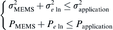 (15.53)
This is caused by the fact that, in Lorentz force-based magnetometers, there is an additional contribution to power dissipation inside the device, PLorentz—which is not present, for instance, in accelerometers. The conclusion that can be drawn from this is that the interdependence of the components of a MEMS magnetometer and its readout electronics is even greater than for other devices. Optimization must be achieved at system level and not by separately considering the two subsystems. A good analysis with experimental results on split of the power budget between device and circuit is given in Minotti et al. (2015).
15.5. Conclusion and future trends
The aim of this section is to outline the possible evolution of smart IMUs over the next 5–10 years. It has been shown that accelerometers, gyroscopes, and magnetometers can be designed using the same, relatively simple MEMS process and it is therefore expected that, in the very near future, (1–2 years) all-MEMS 9-DOF IMUs will be available. The reduced cost and dimensions of such IMUs will contribute to their widespread use in several fields of application. The next steps in the evolution of these devices can be identified at two different levels: hardware and software.
Innovation at the hardware level refers mainly to the development and integration of new devices, enabled by technological breakthroughs. As an example, another useful sensor that can be integrated into an all-MEMS IMU is the pressure sensor. This kind of sensor can be made using a suspended membrane (and not only a frame) and thus needs some modification to the technology (Zhang et al., 2011). Indeed, to obtain relatively large-sealed cavities made through a suspended membrane, it is necessary to change the process due to the fact that etching holes must be sealed after the release of movable parts. Sensing can be performed electrostatically through a bottom plate forming a capacitance, the value of which changes with the external pressure. Such a sensor would add a precise and independent measurement of the height of the IMU. This information could be exploited either for an initial calibration of the sensor position or for further online corrections of the estimated position. It could also give information on the height in those environments where the guide positioning systems signal is easily lost; an example is the identification of the height (or the floor) inside a building or a skyscraper. Ultralow-power MEMS pressure sensors with RMS pressure sensing noise in the order of 0.01 hParms are currently available on the market by several vendors (see, e.g., ST Microelectronics, 2016). Pressure sensors can be coupled to other miniaturized environmental sensors (humidity, temperature) to form micrometeorological stations.
From the electronics and software point of view, it becomes clear that the larger the number of parameters that the system is able to measure, the more complicated the overall combination of the useful information becomes. Electronics would not only read out and digitize the information from the single units but also process it to obtain more than the single, separate measurements (for instance, unwanted errors caused by an external acceleration on the measurements of other devices can be corrected online to augment precision because the acceleration is measured within the same IMU). It is thus foreseen that with the advent of such multifunction multiparameter sensors, the software requirements will become more complex for the sensor fusion calculations. For instance, there will likely be a need for microcontrollers rather than the usual ASICs.
15.5.1. Combination of inertial measurement units with proximity sensors
Once the displacement and the motion can be accurately measured, further smartness is added to the system if the surrounding environment can be recognized to some degree. Although infrared (IR) imaging sensors can be used to recover the distance of an object (Jin et al., 1998), their operation is typically limited to a low-light environment, unless high power consumption is spent in generating strong IR patterns. Furthermore, IR sensors are generally made with materials other than silicon and thus they are inherently expensive.
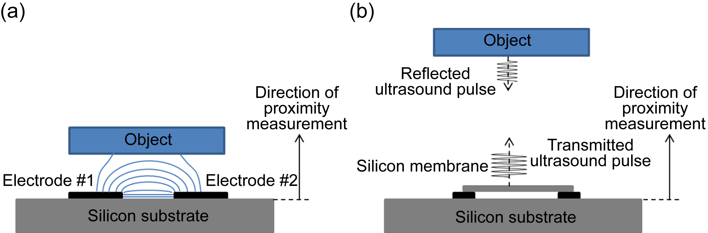
The development of capacitive proximity sensors can overcome this issue, as they can be made through micromachining technologies similar to those used for the devices previously described in this chapter (in particular they can leverage on technologies developed for microphones and pressure sensors). In its simplest form, a proximity sensor is made through a set of coplanar electrodes, which form a capacitance that is dominated by the fringe effects, as depicted in Fig. 15.10(a) (Chen and Luo, 1998). As a consequence, an object that moves in the volume surrounding the electrodes changes the distribution of the field lines and thus determines a capacitance change (Langfelder et al., 2012). The distance of the object moving above the electrodes can be measured if the object's material is known (a conductor or a dielectric will have different effects on the field lines; when considering a dielectric, the effect depends on its electrical permittivity, etc.). Typical measuring distances can range from a few μm to a few cm (Eun et al., 2008; Lo et al., 2012). As a consequence, this kind of proximity sensor is very useful in many industrial environments where space is very limited (microrobotics, machine automation, inspection tools, etc.).
Proximity sensors with a larger and material-independent measuring distance can be implemented because of the recent development of capacitive or piezoelectric micromachined ultrasound transducers. This kind of device can be obtained—in a similar manner to the pressure sensor—by building a sealed chamber with a membrane at the top and an electrode at the bottom (Saarilahti et al., 2002; Caspani et al., 2014). The bottom electrode is used both to excite the membrane electrostatically, to generate an ultrasound wave (typical frequencies between fractions to tens of MHz), and to sense the membrane capacitance variation when this is hit by the reflected wave. An array or a matrix (Jiang et al., 2016) of such ultrasound wave transceivers can be used to obtain a depth image of the surrounding environment with a range in the order of a meter. A smart sensor capable of precisely measuring its motion and simultaneously monitoring the surroundings can have an enormous number of applications in gesture recognition, fingerprint sensing, industrial automation, platform stabilization, medical equipment, and robotics.
The scenario presented in this concluding section can be completed or partially modified by new evolutions in the industrial technologies for the mass production of MEMS devices. The integration of piezoelectric or piezoresistive materials (Guedes et al., 2011), the integration of nanowires within a MEMS process (Whalter et al., 2012; Dellea et al., 2015c), the use of resonant sensors (Comi et al., 2010), and the use of device stacking through TSV (Fischer et al., 2011) are some examples of possible trends that can lead to further miniaturization and a higher degree of precision in sensing.
The era of Internet of things is approaching, and smart miniaturized MEMS motion sensors are a key element of this future breakthrough.
..................Content has been hidden....................
You can't read the all page of ebook, please click here login for view all page.