Software and Compiler Optimization for Microcontrollers, Embedded Processors, and DSPs
Michael C. Brogioli Polymathic Consulting, Austin, TX, United States
Abstract
Code optimization is a critical step in the development process as it directly impacts the ability of the system to do its intended job. Code that executes faster means more channels, more work performed, and competitive advantage. Code that executes in less memory enables more application features to fit into the cell phone. Code that executes with less overall power consumption increases battery life or reduces money spent on powering a base station. This chapter is intended to help programmers write the most efficient code possible, whether measured in processor cycles, memory, or power. It starts with an introduction to using toolchains, covers the importance of knowing about embedded architecture before optimization, then moves on to cover a wide range of optimization techniques. Techniques are presented which are valid on all programmable architectures—C-language optimization techniques and general loop transformations. Real-world examples are presented throughout.
Keywords
Optimization; Performance; Embedded Architecture; Compiler; Unrolling; Multisampling; Restrict; Intrinsic; Pragma; Power; Cache
1 Introduction
Optimization for embedded systems can involve several different factors at the software level, many of which directly reflect the underlying hardware. When optimizing embedded applications, the developer must be mindful of algorithmic requirements, supported arithmetic operations and data types, memory system layout, to name a few. In addition, developers must also be mindful of build tools and their optimizing capabilities, and just as important in certain cases, the inability of some tools to optimize. This chapter discusses selected features of modern embedded build tools, the use of data structures, data types, and how to best enable tools to extract the greatest optimization for a given application.
2 Development Tools Overview
It is important to understand the features of development tools as they provide many useful, time-saving opportunities. Modern compilers are increasingly performing better with embedded software, leading to a reduction in required development times. Linkers, debuggers, and other components of the toolchain have useful code-build and debugging features, but in this chapter we will only focus on compilers.
2.1 Compilers, Linkers, Loaders, and Assemblers
From the compiler perspective, there are two basic ways of compiling an application: traditional compilation or global (cross-file) compilation. In traditional compilation, each source file is compiled separately and then the generated objects are linked together. In global optimization, each C file is preprocessed and passed to the optimizer in the same file. This enables greater optimizations (interprocedural optimizations) to be made as the compiler has complete visibility of the program and doesn’t have to make conservative assumptions about the external functions and references. Global optimization does have some drawbacks, however. Programs compiled this way will take longer to compile and are harder to debug (as the compiler has taken away function boundaries and moved variables). In the event of a compiler bug, it will be more difficult to isolate and work around when built globally. Global or cross-file optimizations result in full visibility of all the functions, enabling much better optimizations for speed and size. The disadvantage is that since the optimizer can remove function boundaries and eliminate variables, the code becomes difficult to debug. Fig. 1 shows the compilation flow for each.

2.1.1 Basic Compiler Configuration
Before building for the first time, some basic configuration will be necessary. Perhaps the development tools come with project stationery and have basic options configured. If not, these items should be checked:
- • Target architecture: specifying the correct target architecture will allow the best code to be generated.
- • Endianness: perhaps the vendor sells silicon with only one endianness, perhaps the silicon can be configured. There will likely be a default option.
- • Memory model: different processors may have options for different memory model configurations.
- • Initial optimization level: it’s best to disable optimizations initially.
2.1.2 Enabling Optimizations
Optimizations may be disabled by default when no optimization level is specified and either new project stationery is created or code is built on the command line. Such code is designed for debugging only. With optimizations disabled, all variables are written and read back from the stack, enabling the programmer to modify the value of any variable via the debugger when stopped. This code is inefficient and should not be used in production code.
The levels of optimization available to the programmer will vary from vendor to vendor, but there are typically four levels (e.g., from zero to three), with three producing the most optimized code (Table 1). With optimizations turned off, debugging will be simpler because many debuggers have a hard time with optimized and out-of-order scheduled code, but the code will obviously be much slower (and larger). As the level of optimization increases, more and more compiler features will be activated, and compilation times will become longer.
Table 1
| Setting | Description |
|---|---|
| -O0 | Optimizations disabled. Outputs unoptimized assembly code |
| -O1 | Performs target independent high-level optimizations but no target-specific optimizations |
| -O2 | Target-independent and target-specific optimizations. Outputs nonlinear assembly code |
| -O3 | Target-independent and target-specific optimizations, with global register allocation. Outputs nonlinear assembly code. Recommended for speed-critical parts of the application |
Note that optimization levels are typically applied at the project, module, and function level using pragmas, allowing different functions to be compiled at different levels of optimization.
In addition, there will typically be an option to build for size, which can be specified at any optimization level. In practice, a few optimization levels are most often used: O3 (optimize fully for speed) and Os (optimize for size). In a typical application, critical code is optimized for speed and the bulk of the code may be optimized for size.
2.2 Peripheral Applications for Performance
Many development environments have a profiler, which enables the programmer to analyze where cycles are spent. These are valuable tools and should be used to find critical areas. The function profiler works in the IDE with the command line simulator.
3 Understanding the Embedded Target Architecture
Before writing code for an embedded processor, it’s important to assess the architecture itself and understand the resources and capabilities available. Modern embedded architectures have many features to maximize throughput. Table 2 provides some features that should be understood and some questions the programmer should ask.
Table 2
| Architectural Feature | Description |
|---|---|
| Instruction set architecture | Native multiply or multiply followed by add? Is saturation implicit or explicit? Which data types are supported—8, 16, 32, 40? Fractional and/or floating-point support? SIMD hardware? Does the compiler autovectorize, or are intrinsics required to access SIMD hardware? Domain-specific instructions (bit swapping, bit shift, Viterbi, video, etc.). Do these need to be accessed via intrinsics? |
| Register file | How many registers are there, how many register files comprise the total register set? What are they used for (integer, addressing, floating point)? Implication example: How many times can a loop be unrolled before performance decreases due to register pressure? How many live variables can be within a single scope at a time before spill code is generated? |
| Predication | Does the architecture support predicated execution? How many predicates does the architecture support? More predicates result in better control code performance. How efficient is the compiler at handling code generation for this feature? |
| Memory system | What kind of memory is available and what are the speed trade-offs between them? How many busses are there? How many read/write operations can be performed in parallel? Is there a data/instruction cache within the system? Are there small SRAM-based scratch pad buffers? Can bit-reversed addressing be performed? Is there support for circular buffers in the hardware? |
| Other | Hardware loops? Mode bits? If the compiler cannot determine the value of mode bits (saturating arithmetic, nonsaturating arithmetic) it may impact the ability to optimize code. |
The next few sections will cover aspects of embedded architectures and will address how to appropriately optimize an embedded application to take advantage of tools-based optimization as well as select architectural features.
4 Basic Optimization Goals and Practices
This section contains basic C optimization techniques that will benefit code written for all embedded processors. The central ideas are to ensure the compiler is leveraging all features of the architecture and to communicate to the compiler additional information about the program which is not communicated in C.
4.1 Data Types
It is important to learn about the sizes of the various types on the core before starting to write code. A compiler is required to support all required types but there may be performance implications and reasons to choose one type over another.
For example, a processor may not support a 32-bit multiplication. The use of a 32-bit data type in a multiply operation may cause the compiler to generate a sequence of multiple instructions, versus a single native multiply instruction. If 32-bit precision is not needed, it would be better to use 16-bit. Similarly, using a 64-bit type on a processor which does not natively support it will result in a similar construction of 64-bit arithmetic using 32-bit operations.
4.2 Intrinsics for Leveraging Embedded Processor Features
Intrinsic functions, or intrinsics for short, are a way to express either operations not possible or convenient to express in C or target-specific features (Table 3). Intrinsics in combination with custom data types can allow the use of nonstandard data sizes or types. They can also be used to get application-specific instructions (e.g., Viterbi or video instructions) which cannot be automatically generated from ANSI C by the compiler. They are used like function calls, but the compiler will replace them with the intended instruction or sequence of instructions. There is no calling overhead.
Table 3
| Example Intrinsic (C Language) | Generated Assembly Code |
|---|---|
| int d = L_add(a, b); | iadd d0, d1; |
Some examples of features accessible via intrinsics are saturating arithmetic, fractional data types, multiply accumulate, SIMD operations, and so forth. As a general rule, it is advisable to see what architectural features a given embedded processor supports at the ISA level and then review programmer manuals and build tools documentation to see how architectural features are accessed.
For example, an FIR filter can be rewritten to use intrinsics and therefore to specify processor operations natively (Fig. 2; FIR filter example). In this case, simply replacing the multiply and add operations with the intrinsic L_mac (for long multiply-accumulate) replaces two operations with one and adds the saturation function to ensure that digital signal processors (DSP) arithmetic is handled properly.

4.3 Calling Conventions and Application Binary Interfaces
Each processor or platform will have different calling conventions. Some will be stack-based, others register-based or a combination of both. Typically, default calling conventions can be overridden though, which is useful. The calling convention should be changed for functions unsuited to the default, like those with many arguments. In these cases, the calling conventions may be inefficient.
The advantages of changing a calling convention include the ability to pass more arguments in registers rather than on the stack. For example, on some embedded processors, custom calling conventions can be specified for any function through an application configuration file and pragmas. It’s a two-step process.
Custom calling conventions are defined by using the application configuration file (a file which is included in the compilation). Once defined a software developer can continue to develop their application as normal, however, if a developer wishes to use a custom-defined calling convention for certain function definitions, they must explicitly do so in the source code, often via #pragmas. For instance, if a custom calling convention named my_calling_convention is defined in the application configuration file, and the developer wishes to apply it to the test_calling_convention() function, the syntax may appear similar to that shown in Fig. 3:
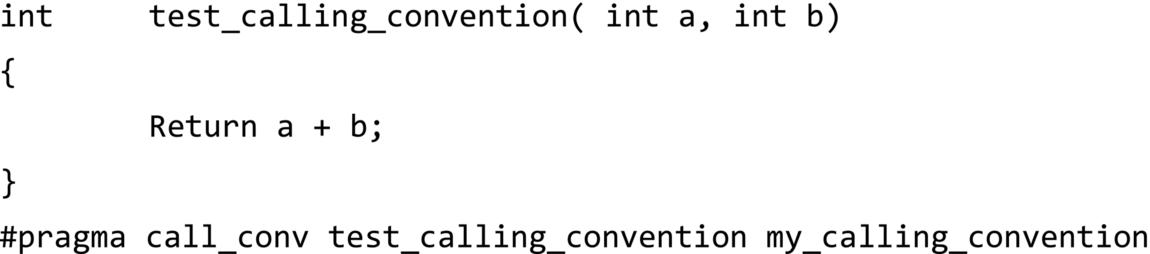
Developers should always refer to the documentation for their particular IDE and build environment, as well as application configuration files, to see the specific syntax used for a given toolchain and target architecture.
4.4 Memory Alignment
Some embedded processors, like DSPs, support loading of multiple data values across the busses as this is necessary to keep the arithmetic functional units busy. These moves are called multiple data moves (not to be confused with packedor vectormoves). They move adjacent values in memory to different registers. In addition, many compiler optimizations require these multiple register moves because there is so much data to move to keep all the functional units busy.
Typically, however, a compiler aligns variables in memory to their access width. For example, an array of short (16-bit) data is aligned to 16 bits. However, to leverage multiple data moves, the data must have a higher alignment. For example, to load two 16-bit values at once, the data must be aligned to 32 bits.
4.5 Pointers and Aliasing
When pointers are used in the same piece of code, make sure that they cannot point to the same memory location (alias). When the compiler knows the pointers do not alias, it can put accesses to memory pointed to by those pointers in parallel, greatly improving performance. Otherwise, the compiler must assume that the pointers could alias. This can be communicated to the compiler by one of two methods: using the restrict keyword or informing the compiler that no pointers alias anywherein the program (Fig. 4).

The restrict keyword is a type qualifier that can be applied to pointers, references, and arrays (Figs. 5 and 6). Its use represents a guarantee by the programmer that within the scope of the pointer declaration, the object pointed to can be accessed only by that pointer. A violation of this guarantee can produce undefined results.

4.6 Loops
Loops are one of the fundamental components of many embedded applications, especially in the DSP space where computation is often regular computation over blocks of code. Communicating information to the compiler about loops can be very important in achieving high performance within an application. Pragmas can be used to communicate information to the compiler about loop bounds to help loop optimization. If the loop minimum and maximum are known, for example, the compiler may be able to make more aggressive optimizations.
In the example in Fig. 7, a pragma is used to specify the loop count bounds to the compiler. In this syntax, the parameters are minimum, maximum, and multiple, as shown by the three numerical parameters as part of the loop_count pragma usage. If a nonzero minimum is specified, the compiler can avoid generation of costly zero-iteration checking code. The compiler can use the maximum and multiple parameters to know how many times to unroll the loop if possible.

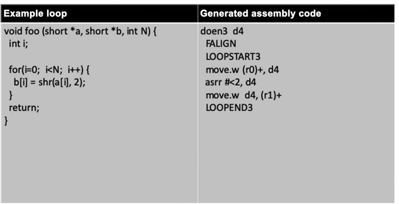
Reiterating the point that loop structures are a key component of all numerical processing applications and most embedded processing applications, hardware loops are another means of achieving performance within an application.
Hardware loops are mechanisms built into some embedded cores which allow zero- overhead (in most cases) looping by keeping the loop body in a buffer or by prefetching. Hardware loops are faster than normal software loops (decrement counter and branch) because they have less change-of-flow overhead. Hardware loops typically use loop registers that start with a count equal to the number of iterations of the loop, decrease by 1 each iteration (step size of 21), and finish when the loop counter is zero.
Compilers most often automatically generate hardware loops from C even if the loop counter or loop structure is complex. However, there will be certain criteria under which the compiler will be able to generate a hardware loop (which vary depending on compiler/architecture). In some cases the loop structure will prohibit generation, but if the programmer knows about this the source can be modified so the compiler can generate the loop using hardware loop functionality. The compiler may have a feature to tell the programmer if a hardware loop was not generated (compiler feedback). Alternatively, the programmer should check the generated code to ensure hardware loops are being generated for critical code. It is advisable to read the programmers manual for your target architecture and build tools to understand under what conditions the tools can, and cannot, generate hardware loops.
4.7 Advanced Tips and Tricks
The following are some additional tips and tricks that can be used to further increase the performance of compiled code. Note, however, that some of these concepts, like inlining of functions, may have adverse effects if used too aggressively—like impacts on code size.
Memory contention—When data is placed in memory, be aware of how the data is accessed. Depending on the memory type, if two buses issue data transactions in a region/bank/etc., they could conflict and cause a penalty. Data should be separated appropriately to avoid this contention. Scenarios that cause contention are device dependent because memory bank configuration and interleaving differs from device to device.
Unaligned memory accesses—In some embedded processors, devices support unaligned memory access. This is particularly useful for video applications. For example, a programmer might load four byte-values which are offset by one byte from the beginning of an area in memory. Typically, there is a performance penalty for doing this.
Cache accesses—In the caches, place data that is used together side by side in memory so that prefetching the caches is more likely to obtain the data before it is accessed. In addition, ensure that the loading of data for sequential iterations of the loop is in the same dimension as the cache prefetch.
Function Inlining—The compiler normally inlines small functions, but the programmer can force inlining of functions if for some reason it isn’t happening (e.g., if size optimization is activated). For small functions the save, restore, and parameter-passing overheads can be significant relative to the number of cycles of the function itself. Therefore inlining is beneficial. Also, inlining functions decreases the chance of an instruction cache miss because the function is sequential to the former caller function and is likely to be prefetched. Note that inlining functions increases the size of the code. On some processors, pragma inline forces every call of the function to be inlined.
5 General Loop Transformations
The optimization techniques described in this section are general in nature. They are critical to taking advantage of modern multi-ALU processors. A modern compiler will perform many of these optimizations, perhaps simultaneously. In addition, they can be applied on all platforms, at the C or assembly level. Therefore throughout this section, examples are presented in general terms, in C and in assembly.
5.1 Loop Unrolling
Loop unrolling is a technique whereby a loop body is duplicated one or more times. The loop count is then reduced by the same factor to compensate. Loop unrolling can enable other optimizations, such as multisampling, partial summation, and software pipelining.
Once a loop is unrolled, flexibility in coding is increased. For example, each copy of the original loop can be slightly changed. Different registers could be used in each copy. Moves can be done earlier and multiple register moves can be used. Fig. 8 shows an example of a for loop that has been unrolled by a factor of four. As can be seen on the right-hand side of the figure, the loop iterations have been reduced by a factor of four, while the amount of instruction level parallelism within the loop has increased, potentially enabling further optimization by the compiler.

5.2 Multisampling
Multisampling is a technique for maximizing the usage of multiple ALU execution units in parallel for the calculation of independent output values that have an overlap in input source data values. In a multisampling implementation, two or more output values are calculated in parallel by leveraging the commonality of input source data values in calculations. Unlike partial summation, multisampling is not susceptible to output value errors from intermediate calculation steps. Multisampling can be applied to any signal-processing calculation of the form:
where:

Using C pseudocode, the inner loop for the output value calculation can be written as:
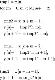
As can be seen above, the multisampled version works on Noutput samples at once. Transforming the kernel into a multisample version involves the following changes:
- • Changing the outer loop counters to reflect the multisampling by N.
- • Use of Nregisters for accumulation of the output data.
- • Unrolling the inner loop Ntimes to allow for common data elements in the calculation of the Nsamples to be shared.
- • Reducing the inner loop counter by a factor of Nto reflect the unrolling by N.
5.3 Partial Summation
Partial summation is an optimization technique whereby the computation for one output sum is divided into multiple smaller, or partial, sums. The partial sums are added together at the end of the algorithm. Partial summation allows more use of parallelism since some serial dependency is broken, allowing the operation to complete sooner.
Partial summation can be applied to any signal-processing calculation of the form:
![]() where:
where:
y[0] = x[0 + 0]h[0] + x[1 + 0]h[1] + x[2 + 0]h[2] + … + x[M + 0]h[M]
To perform a partial summation, each calculation is simply broken up into multiple sums. For example, for the first output sample, assuming M= 3:

Note the partial sums can be chosen as any part of the total calculation. In this example, the two sums are chosen to be the first + the second, and the third + the fourth calculations.
Important note: partial summation can cause saturation arithmetic errors. Saturation is not associative. For example, saturate(a*b) + c may not equal saturate (a*b + c). Care must be taken to ensure such differences do not affect program output.
The partial summed implementation works on Npartial sums at once. Transforming the kernel involves the following changes:
- • Use of Nregisters for accumulation of the Npartial sums.
- • Unrolling the inner loop will be necessary; the unrolling factor depends on the implementation, how values are reused, and how multiple register moves are used.
- • Changing the inner loop counter to reflect the unrolling.
5.4 Software Pipelining
Software pipelining is an optimization whereby a sequence of instructions is transformed into a pipeline of several copies of that sequence. The sequences then work in parallel to leverage more of the available parallelism of the architecture. The sequence of instructions can be duplicated as many times as needed, substituting a different set of registers for each sequence. Those sequences of instructions can then be interwoven.
For a given sequence of dependent operations:
A = operation();
B = operation(A);
C = operation(B);
Software pipelining gives (where operations on the same line can be parallelized):
A0 = operations();
B0 = operation(A); A1 = operation();
C0 = operation(B); B1 = operation(A1);
C1 = operation(B1);
5.5 Advanced Topics
For advanced reading in embedded optimization, and further case study analysis, please refer to Chapter 3. This section performs an in-depth analysis of an architectural breakdown of a wireless application, as well as relevant real-world embedded software optimizations to achieve desired performance results.
6 Code Size Optimization
In compiling a source code project for execution on a target architecture, it is often desirable for the resulting code size to be reduced as much as possible. The reasons for this pertain to both the amount of space in memory the code will occupy at program runtime and the potential reduction in the amount of instruction cache needed by the device. In reducing the code size of a given executable, a number of factors can be tweaked during the compilation process to accommodate this.
6.1 Compiler Flags and Flag Mining
Typically, users will first begin by configuring the compiler to build the program for size optimization, frequently using a compiler command line option like -Os, as available in the GNU GCC compiler version 4.5. When building for code size, it is not uncommon for the compiler to disable other optimizations that frequently result in improvements in the runtime performance of the code. Examples of these might be loop optimizations, such as loop unrolling or software pipelining, which typically are performed in an attempt to increase the runtime performance of the code at the cost of increases in the compiled code size. This is due to the fact that the compiler will insert additional code into the optimized loops, such as prolog and epilog code in the case of software pipelining or additional copies of the loop body in the case of loop unrolling.
In the event that users do not want to disable all optimization or build exclusively at optimization level -O0, with code size optimization enabled, users may also want to disable functionality like function inlining. This can be performed via either a compiler command line option or compiler pragma, depending on the system and functionality supported by the build tools. It is often the case that at higher levels of program optimization, specifically when optimizing for program runtime performance, compilers will attempt to inline copies of a function, whereby the body of the function code is inlined into the calling procedure, rather than the calling procedure being required to make a call into a callee procedure, resulting in a change of program flow and obvious system side effects. By specifying either as a command line option or via a customer compiler pragma, the user can prevent the tools from inadvertently inlining various functions which would result in an increase in the overall code size of the compiled application.
When a development team is building code for a production release, or in a use case scenario when debugging information is no longer needed in the executable, it may also be beneficial to strip out debugging information and symbol table information. In doing this, significant reductions in object file and executable file sizes can be achieved. Furthermore, in stripping out all label information, some level of IP protection may be afforded to the user in that consumers of the executable will have a difficult time reverse engineering the various functions being called within the program.
6.2 Target ISA for Size and Performance Trade-Offs
Various target architectures in the embedded space may afford additional degrees of freedom when trying to reduce the code size of the input application. Quite often it is advantageous for the system developer to take into consideration not only the algorithmic complexity and software architecture of their code but also the types of arithmetic required and how well those types of arithmetic and system requirements map to the underlying target architecture. For example, an application that requires heavy use of 32-bit arithmetic may run functionally on an architecture that is primarily tuned for 16-bit arithmetic; however, an architecture tuned for 32-bit arithmetic can provide a number of improvements in terms of both performance, code size, and perhaps power consumption.
Variable-length instruction encoding is one particular technology that a given target architecture may support, which can be effectively exploited by the build tools to reduce overall code size. In variable-length instruction coding schemes, certain instructions within the target processor’s ISA may have what is referred to as “premium encodings,” whereby those instructions most commonly used can be represented in a reduced binary footprint. One example of this might be a 32-bit embedded Power Architecture device, whereby frequently used instructions, like integer add, are also represented with a premium 16-bit encoding. When the source application is compiled for size optimization, the build tools will attempt to map as many instructions as possible to their premium encoding counterpart, in an attempt to reduce the overall footprint of the resulting executable.
Freescale Semiconductor supports this feature in the Power Architecture cores for embedded computing, as well as in their StarCore line of DSPs. Other embedded processor designs, such as those by ARM Limited and Texas Instruments’ DSP, have also employed variable encoding formats for premium instructions in an effort to curb the size of the resulting executable’s code footprint.
It should be mentioned than the reduced-footprint premium encoding of instructions in a variable-length encoding architecture often comes at the cost of reduced functionality. This is due to the reduction in the number of bits that are afforded in encoding the instruction, often reduced from 32 bits to 16 bits. An example of a nonpremium encoding instruction vs. a premium encoding instruction might be an integer arithmetic ADD instruction. On a nonpremium-encoded variant of the instruction, the source and destination operations of the ADD instruction may be any of the 32 general-purpose integer registers within the target architecture’s register file. In the case of a premium-encoded instruction, whereby only 16 bits of encoding space are afforded, the premium-encoded ADD instruction may only be permitted to use R0-R7 as source and destination registers, in an effort to reduce the number of bits used in the source and register destination encodings. Although it may not readily be apparent to the application programmer, this can result in subtle, albeit minor, performance degradations. These are often due to additional copy instructions that may be required to move source and destination operations around to adjacent instructions in the assembly schedule because of restrictions placed on the premium-encoded variants.
As evidence of the benefits and potential drawbacks of using variable-length encoding instruction set architectures as a vehicle for code size reduction, benchmarking of typical embedded codes when targeting Power Architecture devices has shown variable-length encoding (VLE)-enabled code to be approximately 30% smaller in code footprint size than standard Power Architecture code, while only exhibiting a 5% reduction in code performance. Resulting minor degradations in code performance are typical, due to limitations in functionality when using a reduced instruction encoding format of an instruction.
6.3 Caveat Emptor: Compiler Optimization Orthogonal to Code Size
When compiling code for a production release, developers often want to exploit as much compile-time optimization of their source code as possible in order to achieve the best performance possible. While building projects with -Os as an option will tune the code for optimal code size, it may also restrict the amount of optimization that is performed by the compiler due to such optimizations resulting in increased code size. As such, a user may want to keep an eye out for errant optimizations performed typically around loop nests and selectively disable them on a one-by-one use case rather than disable them for an entire project build. Most compilers support a list of pragmas that can be inserted to control compile-time behavior. Examples of such pragmas can be found in documentation accompanying the build tools for a processor.
Software pipelining is one optimization that can result in increased code size due to additional instructions that are inserted before and after the loop body of the transformed loop. When the compiler or assembly programmer software pipelines a loop, overlapping iterations of a given loop nest are scheduled concurrently with associated “set up” and “tear down” code inserted before and after the loop body. These additional instructions inserted in the set up and tear down, or prolog and epilog as they are often referred to in the compiler community, can result in increased instruction counts and code sizes. Typically, a compiler will offer a pragma such as “#pragma noswp” to disable software pipelining for a given loop nest, or given loops within a source code file. Users may want to utilize such a pragma on a loop-by-loop basis to reduce increases in code size associated with select loops that may not be performance-critical or on the dominant runtime paths of the application.
Loop unrolling is another fundamental compiler loop optimization that often increases the performance of loop nests at runtime. By unrolling a loop so that multiple iterations of the loop reside in the loop body, additional instruction-level parallelism is exposed for the compiler to schedule on the target processor; in addition, fewer branches with branch delay slots must be executed to cover the entire iteration space of the loop nest, potentially increasing the performance of the loop as well. Because multiple iterations of the loop are cloned and inserted into the loop body by the compiler, however, the body of the loop nest typically grows as a multiple of the unroll factor. Users wishing to maintain a modest code size may wish to selectively disable loop unrolling for certain loops within their code production, at the cost of compiled code runtime performance. By selecting those loop nests that may not be on the performance-critical path of the application, savings in code size can be achieved without impacting performance along the dominant runtime path of the application. Typically compilers will support pragmas to control loop unrolling-related behavior, such as the minimum number of iterations for which a loop will exist or various unroll factors to pass to the compiler. Examples of disabling loop unrolling via a pragma are often in the form “#pragma nounroll.” Please refer to your local compiler’s documentation for the correct syntax for this and related functionality.
7 Data Structures
Appropriate selection of data structures, before the design of kernels that compute over them, can have significant impact when dealing with high-performance embedded DSP codes. This is often especially true for target processors that support SIMD instruction sets and optimizing compiler technology, as was detailed previously. As an illustrative example, this section details the various trade-offs between using array-of-structure elements vs. structure-of-array elements for commonly used data structures as well as selection of data element sizes.
7.1 Arrays of Data Structures
As a data structure example, we’ll consider a set of six dimensional points that are stored within a given data structure as either an array of structures or a structure of arrays, as detailed in Fig. 9.

The array of structures, as depicted on the left-hand side of Fig. 9, details a structure that has six fields of floating-point type, each of which might be the three coordinates of the end points of a line in three-dimensional space. The structures are allocated as an array of SIZE elements. The structure of arrays, which is represented on the right-hand side, creates a single data structure that contains six arrays of floating-point data type, each of which is of SIZE elements. It should be noted that all the data structures above are functionally equivalent but have varying system side effects regarding memory system performance and optimization.
Looking at the array-of-structures example in the previous text, for a given loop nest that is known to access all the elements of a given struct element before moving onto the next element in the list, good locality of data will be exhibited. This will be because as cache lines of data are fetched from memory into the data cache lines, adjacent elements within the data structure will be fetched contiguously from memory and exhibit local reuse.
One downside when using the array-of-structures data structure, however, is that each individual memory reference in a loop that touches all the field elements of the data structure does not exhibit unit memory stride. For example, consider the illustrative loop in Fig. 10.
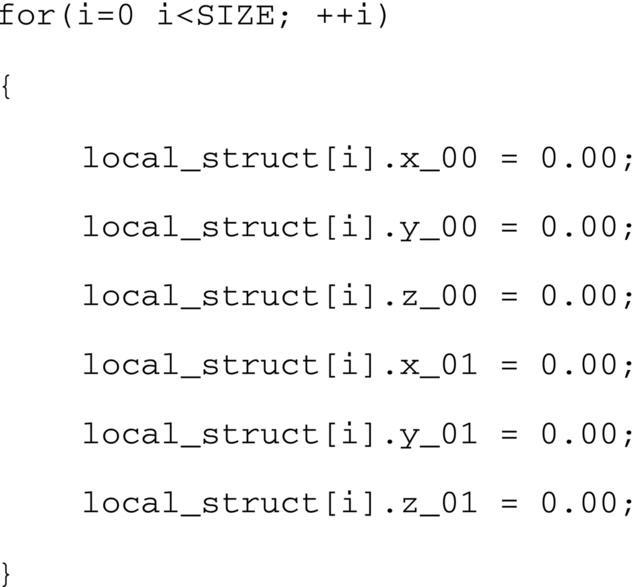
Each of the field accesses in the loop in Fig. 10 accesses different fields within an instance of the structure and does not exhibit unit stride memory access patterns which would be conducive to compiler-level autovectorization. In addition, any loop that traverses the list of structures and accesses only one or a few fields within a given structure instance will exhibit rather poor spatial locality of data within the cases, due to fetching cache lines from memory that contain data elements which will not be referenced within the loop nest.
In the next section, we see how migrating to an array-of-structures data format may work to the developer’s advantage.
7.2 Data Structures of Arrays
As seen above, using the array-of-structures format can result in suboptimal stride access patterns at runtime, thereby precluding some compile-time optimization. We can contrast the rather bleak use case depicted earlier by migrating the array-of- structures format to the structure-of-arrays format, as depicted in the loop nest in Fig. 11.

By employing the structure-of-arrays data structure, each field access within the loop nest exhibits unit stride memory references across loop iterations. This is much more conducive to autovectorization by the build tools in most cases. In addition, we still see good locality of data across the multiple array streams within the loop nest. It should also be noted that in contrast to the previous scenario, even if only one field is accessed by a given loop nest, locality within the cache is achieved due to subsequent elements within the array being prefetched for a given cache line load.
While the examples presented previously detail the importance of selecting the data structure that best suits the application developer’s needs, it is assumed that the developer or system architect will study the overall application hot spots in driving the selection of appropriate data structures for memory system performance. The result may not be a clear case of black and white, however, and a solution that employs multiple data structure formats may be advised. In these cases, developers may wish to use a hybrid-type approach that mixes and matches between structure-of-array and array-of-structure formats. Furthermore, for legacy code bases which, for various reasons, are tightly coupled to their internal data structures—an explanation of which falls outside the scope of this chapter—it may be worthwhile to runtime convert between the various formats as needed. While the computation required to convert from one format to another is nontrivial, there may be use cases where the conversion overhead is dramatically offset by the computational and memory system performance enhancements achieved once the conversion is performed.
7.3 SIMD-Based Optimization and Memory Alignment
In summary, data alignment details the way data is accessed within the computer’s memory system. The alignment of data within the memory system of an embedded target can have rippling effects on the performance of the code, as well as on the ability of development tools to optimize certain use cases. On many embedded systems, the underlying memory system does not support unaligned memory accesses, or such accesses are supported with a certain performance penalty. If the user does not take care in aligning data properly within the memory system layout, performance can be lost. Again, data alignment details the way data is accessed within the computer’s memory system. When a processor reads or writes to memory, it will often do this at the resolution of the computer’s word size, which might be 4 bytes on a 32-bit system. Data alignment is the process of putting data elements at offsets that are some multiple of the computer’s word size, so that various fields may be accessed efficiently. As such, it may be necessary for users to put padding into their data structures or for the tools to automatically pad data structures according to the underlying ABI and data type conventions when aligning data for a given processor target.
Alignment can have an impact on compiler and loop optimizations, like vectorization.
For instance, if the compiler is attempting to vectorize computation occurring over multiple arrays within a given loop body, it will need to know whether the data elements are aligned to make efficient use of packed SIMD move instructions, and to know whether certain iterations of the loop nest that execute over nonaligned data elements must be peeled off. If the compiler cannot determine whether the data elements are aligned, it may opt to not vectorize the loop at all, thereby leaving the loop body sequential in schedule. Clearly this is not the desired result for the best performing executable.
Alternatively, the compiler may decide to generate multiple versions of the loop nest with a runtime test to determine at loop execution time whether the data elements are aligned. In this case the benefits of a vectorized loop version are obtained; however, the cost of a dynamic test at runtime is incurred and the size of the executable will increase due to multiple versions of the loop nest being inserted by the compiler.
Users can often do multiple things to ensure that their data is aligned, for instance padding elements within their data structures and ensuring that various data fields lie on the appropriate word boundaries. Many compilers also support sets of pragmas to denote that a given element is aligned. Alternatively, users can put various asserts within their code to compute at runtime whether the data fields are aligned on a given boundary before a version of a loop executes.
7.3.1 Selecting Appropriate Data Types
It is important that application developers also select the appropriate data types for their performance-critical kernels in addition to the strategies of optimization. When the minimal acceptable data type is selected for computation, it may have several secondary effects that can be beneficial to the performance of the kernels. Consider, for example, a performance-critical kernel that can be implemented in either 32-bit integral computation or 16-bit integral computation due to the application programmer’s knowledge of the data range. If the application developer selects 16-bit computation using one of the built-in C/C11 language data types, like “short int,” then the following benefits may be gained at system runtime.
By selecting 16-bit over 32-bit data elements, more data elements can fit into a single data cache line. This allows fewer cache line fetches per unit of computation and should help alleviate the compute-to-memory bottleneck when fetching data elements. In addition, if the target architecture supports SIMD-style computation, it is highly likely that a given ALU within the processor can support multiple 16-bit computations in parallel vs. their 32-bit counterparts. For example, many commercially available DSP architectures support packed 16-bit SIMD operations per ALU, effectively doubling the computational throughput when using 16-bit data elements vs. 32-bit data elements. Given the packed nature of the data elements, whereby additional data elements are packed per cache line or can be placed in user-managed scratchpad memory, coupled with increased computational efficiency, it may also be possible to improve the power efficiency of the system due to the reduced number of data memory fetches required to fill cache lines.