Chapter 2
Auditory perception
In this chapter the mechanisms by which sound is perceived will be introduced. The human ear often modifies the sounds presented to it before they are presented to the brain, and the brain’s interpretation of what it receives from the ears will vary depending on the information contained in the nervous signals. An understanding of loudness perception is important when considering such factors as the perceived frequency balance of a reproduced signal, and an understanding of directional perception is relevant to the study of stereo recording techniques. Below, a number of aspects of the hearing process will be related to the practical world of sound recording and reproduction.
The hearing mechanism
Although this is not intended to be a lesson in physiology, it is necessary to investigate the basic components of the ear, and to look at how information about sound signals is communicated to the brain. Figure 2.1 shows a diagram of the ear mechanism, not anatomically accurate but showing the key mechanical components. The outer ear consists of the pinna (the visible skin and bone structure) and the auditory canal, and is terminated by the tympanic membrane or ‘ear drum’. The middle ear consists of a three-bone lever structure which connects the tympanic membrane to the inner ear via the oval window (another membrane). The inner ear is a fluid-filled bony spiral device known as the cochlea, down the centre of which runs a flexible membrane known as the basilar membrane. The cochlea is shown here as if ‘unwound’ into a straight chamber for the purposes of description. At the end of the basilar membrane, furthest from the middle ear, there is a small gap called the helicotrema which allows fluid to pass from the upper to the lower chamber. There are other components in the inner ear, but those noted above are the most significant.
The ear drum is caused to vibrate in sympathy with the air in the auditory canal when excited by a sound wave, and these vibrations are transferred via the bones of the middle ear to the inner ear, being subject to a multiplication of force of the order of 15:1 by the lever arrangement of the bones. The lever arrangement, coupled with the difference in area between the tympanic membrane and the oval window, helps to match the impedances of the outer and inner ears so as to ensure optimum transfer of energy. Vibrations are thus transferred to the fluid in the inner ear in which pressure waves are set up. The basilar membrane is not uniformly stiff along its length (it is narrow and stiff at the oval window end and wider and more flexible at the far end), and the fluid is relatively incompressible; thus a high-speed pressure wave travels through the fluid and a pressure difference is created across the basilar membrane.
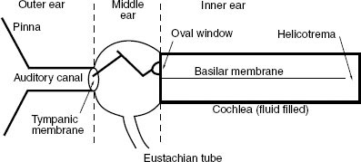
Figure 2.1 A simplified mechanical diagram of the ear
Frequency perception
The motion of the basilar membrane depends considerably on the frequency of the sound wave, there being a peak of motion which moves closer towards the oval window the higher the frequency (see Figure 2.2).
At low frequencies the membrane has been observed to move as a whole, with the maximum amplitude of motion at the far end, whilst at higher frequencies there arises a more well-defined peak. It is interesting to note that for every octave (i.e.: for every doubling in the frequency) the position of this peak of maximum vibration moves a similar length up the membrane, and this may explain the human preference for displaying frequency-related information on a logarithmic frequency scale, which represents increase in frequency by showing octaves as equal increments along a frequency axis.
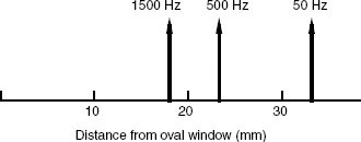
Figure 2.2 The position of maximum vibration on the basilar membrane moves towards the oval window as frequency increases
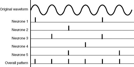
Figure 2.3 Although each neurone does not normally fire on every cycle of the causatory sound wave, the outputs of a combination of neurones firing on different cycles represent the period of the wave
Frequency information is transmitted to the brain in two principal ways. At low frequencies hair cells in the inner ear are stimulated by the vibrations of the basilar membrane, causing them to discharge small electrical impulses along the auditory nerve fibres to the brain. These impulses are found to be synchronous with the sound waveform, and thus the period of the signal can be measured by the brain. Not all nerve fibres are capable of discharging once per cycle of the sound waveform (in fact most have spontaneous firing rates of a maximum of 150 Hz with many being much lower than this). Thus at all but the lowest frequencies the period information is carried in a combination of nerve fibre outputs, with at least a few firing on every cycle (see Figure 2.3). There is evidence to suggest that nerve fibres may re-trigger faster if they are ‘kicked’ harder – that is, the louder the sound the more regularly they may be made to fire. Also, whilst some fibres will trigger with only a low level of stimulation, others will only fire at high sound levels.
The upper frequency limit at which nerve fibres appear to cease firing synchronously with the signal is around 4 kHz, and above this frequency the brain relies increasingly on an assessment of the position of maximum excitation of the membrane to decide on the pitch of the signal. There is clearly an overlap region in the middle-frequency range, from about 200 Hz upwards, over which the brain has both synchronous discharge information and ‘position’ information on which to base its measurement of frequency. It is interesting to note that one is much less able to determine the precise musical pitch of a note when its frequency is above the synchronous discharge limit of 4 kHz.
The frequency selectivity of the ear has been likened to a set of filters, and this concept is described in more detail in Fact File 2.1. It should be noted that there is an unusual effect whereby the perceived pitch of a note is related to the loudness of the sound, such that the pitch shifts slightly with increasing sound level. This is sometimes noticed as loud sounds decay, or when removing headphones, for example. The effect of ‘beats’ may also be noticed when two pure tones of very similar frequency are sounded together, resulting in a pattern of addition and cancellation as they come in and out of phase with each other. The so-called ‘beat frequency’ is the difference frequency between the two signals, such that signals at 200 Hz and 201 Hz would result in a cyclic modulation of the overall level, or beat, at 1 Hz. Combined signals slightly further apart in frequency result in a ‘roughness’ which disappears once the frequencies of the two signals are further than a critical band apart.
Fact file 2.1 Critical bandwidth
The basilar membrane appears to act as a rough mechanical spectrum analyser, providing a spectral analysis of the incoming sound to an accuracy of between one-fifth and one-third of an octave in the middle frequency range (depending on which research data is accepted). It acts rather like a bank of overlapping filters of a fixed bandwidth. This analysis accuracy is known as the critical bandwidth, that is the range of frequencies passed by each notional filter.
The critical band concept is important in understanding hearing because it helps to explain why some signals are ‘masked’ in the presence of others (see Fact File 2.3). Fletcher, working in the 1940s, suggested that only signals lying within the same critical band as the wanted signal would be capable of masking it, although other work on masking patterns seems to suggest that a signal may have a masking effect on frequencies well above its own.
With complex signals, such as noise or speech for example, the total loudness of the signal depends to some extent on the number of critical bands covered by a signal. It can be demonstrated by a simple experiment that the loudness of a constant power signal does not begin to increase until its bandwidth extends over more than the relevant critical bandwidth, which appears to support the previous claim. (A useful demonstration of this phenomenon is to be found on the Compact Disc entitled Auditory Demonstrations described at the end of this chapter.)
Although the critical band concept helps to explain the first level of frequency analysis in the hearing mechanism, it does not account for the fine frequency selectivity of the ear which is much more precise than one-third of an octave. One can detect changes in pitch of only a few hertz, and in order to understand this it is necessary to look at the ways in which the brain ‘sharpens’ the aural tuning curves. For this the reader is referred to Moore (2003), as detailed at the end of this chapter.
Loudness perception
The subjective quantity of ‘loudness’ is not directly related to the SPL of a sound signal (see ‘Sound power and sound pressure’, Chapter 1). The ear is not uniformly sensitive at all frequencies, and a set of curves has been devised which represents the so-called equal-loudness contours of hearing (see Fact File 2.2). This is partially due to the resonances of the outer ear which have a peak in the middle-frequency region, thus increasing the effective SPL at the ear drum over this range.
The unit of loudness is the phon. If a sound is at the threshold of hearing (just perceivable) it is said to have a loudness of 0 phons, whereas if a sound is at the threshold of pain it will probably have a loudness of around 140 phons. Thus the ear has a dynamic range of approximately 140 phons, representing a range of sound pressures with a ratio of around 10 million to one between the loudest and quietest sounds perceivable. As indicated in Fact File 1.4, the ‘A’-weighting curve is often used when measuring sound levels because it shapes the signal spectrum to represent more closely the subjective loudness of low-level signals. A noise level quoted in dBA is very similar to a loudness level in phons.
Fact file 2.2 Equal-loudness contours
Fletcher and Munson devised a set of curves to show the sensitivity of the ear at different frequencies across the audible range. They derived their results from tests on a large number of subjects who were asked to adjust the level of test tones until they appeared equally as loud as a reference tone with a frequency of 1 kHz. The test tones were spread across the audible spectrum. From these results could be drawn curves of average ‘equal loudness’, indicating the SPL required at each frequency for a sound to be perceived at a particular loudness level (see diagram).
Loudness is measured in phons, the zero phon curve being that curve which passes through 0 dB SPL at 1 kHz – in other words, the threshold of hearing curve. All points along the 0 phon curve will sound equally loud, although clearly a higher SPL is required at extremes of the spectrum than in the middle. The so-called Fletcher–Munson curves are not the only equal-loudness curves in existence – Robinson and Dadson, amongst others, have published revised curves based upon different test data. The shape of the curves depends considerably on the type of sound used in the test, since filtered noise produces slightly different results to sine tones.
It will be seen that the higher-level curves are flatter than the low-level curves, indicating that the ear’s frequency response changes with signal level. This is important when considering monitoring levels in sound recording (see text).

To give an idea of the loudnesses of some common sounds, the background noise of a recording studio might be expected to measure at around 20 phons, a low-level conversation perhaps at around 50 phons, a busy office at around 70 phons, shouted speech at around 90 phons, and a full symphony orchestra playing loudly at around 120 phons. These figures of course depend on the distance from the sound source, but are given as a guide.
The loudness of a sound depends to a great extent on its nature. Broad-band sounds tend to appear louder than narrow-band sounds, because they cover more critical bands (see Fact File 2.1), and distorted sounds appear psychologically to be louder than undistorted sounds, perhaps because one associates distortion with system overload. If two music signals are played at identical levels to a listener, one with severe distortion and the other without, the listener will judge the distorted signal to be louder.
A further factor of importance is that the threshold of hearing is raised at a particular frequency in the presence of another sound at a similar frequency. In other words, one sound may ‘mask’ another – a principle described in more detail in Fact File 2.3.
In order to give the impression of a doubling in perceived loudness, an increase of some 9–10 dB is required. Although 6 dB represents a doubling of the actual sound pressure, the hearing mechanism appears to require a greater increase than this for the signal to appear to be twice as loud. Another subjective unit, rarely used in practice, is that of the sone: 1 sone is arbitrarily aligned with 40 phons, and 2 sones is twice as loud as 1 sone, representing approximately 49 phons; 3 sones is three times as loud, and so on. Thus the sone is a true indication of the relative loudness of signals on a linear scale, and sone values may be added together to arrive at the total loudness of a signal in sones.
The ear is by no means a perfect transducer; in fact it introduces considerable distortions into sound signals due to its non-linearity. At high signal levels, especially for low-frequency sounds, the amount of harmonic and intermodulation distortion (see Appendix 1) produced by the ear can be high.
Practical implications of equal-loudness contours
The non-linear frequency response of the ear presents the sound engineer with a number of problems. Firstly, the perceived frequency balance of a recording will depend on how loudly it is replayed, and thus a balance made in the studio at one level may sound different when replayed in the home at another. In practice, if a recording is replayed at a much lower level than that at which it was balanced it will sound lacking in bass and extreme treble – it will sound thin and lacking warmth. Conversely, if a signal is replayed at a higher level than that at which it was balanced it will have an increased bass and treble response, sounding boomy and overbright.
A ‘loudness’ control is often provided on hi-fi amplifiers to boost low and high frequencies for low-level listening, but this should be switched out at higher levels. Rock-and-roll and heavy-metal music often sounds lacking in bass when replayed at moderate sound levels because it is usually balanced at extremely high levels in the studio.
Fact file 2.3 Masking
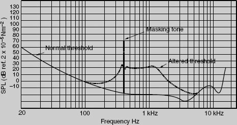
Most people have experienced the phenomenon of masking, although it is often considered to be so obvious that it does not need to be stated. As an example: it is necessary to raise your voice in order for someone to hear you if you are in noisy surroundings. The background noise has effectively raised the perception threshold so that a sound must be louder before it can be heard. If one looks at the masking effect of a pure tone, it will be seen that it raises the hearing threshold considerably for frequencies which are the same as or higher than its own (see diagram). Frequencies below the masking tone are less affected. The range of frequencies masked by a tone depends mostly on the area of the basilar membrane set into motion by the tone, and the pattern of motion of this membrane is more extended towards the HF end than towards the LF end. If the required signal produces more motion on the membrane than the masking tone produces at that point then it will be perceived.
The phenomenon of masking has many practical uses in audio engineering. It is used widely in noise reduction systems, since it allows the designer to assume that low-level noise which exists in the same frequency band as a high-level music signal will be effectively masked by the music signal. It is also used in digital audio data compression systems, since it allows the designer to use lower resolution in some frequency bands where the increased noise will be effectively masked by the wanted signal.
Some types of noise will sound louder than others, and hiss is usually found to be most prominent due to its considerable energy content at middle–high frequencies. Rumble and hum may be less noticeable because the ear is less sensitive at low frequencies, and a low-frequency noise which causes large deviations of the meters in a recording may not sound particularly loud in reality. This does not mean, of course, that rumble and hum are acceptable.
Recordings equalised to give a strong mid-frequency content often sound rather ‘harsh’, and listeners may complain of listening fatigue, since the ear is particularly sensitive in the range between about 1 and 5 kHz.
Spatial perception
Spatial perception principles are important when considering stereo sound reproduction (see Chapter 17) and when designing PA rigs for large auditoria, since an objective in both these cases is to give the illusion of directionality and spaciousness.
Sound source localisation
Most research into the mechanisms underlying directional sound perception conclude that there are two primary mechanisms at work, the importance of each depending on the nature of the sound signal and the conflicting environmental cues that may accompany discrete sources. These broad mechanisms involve the detection of timing or phase differences between the ears, and of amplitude or spectral differences between the ears. The majority of spatial perception is dependent on the listener having two ears, although certain monoaural cues have been shown to exist – in other words it is mainly the differences in signals received by the two ears that matter.
Time-based cues
A sound source located off the 0° (centre front) axis will give rise to a time difference between the signals arriving at the ears of the listener that is related to its angle of incidence, as shown in Figure 2.4. This rises to a maximum for sources at the side of the head, and enables the brain to localise sources in the direction of the earlier ear. The maximum time delay between the ears is of the order of 650 μs or 0.65 ms and is called the binaural delay. It is apparent that humans are capable of resolving direction down to a resolution of a few degrees by this method. There is no obvious way of distinguishing between front and rear sources or of detecting elevation by this method, but one way of resolving this confusion is by taking into account the effect of head movements. Front and rear sources at the same angle of offset from centre to one side, for example, will result in opposite changes in time of arrival for a given direction of head turning.
Time difference cues are particularly registered at the starts and ends of sounds (onsets and offsets) and seem to be primarily based on the low-frequency content of the sound signal. They are useful for monitoring the differences in onset and offset of the overall envelope of sound signals at higher frequencies.
Timing differences can be expressed as phase differences when considering sinusoidal signals. The ear is sensitive to interaural phase differences only at low frequencies and the sensitivity to phase begins to deteriorate above about 1 kHz. At low frequencies the hair cells in the inner ear fire regularly at specific points in the phase of the sound cycle, but at high frequencies this pattern becomes more random and not locked to any repeatable point in the cycle. Sound sources in the lateral plane give rise to phase differences between the ears that depend on their angle of offset from the 0°axis (centre front). Because the distance between the ears is constant, the phase difference will depend on the frequency and location of the source. (Some sources also show a small difference in the time delay between the ears at LF and HF.) Such a phase difference model of directional perception is only really relevant for continuous sine waves auditioned in anechoic environments, which are rarely heard except in laboratories. It also gives ambiguous information above about 700 Hz where the distance between the ears is equal to half a wavelength of the sound, because it is impossible to tell which ear is lagging and which is leading. Also there arise frequencies where the phase difference is zero. Phase differences can also be confusing in reflective environments where room modes and other effects of reflections may modify the phase cues present at the ears.
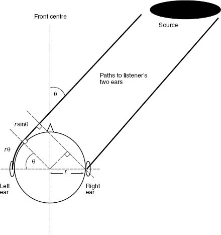
Figure 2.4 The interaural time difference (ITD) for a listener depends on the angle of incidence of the source, as this affects the additional distance that the sound wave has to travel to the more distant ear. In this model the ITD is given by r (θ+sin θ)/c (where c = 340 m/s, the speed of sound, and θ is in radians)
When two or more physically separated sources emit similar sounds the precedence effect is important in determining the apparent source direction, as explained in Fact file 2.4.
Fact file 2.4 The precedence effect
The precedence effect is important for understanding sound localisation when two or more sources are emitting essentially the same sound (e.g. a person speaking and a loudspeaker in a different place emitting an amplified version of their voice). It is primarily a feature of transient sounds rather than continuous sounds. In such an example both ears hear both the person and the loudspeaker. The brain tends to localise based on the interaural delay arising from the earliest arriving wavefront, the source appearing to come from a direction towards that of the earliest arriving signal (within limits).
This effect operates over delays between the sources that are somewhat greater than the interaural delay, of the order of a few milliseconds. Similar sound arriving within up to 50 ms of each other tend to be perceptually fused together, such that one is not perceived as an echo of the other. The time delay over which this fusing effect obtains depends on the source, with clicks tending to separate before complex sounds like music or speech. The timbre and spatial qualities of this ‘fused sound’, though, may be affected.
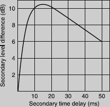
One form of precedence effect is sometimes referred to as the Haas Effect after the Dutch scientist who conducted some of the original experiments. It was originally identified in experiments designed to determine what would happen to the perception of speech in the presence of a single echo. Haas determined that the delayed ‘echo’ could be made substantially louder than the earlier sound before it was perceived to be equally loud, as shown in the approximation below. The effect depends considerably on the spatial separation of the two or more sources involved. This has important implications for recording techniques where time and intensity differences between channels are used either separately or combined to create spatial cues.
Amplitude and spectral cues
The head’s size makes it an appreciable barrier to sound at high frequencies but not at low frequencies. Furthermore, the unusual shape of the pinna (the visible part of the outer ear) gives rise to reflections and resonances that change the spectrum of the sound at the eardrum depending on the angle of incidence of a sound wave. Reflections off the shoulders and body also modify the spectrum to some extent. A final amplitude cue that may be relevant for spherical wave sources close to the head is the level difference due to the extra distance travelled between the ears by off-centre sources. For sources at most normal distances from the head this level difference is minimal, because the extra distance travelled is negligible compared with that already travelled.
The sum of all of these effects is a unique head-related transfer function or HRTF for every source position and angle of incidence, including different elevations and front–back positions. Some examples of HRTFs at different angles are shown in Figure 2.5. It will be seen that there are numerous spectral peaks and dips, particularly at high frequencies, and common features have been found that characterise certain source positions. This, therefore, is a unique form of directional encoding that the brain can learn. Typically, sources to the rear give rise to a reduced high-frequency response in both ears compared to those at the front, owing to the slightly forward-facing shape of the pinna. Sources to one side result in an increased high-frequency difference between the ears, owing to the shadowing effect of the head.
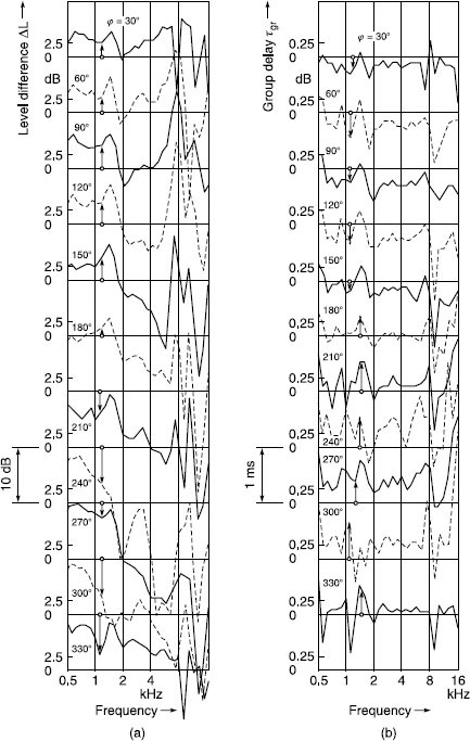
Figure 2.5 Monaural transfer functions of the left ear for several directions in the horizontal plane, relative to sound incident from the front; anechoic chamber, 2 m loudspeaker distance, impulse technique, 25 subjects, complex averaging (Blauert, 1997). (a) Level difference; (b) time difference. (Courtesy of MIT Press)
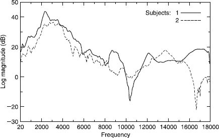
Figure 2.6 HRTFs of two subjects for a source at 0° azimuth and elevation. Note considerable HF differences. (Begault, 1991)
These HRTFs are superimposed on the natural spectra of the source themselves. It is therefore hard to understand how the brain might use the monoaural spectral characteristics of sounds to determine their positions as it would be difficult to separate the timbral characteristics of sources from those added by the HRTF. Monaural cues are likely to be more detectable with moving sources, because moving sources allow the brain to track changes in the spectral characteristics that should be independent of a source’s own spectrum. For lateralisation it is most likely to be differences in HRTFs between the ears that help the brain to localise sources, in conjunction with the associated interaural time delay. Monaural cues may be more relevant for localisation in the median plane where there are minimal differences between the ears.
There are remarkable differences in HRTFs between individuals, although common features can be found. Figure 2.6 shows just two HRTF curves measured by Begault for different subjects, illustrating the problem of generalisation in this respect.
The so-called concha resonance (that created by the main cavity in the centre of the pinna) is believed to be responsible for creating a sense of externalisation – in other words a sense that the sound emanates from outside the head rather than within. Sound-reproducing systems that disturb or distort this resonance, such as certain headphone types, tend to create in-the-head localisation as a result.
Effects of reflections
Reflections arising from sources in listening spaces affect spatial perception significantly, as discussed in Fact File 2.5. Reflections in the early time period after direct sound (up to 50–80 ms) typically have the effect of broadening or deepening the spatial attributes of a source. They are unlikely to be individually localisable. In the period up to about 20 ms they can cause severe timbral coloration if they are at high levels. After 80 ms they tend to contribute more to the sense of envelopment or spaciousness of the environment.
Fact file 2.5 Reflections affect spaciousness
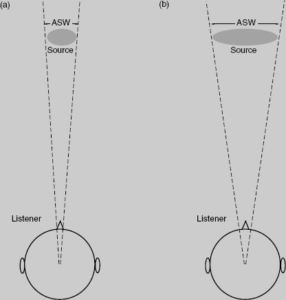
The subjective phenomenon of apparent or auditory source width (ASW) has been studied for a number of years, particularly by psychoacousticians interested in the acoustics of concert halls. ASW relates to the issue of how large a space a source appears to occupy from a sonic point of view (ignoring vision for the moment), as shown below. Individual source width should be distinguished from overall ‘sound stage width’ (in other words, the distance perceived between the left and right limits of a stereophonic scene).
Early reflected energy in a space (up to about 80 ms) appears to modify the ASW of a source by broadening it somewhat, depending on the magnitude and time delay of early reflections. Concert hall experiments seem to show that subjects prefer larger amounts of ASW, but it is not clear what is the optimum degree of ASW (presumably sources that appeared excessively large would be difficult to localise and unnatural).
Envelopment, spaciousness and sometimes ‘room impression’ are typically spatial features of a reverberant environment rather than individual sources, and are largely the result of late reflected sound (particularly lateral reflections after about 80 ms). Spaciousness is used most often to describe the sense of open space or ‘room’ in which the subject is located, usually as a result of some sound sources such as musical instruments playing in that space. It is also related to the sense of ‘externalisation’ perceived – in other words whether the sound appears to be outside the head rather than constrained to a region close to or inside it. Envelopment is a similar term and is used to describe the sense of immersivity and involvement in a (reverberant) soundfield, with that sound appearing to come from all around. It is regarded as a positive quality that is experienced in good concert halls.
Interaction between hearing and other senses
Some spatial cues are context dependent and may be strongly influenced by the information presented by other senses, particularly vision. Learned experience leads the brain to expect certain cues to imply certain spatial conditions, and if this is contradicted then confusion may arise. For example, it is unusual to experience the sound of a plane flying along beneath one, but the situation can occasionally arise when climbing mountains. Generally one expects planes to fly above, and most people will look up or duck when played loud binaural recordings of planes flying over, even if the spectral cues do not imply this direction.
It is normal to rely quite heavily on the visual sense for information about events within the visible field, and it is interesting to note that most people, when played binaural recordings (see Chapter 16) of sound scenes without accompanying visual information or any form of head tracking, localise the scene primarily behind them rather than in front. In fact obtaining front images from any binaural system using headphones is surprisingly difficult. This may be because one is used to using the hearing sense to localise things where they cannot be seen, and that if something cannot be seen it is likely to be behind. In the absence of the ability to move the head to resolve front–back conflicts the brain tends to assume a rear sound image. So-called ‘reversals’ in binaural audio systems are consequently very common.
Resolving conflicting cues
In environments where different cues conflict in respect of the implied location of sound sources, the hearing process appears to operate on a sort of majority decision logic basis. In other words it evaluates the available information and votes on the most likely situation, based on what it can determine. Auditory perception has been likened to a hypothesis generation and testing process, whereby likely scenarios are constructed from the available information and tested against subsequent experience (often over a very short time interval). Context-dependent cues and those from other senses are quite important here. Since there is a strong precedence effect favouring the first-arriving wavefront, the direct sound in a reflective environment (which arrives at the listener first) will tend to affect localisation most, while subsequent reflections may be considered less important. Head movements will also help to resolve some conflicts, as will visual cues. Reflections from the nearest surfaces, though, particularly the floor, can aid the localising process in a subtle way. Moving sources also tend to provide more information than stationary ones, allowing the brain to measure changes in the received information that may resolve some uncertainties.
Distance and depth perception
Apart from lateralisation of sound sources, the ability to perceive distance and depth of sound images is crucial to our subjective appreciation of sound quality. Distance is a term specifically related to how far away an individual source appears to be, whereas depth can describe the overall front–back distance of a scene and the sense of perspective created. Individual sources may also appear to have depth.
A number of factors appear to contribute to distance perception, depending on whether one is working in reflective or ‘dead’ environments. Considering for a moment the simple differences between a sound source close to a listener and the same source further away, the one further away will have the following differences:
• Quieter (extra distance travelled)
• Less high-frequency content (air absorbtion)
• More reverberant (in reflective environment)
• Less difference between time of direct sound and first-floor reflection
• Attenuated ground reflection
Numerous studies have shown that absolute distance perception, using the auditory sense alone, is very unreliable in non-reflective environments, although it is possible for listeners to be reasonably accurate in judging relative distances (since there is then a reference point with known distance against which other sources can be compared). In reflective environments, on the other hand, there is substantial additional information available to the brain. The ratio of direct to reverberant sound is directly related to source distance. The reverberation time and the early reflection timing tells the brain a lot about the size of the space and the distance to the surfaces, thereby giving it boundaries beyond which sources could not reasonably be expected to lie.
Naturalness in spatial hearing
The majority of spatial cues received in reproduced sound environments are similar to those received in natural environments, although their magnitudes and natures may be modified somewhat. There are, nonetheless, occasional phenomena that might be considered as specifically associated with reproduced sound, being rarely or never encountered in natural environments. The one that springs most readily to mind is the ‘out-of-phase’ phenomenon, in which two sound sources such as loudspeakers or headphones are oscillating exactly 180°out of phase with each other – usually the result of a polarity inversion somewhere in the signal chain. This creates an uncomfortable sensation with a strong but rather unnatural sense of spaciousness, and makes phantom sources hard to localise. The out-of-phase sensation never arises in natural listening and many people find it quite disorientating and uncomfortable. Its unfamiliarity makes it hard to identify for naïve listeners, whereas for expert audio engineers its sound is unmistakeable. Naïve listeners may even quite like the effect, and extreme phase effects have sometimes been used in low–end audio products to create a sense of extra stereo width.
Audio engineers also often refer to problems with spatial reproduction as being ‘phasy’ in quality. Usually this is a negative term that can imply abnormal phase differences between the channels, or an unnatural degree of phase difference that may be changing with time. Anomalies in signal processing or microphone technique can create such effects and they are unique to reproduced sound, so there is in effect no natural anchor or reference point against which to compare these experiences.
Recommended further reading
Blauert, J. (1997) Spatial Hearing, 2nd edition. Translated by J. S. Allen. MIT Press
Bregman, A. (1994) Auditory Scene Analysis: The Perceptual Organisation of Sound. MIT Press
Howard, D. and Angus, J. (2000) Acoustics and Psychoacoustics, 2nd edition. Focal Press
Moore, B. C. J. (2003) An Introduction to the Psychology of Hearing, 5th edition. Academic Press
Recommended listening
Auditory Demonstrations (Compact Disc). Philips Cat. No. 1126-061. Available from the Acoustical Society of America