
Chapter 1
Motivation for multivariate statistical process control
This first chapter outlines the basic principles of multivariate statistical process control. For the reader unfamiliar with statistical-based process monitoring, a brief revision of statistical process control (SPC) and its application to industrial process monitoring are provided in Section 1.1.
The required extension to MSPC to address data correlation is then motivated in Section 1.2. This section also highlights the need to extract relevant information from a large dimensional data space, that is the space in which the variation of recorded variables is described. The extracted information is described in a reduced dimensional data space that is a subspace of the original data space.
To help readers unfamiliar with MSPC technology, Section 1.3 offers a tutorial session, which includes a number of questions, small calculations/examples and projects to help familiarization with the subject and to enhance the learning outcomes. The answers to these questions can be found in this chapter. Project 2 to 4 require some self study and result in a detailed understanding on how to interpret SPC monitoring charts for detecting incipient fault conditions.
1.1 Summary of statistical process control
Statistical process control has been introduced into general manufacturing industry for monitoring process performance and product quality, and to observe the general process variation, exhibited in a few key process variables. Although this indicates that SPC is a process monitoring tool, the reference to control (in control engineering often referred to as describing and analyzing the feedback or feed-forward controller/process interaction), is associated with product or, more precisely, process improvement. In other words, the control objective here is to reduce process variation and to increase process reliability and product quality. One could argue that the controller function is performed by process operators or, if a more fundamental interaction with the process is required, a task force of experienced plant personnel together with plant managers. The next two subsections give a brief historical review of its development and outline the principles of SPC charts. The discussion of SPC in this section only represents a brief summary for the reader unfamiliar with this subject. A more in-depth and detailed treatment of SPC is available in references Burr (2005); Montgomery (2005); Oakland (2008); Smith (2003); Thompson and Koronacki (2002).
1.1.1 Roots and evolution of statistical process control
The principles of SPC as a system monitoring tool were laid out by Dr. Walter A. Shewhart during the later stages of his employment at the Inspection Engineering Department of the Western Electric Company between 1918 and 1924 and from 1925 until his retirement in 1956 at the Bell Telephone Laboratories. Shewhart summarized his early work on statistical control of industrial production processes in his book (Shewhart, 1931). He then extended this work which eventually led to the applications of SPC to the measurement processes of science and stressed the importance of operational definitions of basic quantities in science, industry and commerce (Shewhart, 1939). In particular, the latter book has had a profound impact upon statistical methods for research in behavioral, biological and physical sciences, as well as general engineering.
The second pillar of SPC can be attributed to Dr. Vilfredo Pareto, who first worked as a civil engineer after graduation in 1870. Pareto became a lecturer at the University of Florence, Italy from 1886, and from 1893 at the University of Lausanne, Switzerland. He postulated that many system failures are a result of relatively few causes. It is interesting to note that these pioneering contributions culminated in two different streams of SPC, where Shewhart's work can be seen as observing a system, whilst Pareto's work serves as a root cause analysis if the observed system behaves abnormally. Attributing the control aspect (root cause analysis) of SPC to the ‘Pareto Maxim’ implies that system improvement requires skilled personnel that are able to find and correct the causes of ‘Pareto glitches’, those being abnormal events that can be detected through the use of SPC charts (observing the system).
The work by Shewhart drew the attention of the physicists Dr. W. Edwards Deming and Dr. Raymond T. Birge. In support of the principles advocated by Shewart's early work, they published a landmark article on measurement errors in science in 1934 (Deming and Birge 1934). Predominantly Deming is credited, and to a lesser extend Shewhart, for introducing SPC as a tool to improved productivity in wartime production during World War II in the United States, although the often proclaimed success of the increased productivity during that time is contested, for example Thompson and Koronacki (2002, p5). Whilst the influence of SPC faded substantially after World War II in the United States, Deming became an ‘ambassador’ of Shewhart's SPC principles in Japan from the mid 1950s. Appointed by the United States Department of the Army, Deming taught engineers, managers including top management, and scholars in SPC and concepts of quality. The quality and reliability of Japanese products, such as cars and electronic devices, are predominantly attributed to the rigorous transfer of these SPC principles and the introduction of Taguchi methods, pioneered by Dr. Genichi Taguchi (Taguchi 1986), at all production levels including management.
SPC has been embedded as a cornerstone in a wider quality context, that emerged in the 1980s under the buzzword total quality management or TQM. This philosophy involves the entire organization, beginning from the supply chain management to the product life cycle. The key concept of ‘total quality’ was developed by the founding fathers of today's quality management, Dr. Armand V. Feigenbaum (Feigenbaum 1951), Mr. Philip B. Crosby (Crosby 1979), Dr. Kaoru Ishikawa (Ishikawa 1985) and Dr. Joseph M. Juran (Juran and Godfrey 2000). The application of SPC nowadays includes concepts such as Six Sigma, which involves DMAIC (Define, Measure, Analyze, Improve and Control), QFD (Quality Function Deployment) and FMEA (Failure Modes and Effect Analysis) (Brussee, 2004). A comprehensive timeline for the development and application of quality methods is presented in Section 1.2 in Montgomery (2005).
1.1.2 Principles of statistical process control
The key measurements discretely taken from manufacturing processes do not generally describe constant values that are equal to the required and predefined set points. In fact, if the process operates at a steady state condition, then these set points remain constant over time. The recorded variables associated with product quality are of a stochastic nature and describe a random variation around their set point values in an ideal case.
1.1.2.1 Mean and variance of a random variable
The notion of an ideal case implies that the expectation of a set of discrete samples for a particular key variable converges to the desired set point. The expectation, or ‘average’, of a key variable, further referred to as a process variable z, is described as follows
1.1 ![]()
where E{ · } is the expectation operator. The ‘average’ is the mean value, or mean, of z, ![]() , which is given by
, which is given by
In the above equation, the index k represents time and denotes the order when the specific sample (quality measurement) was taken. Equation (1.2) shows that ![]() as K → ∞. For large values of K, however, we can assume that
as K → ∞. For large values of K, however, we can assume that ![]() and small K values may lead to significant differences between
and small K values may lead to significant differences between ![]() and
and ![]() . The latter situation, that is, small sample sizes, may present difficulties if no set point is given for a specific process variable and the average therefore needs to be estimated. A detailed discussion of this is given in Section 6.4.
. The latter situation, that is, small sample sizes, may present difficulties if no set point is given for a specific process variable and the average therefore needs to be estimated. A detailed discussion of this is given in Section 6.4.
So far, the mean of a process variable is assumed to be equal to a predefined set point ![]() and the recorded samples describe a stochastic variation around this set point. The following data model can therefore be assumed to describe the samples
and the recorded samples describe a stochastic variation around this set point. The following data model can therefore be assumed to describe the samples
1.3 ![]()
The stochastic variation is described by the stochastic variable z0 and can be captured by an upper bound and a lower bound or the control limits which can be estimated from a reference set of the process variable. Besides a constant mean, the second main assumption for SPC charts is a constant variance of the process variable
where σ is defined as the standard deviation and σ2 as the variance of the stochastic process variable. This parameter is a measure for the spread or the variability that a recorded process variable exhibits. It is important to note that the control limits depend on the variance of the recorded process variable.
For a sample size K the estimate ![]() may accordingly depart from
may accordingly depart from ![]() and Equation (1.4) is, therefore, an estimate of the variance σ2,
and Equation (1.4) is, therefore, an estimate of the variance σ2, ![]() . It is also important to note that the denominator K − 1 is required in (1.4) instead of K since one degree of freedom has been used for determining the estimate of the mean value,
. It is also important to note that the denominator K − 1 is required in (1.4) instead of K since one degree of freedom has been used for determining the estimate of the mean value, ![]() .
.
1.1.2.2 Probability density function of a random variable
Besides a constant mean and variance of the process variable, the third main assumption for SPC charts is that the recorded variable follows a Gaussian distribution. The distribution function of a random variable is discussed later and depends on the probability density function or PDF. Equation (1.5) shows the PDF of the Gaussian distribution
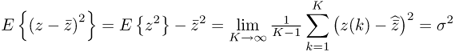
Figure 1.1 shows the Gaussian density function for ![]() = 0 and various values of σ. In this figure the abscissa refers to values of z and the ordinate represents the ‘likelihood of occurrence’ of a specific value of z. It follows from Figure 1.1 that the smaller σ the narrower the Gaussian density function becomes and vice versa. In other words, the variation of the variable depends on the parameter σ. It should also be noted that the value of ± σ represents the point of inflection on the curve f(z) and the maximum of this function is at z =
= 0 and various values of σ. In this figure the abscissa refers to values of z and the ordinate represents the ‘likelihood of occurrence’ of a specific value of z. It follows from Figure 1.1 that the smaller σ the narrower the Gaussian density function becomes and vice versa. In other words, the variation of the variable depends on the parameter σ. It should also be noted that the value of ± σ represents the point of inflection on the curve f(z) and the maximum of this function is at z = ![]() , i.e. this value has the highest chance of occurring. Traditionally, a stochastic variable that follows a Gaussian distribution is abbreviated by
, i.e. this value has the highest chance of occurring. Traditionally, a stochastic variable that follows a Gaussian distribution is abbreviated by ![]() .
.
Figure 1.1 Gaussian density function for ![]() = 0 and σ = 0.25, σ = 1.0 and σ = 2.0.
= 0 and σ = 0.25, σ = 1.0 and σ = 2.0.
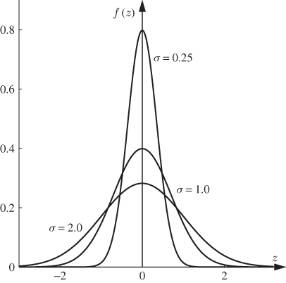
By closer inspection of (1.4) and Figure 1.1, it follows that the variation (spread) of the variables covers the entire range of real numbers, from minus to plus infinity, since likelihood values for very small or large values are nonzero. However, the likelihood of large absolute values is very small indeed, which implies that most values for the recorded variable are centered in a narrow band around ![]() . This is graphically illustrated in Figure 1.2, which depicts a total of 20 samples and the probability density function f(z) describing the likelihood of occurrence for each sample. This figure shows that large departures from
. This is graphically illustrated in Figure 1.2, which depicts a total of 20 samples and the probability density function f(z) describing the likelihood of occurrence for each sample. This figure shows that large departures from ![]() can occur, e.g. samples 1, 3 and 10, but that most of samples center closely around
can occur, e.g. samples 1, 3 and 10, but that most of samples center closely around ![]() .
.
Figure 1.2 Random Gaussian distributed samples of mean ![]() and variance σ.
and variance σ.
1.1.2.3 Cumulative distribution function of a random variable
We could therefore conclude that the probability of z values that are far away from ![]() is small. In other words, we can simplify the task of monitoring the process variable by defining an upper and a lower boundary that includes the vast majority of possible cases and excludes those cases that have relatively small likelihood of occurrence. Knowing that the integral over the entire range of the probability density function is equal to 1.0, the probability is therefore a measure for defining these upper and lower boundaries. For the symmetric Gaussian probability density function, the probability within the range bounded by
is small. In other words, we can simplify the task of monitoring the process variable by defining an upper and a lower boundary that includes the vast majority of possible cases and excludes those cases that have relatively small likelihood of occurrence. Knowing that the integral over the entire range of the probability density function is equal to 1.0, the probability is therefore a measure for defining these upper and lower boundaries. For the symmetric Gaussian probability density function, the probability within the range bounded by ![]() and
and ![]() is defined as
is defined as
Here, ![]() and
and ![]() defines the size of this range that is centered at
defines the size of this range that is centered at ![]() , 0 ≤ F( · ) ≤ 1.0, F( · ) is the cumulative distribution function and α is the significance, that is the percentage, α · 100%, of samples that could fall outside the range between the upper and lower boundary but still belong to the probability density function f( · ). Given that the Gaussian PDF is symmetric, the chance that a sample has an ‘extreme’ value falling in the left or the right tail end is
, 0 ≤ F( · ) ≤ 1.0, F( · ) is the cumulative distribution function and α is the significance, that is the percentage, α · 100%, of samples that could fall outside the range between the upper and lower boundary but still belong to the probability density function f( · ). Given that the Gaussian PDF is symmetric, the chance that a sample has an ‘extreme’ value falling in the left or the right tail end is ![]() . The general definition of the Gaussian cumulative distribution function F(a, b) is as follows
. The general definition of the Gaussian cumulative distribution function F(a, b) is as follows
1.7 
where Pr{ · } is defined as the probability that z assumes values that are within the interval [a, b].
1.1.2.4 Shewhart charts and categorization of process behavior
Assuming that ![]() = 0 and σ = 1.0, the probability of 1 − α = 0.95 and 1 − α = 0.99 yield ranges between
= 0 and σ = 1.0, the probability of 1 − α = 0.95 and 1 − α = 0.99 yield ranges between ![]() and
and ![]() . This implies that 5% and 1% of recorded values can be outside this ‘normal’ range by chance alone, respectively. Figure 1.3 gives an example of this for
. This implies that 5% and 1% of recorded values can be outside this ‘normal’ range by chance alone, respectively. Figure 1.3 gives an example of this for ![]() = 10.0, σ = 1.0 and α = 0.01. This implies that the upper boundary or upper control limit, UCL, and the lower boundary or lower control limit, LCL, are equal to 10 + 2.58 = 12.58 and 10 − 2.58 = 7.42, respectively. Figure 1.3 includes a total of 100 samples taken from a Gaussian distribution and highlights that one sample, sample number 90, is outside the ‘normal’ region. Out of 100 recorded samples, this is 1% and in line with the way the control limits, that is, the upper and lower control limits, have been determined. Loosely speaking, 1% of samples might violate the control limits by chance alone.
= 10.0, σ = 1.0 and α = 0.01. This implies that the upper boundary or upper control limit, UCL, and the lower boundary or lower control limit, LCL, are equal to 10 + 2.58 = 12.58 and 10 − 2.58 = 7.42, respectively. Figure 1.3 includes a total of 100 samples taken from a Gaussian distribution and highlights that one sample, sample number 90, is outside the ‘normal’ region. Out of 100 recorded samples, this is 1% and in line with the way the control limits, that is, the upper and lower control limits, have been determined. Loosely speaking, 1% of samples might violate the control limits by chance alone.
Figure 1.3 Schematic diagram showing statistical process control chart.
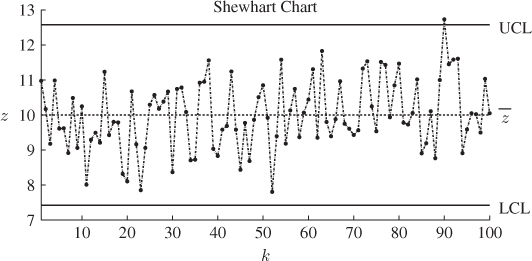
From the point of an interpretation of the SPC chart in Figure 1.3, which is defined as a Shewhart chart, samples that fall between the UCL and the LCL categorize in-statistical-control behavior of the recorded process variable and samples that are outside this region are indicative of an out-of-statistical-control situation. As discussed above, however, it is possible that α · 100% of samples fall outside the control limits by chance alone. This is further elaborated in Subsection 1.1.3.
1.1.2.5 Trends in mean and variance of random variables
Statistically, for quality related considerations a process is out-of-statistical-control if at least one of the following six conditions is met:
The process that is said to be an in-statistical-control process if none of the above hypotheses are accepted. Such a process is often referred to as a stable process or a process that does not present a trend. Conversely, if at least one of the above conditions is met the process has a trend that manifest itself in changes of the mean and/or variance of the recorded random variable. This, in turn, requires a detailed and careful inspection in order to identify the root cause of this trend. In essence, the assumption of a stable process is that a recorded quality variable follows a Gaussian distribution that has a constant mean and variance over time.
1.1.2.6 Control limits vs. specification limits
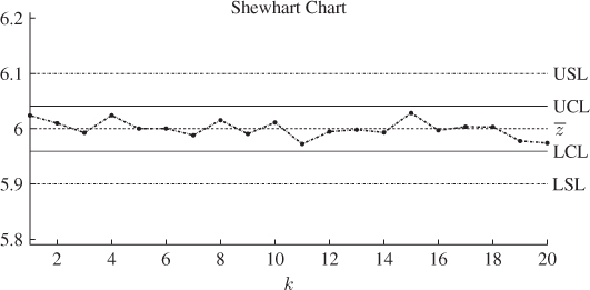
Up until now, the discussion has focussed on the process itself. This discussion has led to the definition of the control limits for process variables that follow a Gaussian distribution function and have a constant mean value, or set point, and variances have been obtained. More precisely, rejecting all of the above six hypotheses implies that the process is in-statistical control or stable and does not describe any trend. For SPC, it is of fundamental importance that the control limits of the key process variable(s) are inside the specification limits for the product. The specification limits are production tolerances that are defined by the customer and must be met. If the upper and lower control limits are within the range defined by the upper and lower specification limits, or USL and LSL, a stable process produces items that are, by default, within the specification limits. Figure 1.4 shows the relationship between the specification limits, the control limits and the set point of a process variable z for which 20 consecutively recorded samples are available.
Figure 1.4 Upper and lower specification limit as well as upper and lower control limits and set point value for key variable z.
1.1.2.7 Types of processes
Using the definition of the specification and control limits, a process can be categorized into a total of four distinct types:
The process shown in Figure 1.4 is an ideal process, where the product is almost always within the specification limits. An ideal process is therefore a stable process, since the mean and variance of the key product variable z is time invariant. A promising process is a stable process but the control limits are outside the region defined by the specification limits. The promising process has the potential to produce a significant amount of off-spec product.
The treacherous process is an unstable process, as the mean and/or variance of z varies over time. For this process, the absolute difference of the control limits is assumed to be smaller than the absolute difference of the specification limits. Similar to a promising process, a treacherous process has the potential to produce significant off-spec product although this is based on a change in mean/variance of z. Finally, a turbulent process is an unstable process for which the absolute difference of the control limits is larger than the absolute difference of the specification limits. The turbulent process therefore often produces off-spec products.
1.1.2.8 Determination of control limits
It is common practice for SPC applications to determine the control limits zα as a product of σ, for example the range for the UCL and LCL are ± σ, ± 2σ etc. Typical are three sigma and six sigma regions. It is interesting to note that the control limits that represent three sigma capture 99.73% of cases, which appears to describe almost all possible cases. It is important to note, however, that if a product is composed of say 50 items each of which has been produced within a UCL and LCL that correspond to ± 3σ, then the probability that any of the products does not conform to the required specification is 1 − (1 − α)50 = 1 − 0.997350 = 1 − 0.8736 = 0.1664, which is 16.64% and not 0.27%. It is common practice in such circumstances to determine UCL and LCL with respect to ± 6σ, that is α = 1 − 0.999999998, for which the same calculation yields that the probability that one product does not conform to the required specification reduces to 0.01 parts per million.
1.1.2.9 Common cause vs. special cause variation
Another concept that is of importance is the analysis as to what is causing the variation of the process variable z. Whilst this can be regarded as a process specific entity, two distinct sources have been proposed to describe this variation, the common cause variation and the special cause variation. The properties of common cause variation are that it arises all the time and is relatively small in magnitude. As an example for common cause variation, consider two screws that are produced in the same shift and selected randomly. These screws are not identical although the differences in thread thickness, screw length etc. are relatively small. The differences in these key variables must not be a result of an assignable cause. Moreover, the variation in thread length and total screw length must be process specific and cannot be removed. An attempt to reduce common cause variation is often regarded as tampering and may, in fact, lead to an increase in the variance of the recorded process variable(s). A special cause variation on the other hand, has an assignable cause, e.g. the introduction of disturbances, a process fault, a grade change or a transition between two operating regions. This variation is usually rare but may be relatively large in magnitude.
1.1.2.10 Advances in designing statistical process control charts
Finally, improvements for Shewhart type charts have been proposed in the research literature for detecting incipient shifts in ![]() (that is
(that is ![]() departs from
departs from ![]() over time), and for dealing with cases where the samples distribution function slightly departs from a Gaussian distribution. This has led to the introduction of cumulative sum or CUSUM charts (Hawkins 1993; Hawkins and Olwell 1998) and exponentially weighted moving average or EWMA charts (Hunter 1986; Lucas and Saccucci 1990).
over time), and for dealing with cases where the samples distribution function slightly departs from a Gaussian distribution. This has led to the introduction of cumulative sum or CUSUM charts (Hawkins 1993; Hawkins and Olwell 1998) and exponentially weighted moving average or EWMA charts (Hunter 1986; Lucas and Saccucci 1990).
Next, Subsection 1.1.3 summarizes the statistically important concept of hypothesis testing. This test is fundamental in evaluating the current state of the process, that is, to determine whether the process is in-statistical-control or out-of-statistical-control. Moreover, the next subsection also introduces errors associated with this test.
1.1.3 Hypothesis testing, Type I and II errors
To motivate the underlying meaning of a hypothesis test in an SPC context, Figure 1.5 describes the two scenarios introduced in the preceding discussion. The upper graph in this figure exemplifies an in-statistical-control situation, since:
- the recorded samples, z(k), are drawn from the distribution described by f0(z); and
- the confidence region, describing the range limited by the upper and lower control limits of this process, has been calculated by Equation 1.6 using f0(z)
Hence, the recorded samples fall inside the confidence region with a significance of α. The following statement provides a formal description of this situation.
![]()
In mathematical statistics, such a statement is defined as a hypothesis and referred to as H0. As Figure 1.5 highlights, a hypothesis is a statement concerning the probability distribution of a random variable and therefore its population parameters, for example the mean and variance of the Gaussian distribution function. Consequently, the hypothesis H0 that the process is in-statistical-control can be tested by determining whether newly recorded samples fall within the confidence region. If this is the case then the hypothesis that the process is in-statistical-control is accepted.
Figure 1.5 Graphical illustration of Type I and II errors in an SPC context.
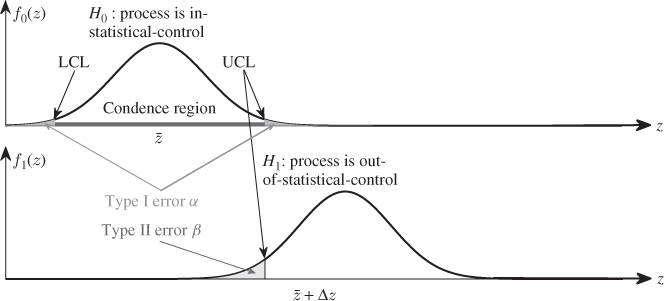
For any hypothesis testing problem, the hypothesis H0 is defined as the null hypothesis and is accompanied by the alternative hypothesis H1. In relation to the terminology introduced in the previous subsection, the statement governing the alternative hypothesis is as follows:
![]()
The lower plot in Figure 1.5 gives an example of an out-of-statistical-control situation by a shift in the mean of z from ![]() to
to ![]() + Δz. In general, if the null hypothesis is rejected the alternative hypothesis is accepted. This implies that if the newly recorded samples fall outside the confidence region the alternative hypothesis is accepted and the process is out-of-statistical-control. It should be noted that detecting an out-of-statistical-control situation, which is indicative of abnormal process behavior, is important but does not address the subsequent question as to what has caused this behavior. In fact, the diagnosis of anomalous process behavior can be considerably more challenging than detecting this event (Jackson 2003).
+ Δz. In general, if the null hypothesis is rejected the alternative hypothesis is accepted. This implies that if the newly recorded samples fall outside the confidence region the alternative hypothesis is accepted and the process is out-of-statistical-control. It should be noted that detecting an out-of-statistical-control situation, which is indicative of abnormal process behavior, is important but does not address the subsequent question as to what has caused this behavior. In fact, the diagnosis of anomalous process behavior can be considerably more challenging than detecting this event (Jackson 2003).
It is also important to note that testing the null hypothesis relies on probabilistic information, as it is related to the significance level α. If we assume a significance of 0.01, 99% of samples are expected to fall within the confidence region on average. In other words, this test is prone to mistakes and a sample that has an extreme value is likely to be outside the confidence region although it still follows f0(z). According to the discussion above, however, this sample must be considered to be associated with the alternative hypothesis H1. This error is referred to as a Type I error.
Figure 1.5 also illustrates a second error that is associated with the hypothesis testing. Defining the PDF corresponding to the shift in mean of z from ![]() to
to ![]() + Δz by f1( · ), it is possible that a recorded sample belongs to f1( · ) but its value is with the control limits. This scenario is defined as a Type II error.
+ Δz by f1( · ), it is possible that a recorded sample belongs to f1( · ) but its value is with the control limits. This scenario is defined as a Type II error.
The Type I error is equal to the significance level α for determining the upper and lower control limits. However, the probability of a Type II error β is not a constant and, according to the lower plot in Figure 1.5, depends on the size of Δz. It should be noted that the statement ‘failing to reject H0’ does not necessarily mean that there is a high probability that H0 is true but simply implies that a Type II error can be significant if the magnitude of the fault condition is small or incipient. Subsection 8.7.3 presents a detailed examination of detecting incipient fault conditions.
From SPC charts, it is desirable to minimize both Type I and II errors. However, Figure 1.5 highlights that decreasing α produces an increase in β and vice versa. One could argue that selecting α could depend on what abnormal conditions are expected. For SPC, however, the Type I error is usually considered to be more serious, since rejecting H0 although it is in fact true implies that a false alarm has been raised. If the online monitoring scheme produces numerous such false alarms, the confidence of process operators in the SPC/MSPC technology would be negatively affected. This argument suggests smaller α values. In support of this, the discussion on determining control limits in the previous subsection also advocates smaller α values.
The preceding discussion in this section has focussed on charting individual key variables. The next section addressed the problem of correlation among key process variables and motivates the need for a multivariate extension of the SPC framework.
1.2 Why multivariate statistical process control
The previous section has shown how a recorded process variable that follows a Gaussian distribution can be charted and how to determine whether the process is an ideal process. The use of Shewhart charts, however, relies on analyzing individual key variables of the process in order to analyze the current product quality and to assess the current state of the process operation. Despite the widespread success of the SPC methodology, it is important to note that correlation between process variables can substantially increase the number of Type II errors. If the null hypothesis is accepted, although it must be rejected, yields that the process is assumed to be in-statistical-control although it is, in fact, out-of-statistical-control. The consequence is that a large Type II error may render abnormal process behavior difficult to detect.
Before describing the effect of correlation between a set of process variables, it is imperative to define variable correlation. In here, it is strictly related to the correlation coefficients between a set of variables. For the ith and the jth process variable, which have the variances of ![]() and
and ![]() and the covariance
and the covariance ![]() , the correlation coefficient rij is defined as
, the correlation coefficient rij is defined as
The above equation also shows the following and well known relationship between the variable variances, their covariance and the correlation coefficient
Equation (1.9) outlines that a large covariance between two variables arises if (i) the correlation coefficient is large and (ii) their variances are large. Moreover, if the variances of both variables are 1, the correlation coefficient reduces to the covariance.
To discuss the correlation issue, the next three subsections present examples that involve two Gaussian distributed variables, ![]() and
and ![]() that have a mean of
that have a mean of ![]() 1 and
1 and ![]() 2 and a variance of σ12 and σ22, respectively. Furthermore, the upper and lower control limits for these variables are given by UCL1 and LCL1 for z1 and UCL2 and LCL2 for z2. The presented examples describe the following three different cases:
2 and a variance of σ12 and σ22, respectively. Furthermore, the upper and lower control limits for these variables are given by UCL1 and LCL1 for z1 and UCL2 and LCL2 for z2. The presented examples describe the following three different cases:
Cases 1 and 2 imply that the correlation coefficient between ![]() and
and ![]() , is zero and one, respectively. The third case describes a large absolute correlation coefficient.
, is zero and one, respectively. The third case describes a large absolute correlation coefficient.
1.2.1 Statistically uncorrelated variables
Figure 1.6 gives an example of two process variables that have a correlation coefficient of zero. Both process variables can, of course, be plotted with a time base in individual Shewhart charts. In Figure 1.6 the horizontal and vertical plot represents the Shewhart charts for process variables z1 and z2, respectively. Individually, each of the process variables show that the process is in-statistical-control.
Figure 1.6 Schematic diagram showing two statistically uncorrelated variables.
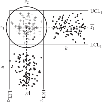
Projecting the samples of the individual charts into the central box between both charts yields a scatter diagram. The scatter points marked by ‘+’ are the intercept of the projections associated with the same sample index, e.g. z1(k) and z2(k) represent the kth point in the scatter diagram. The confidence region for the scatter diagram can be obtained from the joint PDF. Defining f1( · ) and f2( · ) as the PDF of z1 and z2, respectively, and given that r12 = 0 the joint PDF f( · ) is equal to1
The joint PDF in (1.10) can also be written in matrix-vector form
where
1.12 ![]()
is the covariance matrix of ![]() and
and ![]() and | · | is the determinant of a matrix.
and | · | is the determinant of a matrix.
In a similar fashion to the covariance matrix, the correlation between a set of nz variables can be described by the correlation matrix. Using (1.8) for i = j, the diagonal elements of this matrix are equal to one. Moreover, the non-diagonal elements possess values between − 1 ≤ rij ≤ 1. The concept of correlation is also important to assess time-based trends within the process variables. However, the application of MSPC assumes that the process variables do not possess such trends.
Based on (1.11), a confidence region can be obtained as follows. Intercept a plane located close and parallel to the z1 − z2 plane with f(z1, z2). The integral over the interception area hugging the joint PDF is equal to 1 − α. The contour describing this interception is defined as the control ellipse and represents the confidence region. It should be noted that if the variance of both variables are identical, the control ellipse reduces to a circle, which is the case described in Figure 1.6.2 Subsection 1.2.3 shows how to construct a control ellipse.
One could naively draw a ‘rectangular’ confidence region that is bounded by the upper and lower control limits of the individual Shewhart charts. Since the individual samples are all inside the upper and lower control limits for both charts, the scatter points must fall within this ‘rectangle’. By directly comparing the ‘rectangle’ with the control ellipse in Figure 1.6, it can be seen both areas are comparable in size and that the scatter points fall within both.
The four corner areas of the rectangle that do not overlap with the circular region are small. Statistically, however, the circular region is the correct one, as it is based on the joined PDF. The comparison between the ‘rectangle’ and the circle, however, shows that the difference between them is negligible. Thus, the individual and joint analysis of both process variables yield an in-statistical-control situation.
1.2.2 Perfectly correlated variables
In this second case, the two variables ![]() and
and ![]() have a correlation coefficient of − 1. According to (1.8), this implies that the covariance σ122 is equal to
have a correlation coefficient of − 1. According to (1.8), this implies that the covariance σ122 is equal to
1.13 ![]()
For identical variances, σ12 = σ22 = σ2, it follows that
1.14 ![]()
In other words, ![]() . For unequal variances, both signals are equal up to the scaling factor
. For unequal variances, both signals are equal up to the scaling factor ![]() . Figure 1.7 shows the Shewhart charts for z1 and z2 which are plotted horizontally and vertically, respectively. Given that both variables have the same variance, both of them produce identical absolute values for each sample. This, however, implies that the projections of each sample fall onto a line that has an angle of 135° and 45° to the abscissas of the Shewhart chart for variable z1 and z2, respectively.
. Figure 1.7 shows the Shewhart charts for z1 and z2 which are plotted horizontally and vertically, respectively. Given that both variables have the same variance, both of them produce identical absolute values for each sample. This, however, implies that the projections of each sample fall onto a line that has an angle of 135° and 45° to the abscissas of the Shewhart chart for variable z1 and z2, respectively.
Figure 1.7 Schematic diagram showing two perfectly correlated variables.
The 2D circular confidence region if ![]() and
and ![]() are statistically uncorrelated therefore reduces to a 1D line if they are perfectly correlated. Moreover, the joint PDF f(z1, z2) in this case is equal to
are statistically uncorrelated therefore reduces to a 1D line if they are perfectly correlated. Moreover, the joint PDF f(z1, z2) in this case is equal to
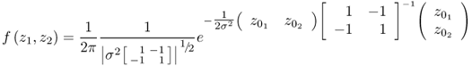
if the variables have equal variance. Equation (1.15), however, presents two problems:
- the determinant of
 is equal to zero; and
 - the inverse of
 therefore does not exist.
This results from the fact that the rank of ![]() is equal to one.
is equal to one.
To determine the joint PDF, Figure 1.8 ‘summarizes’ the scatter diagram of Figure 1.7 by assuming that the control limits for z1 and z2 are ![]() ± 3σ and
± 3σ and ![]() 1 =
1 = ![]() 2 =
2 = ![]() for simplicity. The catheti of the right triangle depicted in Figure 1.8 are the ordinates of both Shewhart charts and the hypotenuse is the semimajor of the ‘control ellipse’. The length of both catheti is 6σ and the length of the hypotenuse is
for simplicity. The catheti of the right triangle depicted in Figure 1.8 are the ordinates of both Shewhart charts and the hypotenuse is the semimajor of the ‘control ellipse’. The length of both catheti is 6σ and the length of the hypotenuse is ![]() , accordingly.
, accordingly.
Figure 1.8 Geometric interpretation of the scatter diagram in Figure 1.7.
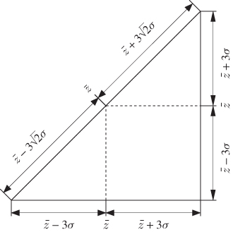
As the projections of the recorded samples fall onto the hypotenuse, the control limits for the projected points are the endpoints of the hypotenuse. Defining the two identical variables z1 and z2 by z the projected samples of z follow a Gaussian distribution and are scaled by 21/2. Next, defining the projected samples of z onto the hypotenuse as t, the ‘joint’ PDF of z1 = z2 = z reduces to the PDF of t
1.16 ![]()
One could argue that only one variable needs to be monitored. An inspection of Figure 1.7, however, yields that the joint analysis is a sensitive mechanism for detecting abnormal process behavior. If the process is in-statistical-control, the sample projections fall onto the hypotenuse. If not, the process is out-of-statistical-control, even if each sample is within the control limits of the individual Shewhart charts. Although a perfect correlation is a theoretical assumption, this extreme case highlights one important reason for conducting SPC on the basis of a multivariate rather than a univariate analysis of the individual variables.
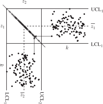
1.2.3 Highly correlated variables
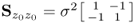
The last two subsections presented two extreme cases for the correlation between two variables. The third case examined here relates to a high degree of correlation between z1 and z2, which is an often observed phenomenon between the recorded process variables, particulary for large-scale systems. For example, temperature and pressure readings, flow rate measurements and concentrations or other product quality measures frequently possess similar patterns. Using a correlation coefficient of −0.95 and unity variance for z1 and z2 yields the following covariance matrix
Figure 1.9 shows, as before, the two Shewhart charts and the scatter diagram, which represents the projected samples of each variable. Given that z1 and z2 are assumed to be normally distributed, the joint PDF is given by
1.18 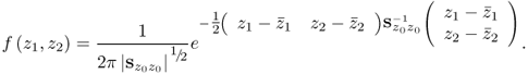
Figure 1.9 Schematic diagram showing two highly correlated variables.
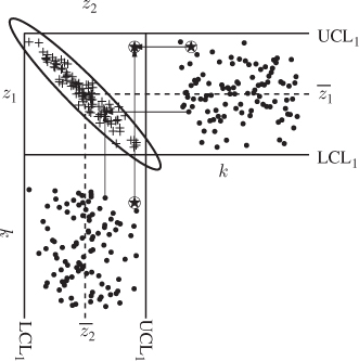
The control ellipse can be obtained by intercepting a plane that is parallel to the z1 − z2 plane to the surface of the joint PDF, such that the integral evaluated within the interception area is equal to 1 − α. Different to two uncorrelated variables of equal variance, this procedure yields an ellipse. Comparing Figures 1.6 and 1.9 highlights that both axes of the circle are parallel to the abscissas of both Shewhart charts for uncorrelated variables, whilst the semimajor of the control ellipse for highly correlated variables has an angle to both abscissas.
1.2.3.1 Size and orientation of control ellipse for correlation matrix 
The following study presents a lucid examination of the relationship between the angle of the semimajor and the abscissa, and the correlation coefficient between z1 and z2. This study assumes that the variance of both Gaussian variables is 1 and that they have a mean of 0. Defining the correlation coefficient between z1 and z2 by r12, produces the following covariance/correlation matrix
1.19 ![]()
It follows from (1.9) that the correlation coefficient is equal to the covariance, since σ12 = σ22 = 1. As discussed in Jackson (2003), the orientation of the semimajor and semiminor of the control ellipse are given by the eigenvectors associated with the largest and the smallest eigenvalue of the ![]() , respectively,
, respectively,
1.20 ![]()
In the above equation, p1 and p2 are the eigenvectors associated with the eigenvalues λ1 and λ2, respectively, and λ1 > λ2.
Eigenvalues of 
For a correlation coefficient ranging from − 1 to 1, Figure 1.10 shows how the eigenvalues λ1 and λ2 depend on the absolute value of the correlation coefficient r12, i.e. λ1(r12) = 1 + |r12| and λ2(r12) = 1 − |r12|. This analysis also includes the two extreme cases discussed in both previous subsections. For r12 = 0, both eigenvalues are equal to 1. On the other hand, if r12 = − 1, the larger eigenvalue is equal to 2 and the other one is 0. The eigenvalues represent the variance of the sample projections on the semimajor (larger eigenvalue) and the semiminor (smaller eigenvalue).
Figure 1.10 Eigenvalues of ![]() , λ1 and λ2, vs. correlation coefficient r12.
, λ1 and λ2, vs. correlation coefficient r12.
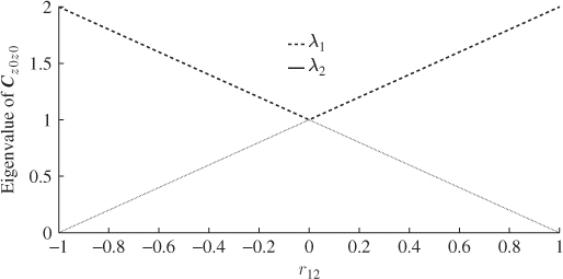
For r12 = 0 the variances of the projected samples onto both axis of the ellipse are identical, which explains why the control ellipse reduces to a circle if σ12 = σ22. For r12 = 1, however, there is no semiminor since all of the projected samples fall onto the hypotenuse of Figure 1.8. Consequently, λ2 is equal to zero (no variance) and the scaling factor between the projections of z, t, and z = z1 = z2 is equal to ![]() since
since ![]() . The introduced variable t describes the distance of the projected point measured from the center of the hypotenuse that is represented by the interception of both abscissas.
. The introduced variable t describes the distance of the projected point measured from the center of the hypotenuse that is represented by the interception of both abscissas.
Orientation of semimajor of control ellipse
The second issue is the orientation of the semimajor relative to the abscissas of both Shewhart charts, which is determined by the direction of ![]() . The angle of the semimajor and semiminor is given by arctan(p21/p11) × 180/π and arctan(p22/p12) × 180/π relative to the z2 axis. This yields the following angles for the ellipse axes:
. The angle of the semimajor and semiminor is given by arctan(p21/p11) × 180/π and arctan(p22/p12) × 180/π relative to the z2 axis. This yields the following angles for the ellipse axes:
1.21 ![]()
and
respectively.
1.2.3.2 Size and orientation of control ellipse for covariance matrix 
In a general case, ![]() , the covariance matrix of z1 and z2, is
, the covariance matrix of z1 and z2, is
1.23 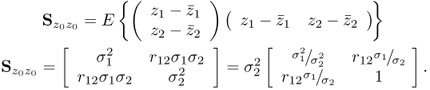
Fixing r12 to, say 0.8, and taking into account that the eigenvectors do not change if this matrix is multiplied by a scalar factor allows examining the effect of ![]() upon the orientation of the eigenvectors. More generally, varying this parameter within the interval
upon the orientation of the eigenvectors. More generally, varying this parameter within the interval ![]() and the correlation coefficient
and the correlation coefficient ![]() as well as defining σ22 = 1 allows examination of:
as well as defining σ22 = 1 allows examination of:
- the angle between p1 and the abscissa; and
- the values of both eigenvalues of
 .
.
Eigenvalues of 
The left plot in Figure 1.11 shows the resultant parametric curves for both eigenvalues vs. ![]() . It is interesting to note that small ratios yield eigenvalues that are close to one for λ1 and zero λ2. This is no surprise given that the variance of z2 was selected to be one, whilst that of z1 is close to zero. In other words, the variance of z2 predominantly contributes to the joint PDF.
. It is interesting to note that small ratios yield eigenvalues that are close to one for λ1 and zero λ2. This is no surprise given that the variance of z2 was selected to be one, whilst that of z1 is close to zero. In other words, the variance of z2 predominantly contributes to the joint PDF.
Figure 1.11 Eigenvalues of ![]() (left plot) and angle of eigenvector associated with larger eigenvalue (right plot) vs.
(left plot) and angle of eigenvector associated with larger eigenvalue (right plot) vs. ![]() and the parameter r12.
and the parameter r12.
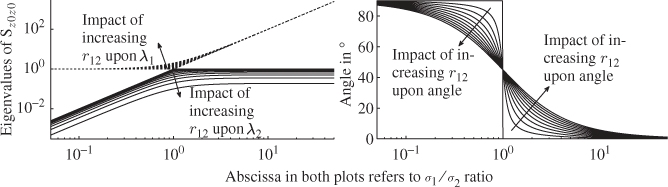
Given that the length of the semimajor and semiminor is proportional to the eigenvalues λ1 and λ2, respectively, the ellipse becomes narrower as the ratio ![]() decreases. In the extreme case of
decreases. In the extreme case of ![]() the control ellipse reduces to a line. On the other hand, larger ratios produce larger values for λ1 and values below 1 for λ2. If no correlation between z1 and z2 exists, that is r12 → 0, the eigenvalue λ2 converges to one for large
the control ellipse reduces to a line. On the other hand, larger ratios produce larger values for λ1 and values below 1 for λ2. If no correlation between z1 and z2 exists, that is r12 → 0, the eigenvalue λ2 converges to one for large ![]() ratios. However, the left plot in Figure 1.11 highlights that λ2 reduces in value and eventually converges to zero if there is a perfect correlation between both variables. For
ratios. However, the left plot in Figure 1.11 highlights that λ2 reduces in value and eventually converges to zero if there is a perfect correlation between both variables. For ![]() , this plot also includes both extreme cases discussed in the previous two subsections. For
, this plot also includes both extreme cases discussed in the previous two subsections. For ![]() , letting r12 → 0 then both eigenvalues are equal to one and r12 = 1, λ1 = 2 and λ2 = 0.
, letting r12 → 0 then both eigenvalues are equal to one and r12 = 1, λ1 = 2 and λ2 = 0.
Orientation of semimajor of control ellipse
The right plot in Figure 1.11 shows how the angle between the semimajor and the abscissa of the Shewhart chart for z1 changes with ![]() and r12. For cases σ1
and r12. For cases σ1 ![]() σ2 this angle asymptotically converges to 90°. Together with the fact that the eigenvalues in this case are λ1 = 1 and λ2 = 0 the control ellipse reduces to a line that is parallel to the abscissa of the Shewhart chart for z1 and orthogonal to that of the Shewhart chart for z2.
σ2 this angle asymptotically converges to 90°. Together with the fact that the eigenvalues in this case are λ1 = 1 and λ2 = 0 the control ellipse reduces to a line that is parallel to the abscissa of the Shewhart chart for z1 and orthogonal to that of the Shewhart chart for z2.
Larger ratios of ![]() produce angles that asymptotically converge to 0°. Given that λ1 converges to infinity and λ2 between zero and one, depending upon the correlation coefficient, the resultant control ellipse is narrow with an infinitely long semimajor that is orthogonal to the abscissa of the Shewhart chart for z1. If r12 → 1, the ellipse reduces to a line.
produce angles that asymptotically converge to 0°. Given that λ1 converges to infinity and λ2 between zero and one, depending upon the correlation coefficient, the resultant control ellipse is narrow with an infinitely long semimajor that is orthogonal to the abscissa of the Shewhart chart for z1. If r12 → 1, the ellipse reduces to a line.
The case of r12 → 0 is interesting, as it represents the asymptotes of the parametric curves. If ![]() the semimajor has an angle of 90°, whilst for values in the range of
the semimajor has an angle of 90°, whilst for values in the range of ![]() , the angle becomes zero. For σ12 = σ22, the control ellipse becomes a circle and a semimajor therefore does not exist.
, the angle becomes zero. For σ12 = σ22, the control ellipse becomes a circle and a semimajor therefore does not exist.
1.2.3.3 Construction of control ellipse
What has not been discussed thus far is how to construct the control ellipse. The analysis above, however, pointed out that the orientation of this ellipse depends on the eigenvectors. The direction of the semimajor and semiminor is defined by the direction of the eigenvectors associated with the larger and the smaller eigenvalues, respectively. The exact length of the semimajor, a, and semiminor, b, depends on the eigenvalues of the covariance matrix
where ![]() is defined by
is defined by
and ![]() is the critical value of a χ2 distribution with two degrees of freedom and a significance α, for example selected to be 0.05 and 0.01.
is the critical value of a χ2 distribution with two degrees of freedom and a significance α, for example selected to be 0.05 and 0.01.
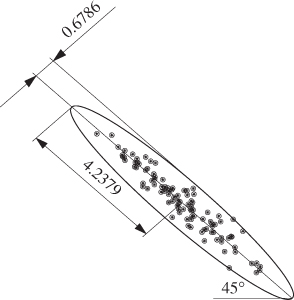
Applying (1.24) and (1.25) to the covariance matrix in (1.17) for α = 0.01 yields ![]() , implying that
, implying that ![]() and
and ![]() . As z1 and z2 have an equal variance of 1, the angle between the semimajor and the abscissa of the Shewhart chart for z2 is 45° as discussed in Equation (1.22). Figure 1.12 shows this control ellipse along with a total of 100 samples of z1 and z2. Jackson (1980) introduced an alternative construction
. As z1 and z2 have an equal variance of 1, the angle between the semimajor and the abscissa of the Shewhart chart for z2 is 45° as discussed in Equation (1.22). Figure 1.12 shows this control ellipse along with a total of 100 samples of z1 and z2. Jackson (1980) introduced an alternative construction
1.26 
Figure 1.12 Control ellipse for ![]() , where
, where ![]() is the covariance/correlation matrix in (1.17), with a significance of 0.01.
is the covariance/correlation matrix in (1.17), with a significance of 0.01.
Based on the preceding discussion, the next subsection addresses the question laid out at the beginning of this section: why multivariate statistical process control?
1.2.4 Type I and II errors and dimension reduction
For the extreme case analyzed in Subsection 1.2.2, it follows that the projections of two perfectly correlated variables fall onto a 1D line and any departure from this line confirms that r12 is no longer equal to 1 for the ‘violating’ samples. Moreover, inspecting Figure 1.9, describing high correlation between two variables with respect to the sample represented by the asterisk yields that this sample shows an in-statistical-control situation, since it is within the control limits of both variables. However, if this sample is analyzed with respect to the multivariate control ellipse it lies considerably outside the normal operating region and hence, describes an out-of-statistical-control situation.
The joint analysis therefore suggests that this sample is indicative of an out-of-statistical-control situation. Comparing this to the case where the two variables are uncorrelated, Figure 1.6 outlines that such a situation can only theoretically arise and is restricted to the small corners of the naive ‘rectangular control region’. Following the introduction of hypothesis testing in Subsection 1.1.3, accepting the null hypothesis although it must be rejected constitutes a Type II error. Figure 1.13 shows graphically that the Type II error can be very substantial.
Figure 1.13 Graphical illustration of Type I and II errors for correlated variable sets.
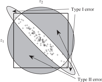
The slightly darker shaded area in this figure is proportional to the Type II error. More precisely, this area represents the difference between the circular and the elliptical confidence regions describing the uncorrelated case and the highly correlated case, respectively. It is interesting to note that correlation can also give rise to Type I errors if larger absolute values for z1 − z2 arise. The brightly shaded areas in Figure 1.13 give a graphical account of the Type I error, which implies that the alternative hypothesis H1, i.e. the process is out-of-statistical-control, is accepted although the null hypothesis must be accepted.
Besides the impact of correlation upon the hypothesis testing, particularly the associated Type II errors, Figure 1.9 highlights another important aspect. Projecting the samples of z1 and z2 onto the semimajor of the control ellipse describes most of the variance that is encapsulated within both variables. In contrast, the remaining variance that cannot be described by projecting the samples onto the semimajor is often very small in comparison and depends on r12. More precisely, the ratio of the larger over the smaller eigenvalue of ![]() is a measure to compute how much the projection of the recorded samples onto the semimajor contribute to the variance within both variables.
is a measure to compute how much the projection of the recorded samples onto the semimajor contribute to the variance within both variables.
A ratio equal to 1 describes the uncorrelated case discussed in Subsection 1.2.1. This ratio increases with r12 and asymptotically describes the case of r12 = 1 which Subsection 1.2.2 discusses. In this case, the variable ![]() , z1 = z2 = z describes both exactly. Finally, Subsection 1.2.3 discuss large ratios of
, z1 = z2 = z describes both exactly. Finally, Subsection 1.2.3 discuss large ratios of ![]() representing large r12 values. In this case, the scatter diagram for z1 and z2 produces a control ellipse that becomes narrower as r12 increases and vice versa.
representing large r12 values. In this case, the scatter diagram for z1 and z2 produces a control ellipse that becomes narrower as r12 increases and vice versa.
In analogy to the perfectly correlated case, a variable t can be introduced that represents the orthogonal projection of the scatter point onto the semimajor. In other words, t describes the distance of this projected point from the origin, which is the interception of the abscissas of both Shewhart charts. The variable t consequently captures most of the variance of z1 and z2. The next chapter introduces data models that are based on approximating the recorded process variables by defining a set of such t-variables. The number of these t-variables is smaller than the number of recorded process variables.
1.3 Tutorial session
Question 1:
What is the main motivation for using the multivariate extension of statistical process control? Discuss the principles of statistical process control and the disadvantage of analyzing a set of recorded process variables separately to monitoring process performance and product quality.
Question 2:
Explain how a Type I and a Type II error affect the monitoring of a process variable and the detection of an abnormal operating condition.
Question 3:
With respect to Figure 1.13, use the area of overlap between the control ellipse and the naive rectangular confidence region, approximate the Type I and II error for using the naive rectangular confidence region for various correlation coefficients, 0 ≤ r12 ≤ 1.
Question 4:
Using a numerical integration, for example the quad2d and dblquad commands in Matlab, determine the correct Type I and II error in Question 2.
Question 5:
Following Questions 2 and 3, determine and plot an empirical relationship between the Type II error and correlation coefficient for two variables.
Project 1:
Simulate 1000 samples from a Gaussian distributed random variable such that the first 500 samples have a mean of zero, the last 500 samples have a mean of 0.25 and the variance of each sample is 1. Determine a Shewhart chart based on the assumption that the process mean is zero and comment on the detectability of the shift in mean from 0 to 0.25. Next, vary the shift in mean and comment on the detectability of the mean.
Project 2:
Construct a CUSUM chart and repeat the experiments in Project 1 for various window lengths. Comment upon the detectability and the average run length of the CUSUM chart depending on the window length. Empirically estimate the PDF of the CUSUM samples and comment on the relationship between the distribution function and the window length with respect to the central limit theorem. Is a CUSUM chart designed to detect small changes in the variable variance? Tip: carry out a Monte Carlo simulation and examine the asymptotic definition of a CUSUM sample.
Project 3:
Develop EWMA charts and repeat the experiments in Project 1 for various weighting parameters. Comment upon the detectability and the average run length depending on the weighting parameter. Is an EWMA chart designed to detect small changes in the variable variance? Tip: examine the asymptotic PDF of the EWMA samples for a change in variance.
Project 4:
Based on the analysis in Projects 2 and 3, study the literature and propose ways on how to detect small changes in the variable variance. Is it possible to construct hypothetical cases where a shift in mean and a simultaneous reduction in variance remains undetected? Suggest ways to detect such hypothetical changes.
1 It follows from a correlation coefficient of zero that the covariance is also zero. This, in turn, implies that two Gaussian distributed variables are statistically independent.
2 Two uncorrelated Gaussian distributed variables that have the same variance describe independently and identically distributed or i.i.d. sequences.