Chapter 7

Monitoring multivariate time-varying processes

As outlined in the first three chapters, MSPC relies on linear parametric PCA or PLS models that are time invariant. Such models, however, may become unrepresentative in describing the variable interrelationships some time after they were identified. Gallagher et al. (1997) pointed out that most industrial processes are time-varying and that the monitoring of such processes, therefore, requires the adaptation of PCA and PLS models to accommodate this behavior. In addition to the parametric models, the monitoring statistics, including their control limits, may also have to vary with time, as discussed in Wang et al. (2003). Another and very important requirement is that the adapted MSPC monitoring model must still be able to detect abnormal process behavior.

Focussing on PCA, this chapter discusses three techniques that allow an adaptation of the PCA model, Recursive PCA (RPCA), Moving Window PCA (MWPCA), and a combination of both. Embedding an adaptive PLS model for constructing the associated monitoring statistics, however, is a straightforward extension and is discussed in Section 7.7. The research literature discussed adaptive PLS algorithms, for example in Dayal and MacGregor (1997c); Helland et al. (1991); Qin (1998); Wang et al. (2003). For the non-causal data representation in (2.2) and the causal ones in (2.24) and (2.51), two properties are of particular interest:

• the speed of adaptation, describing how fast the monitoring model changes with new events; and
• the speed of computation, that is the time the algorithm takes to complete one iteration for model adaptation.

The sensitivity issue, that is how sensitive the adaptive MSPC method is in detecting incipient changes, requires the use of a multiple step ahead application of the currently updating model. In other words, the updated model is not applied when the next sample is available but when the next sample becomes available. This includes the application of the adaptive PCA model as well as the computation of the monitoring statistics and the control limits.

This chapter presents a discussion of the relevant literature on monitoring time-varying processes, followed in Sections 7.2 and 7.3 by a discussion on how to adapt PCA models, which also include the adaptation of the univariate monitoring statistics and their associated control limits. To show the working of an adaptive MSPC model, Sections 7.3, Sections 7.5 and 7.6 summarize application studies to a simulation example, data from a simulated industrial process and recorded data from a furnace process, respectively. Finally, Section 7.8 presents a tutorial session including small projects and questions to help familiarization with this material.

7.1 Problem analysis

The literature has proposed two approaches for updating identified models. The first one is related to a moving window that slides along the data and the other is a recursive formulation. The principle behind the moving window approach is well-known. The window progresses along the data as new observations become available and a new process model is generated by including the newest sample and excluding the oldest one. On the other hand, recursive techniques update the model for an ever-increasing data set that includes new samples without discarding the old ones.

For process monitoring, recursive methods offer efficient computation by updating the process model using the previous model rather than completely building it from the original data (Dayal and MacGregor 1997c; Helland et al. 1991; Li et al. 2000; Qin 1998). Although conceptually simple and successfully employed for process monitoring (Li et al. 2000), Recursive Principal Component Aanalysis (RPCA) may be difficult to implement in practice for the following two reasons:

• the data set on which the model is updated is ever-growing, leading to a reduction in the speed of adaptation as the data size increases. This issue is discussed in Wang et al. (2005); and
• RPCA includes older data that become increasingly unrepresentative of the time-varying process. If a forgetting factor is introduced to down-weight older samples, the selection of this factor can be difficult without a priori knowledge of likely fault conditions.

In comparison, the Moving Window Principal Component Analysis (MWPCA) formulation can overcome some of the above problems by including a sufficient number of data points in the time-window, from which to build the adaptive process model. More precisely, MWPCA allows older samples to be discarded in favor of newer ones that are more representative of the current process operation. Furthermore, the use of a constant size of window results in a constant speed of model adaptation. This, however, may cause a problem when the window has to cover a large number of samples in order to include sufficient process variation for modeling and monitoring purposes since the computational speed of MWPCA then drops significantly. If a smaller window size is attempted to improve computational efficiency, data within the window may then not adequately reveal the underlying relationships between the process variables. An additional danger of a short window is that the resulting model may adapt to process changes so quickly that abnormal behavior may remain undetected.

To improve computational efficiency without compromising the window size, a fast moving window PCA scheme has been proposed by Wang et al. (2005). This scheme relies on the adaptation of the RPCA procedure and yields an MWPCA algorithm for updating (inclusion of a new sample) and downdating (removal of the oldest sample). Blending recursive and moving window techniques has proved beneficial in computing the computation of the discrete Fourier transform and in least-squares approximations (Aravena 1990; Fuchs and Donner 1997).

Qin (1998) discussed the integration of a moving window approach into recursive PLS, whereby the process data are grouped into sub-blocks. Individual PLS models are then built for each data block. When the window moves along the blocks, a PLS model for the selected window is calculated using the sub-PLS models rather than the original sub-block data. The fast MWPCA is intuitively adapted, as the window slides along the original data sample by sample. The general computational benefits of the new algorithm are analyzed in terms of the number of floating point operations required to demonstrate a significantly increased computational efficiency.

Another important aspect worth considering when monitoring a time-varying process is how to adapt the control limits as the process moves on. In a similar fashion to the work in Wang et al (2005, 2003), this chapter uses a -step-ahead horizon in the adaptive PCA monitoring procedure. This implies that the adapted PCA model, including the adapted control limit, is applied after samples are recorded. The advantage of using an older process model for process monitoring is demonstrated by application to simulated data for fault detection. In order to simplify the equations in Sections 7.2 and 7.3 the notation to denote estimates, for example those of the correlation matrix or the eigenvalues, is omitted.

7.2 Recursive principal component analysis

This section introduces the working of a recursive PCA algorithm, which requires:

• the adaptation of the data covariance or correlation matrix;
• a recalculation of the eigendecomposition; and
• an adjustment of the control limits.

The introduction of the RPCA formulation also provides, in parts, an introduction into MWPCA, as the latter algorithm incorporates some of the steps of RPCA derived below. The next section then develops the MWPCA approach along with an adaptation of the control limits and a discussion into suitable methods for updating the eigendecomposition.

The application study in Chapter 7 showed that using the covariance or correlation matrix makes negligible difference if the process variables have a similar variance. Similar observations have also been reported in Jackson (2003). If this is not the case, a scaling is required as the PCA model may otherwise be dominated by a few variables that have a larger variance. This is discussed extensively in the literature. For example, Section 3.3 in reference Jackson (2003) outlines that the entries in the correlation matrix does not have units¹ whereas the covariance matrix may have different units. The same reference, page 65, makes the following remark.

Given that it is preferred to use the correlation matrix, its adaptation is achieved efficiently by adaptively calculating the current correlation matrix from the previous one and the new observation, as discussed in Li et al. (2000). For the original data matrix , which includes n_z process variables collected until time instant K, the mean and standard deviation are given by and . The original data matrix Z is then scaled to produce , such that each variable now has zero mean and unit variance. According to (2.2) and Table 2.1, and the notation results from the scaling to unit variance. The correlation matrix, obtained from the scaled reference data set is accordingly

7.1

Note that the change in subscript from z₀z₀ to 1 is to distinguish between the old correlation matrix from the adapted one, , when the new sample z(K + 1) becomes available. The mean value of the augmented data matrix is given by

7.2

and can be updated as follows

7.3

Again, the subscripts 1 and 2 for the mean vector and the standard deviations are to discriminate between the old and adapted ones. The adapted standard deviation of the ith process variable is

7.4

with . Given that , the centering and scaling of the new sample, z(K + 1), is

7.5

Utilizing , Σ₂, Σ₁, and the old correlation matrix , the updated correlation matrix is given by

7.6

The eigendecomposition of then provides the required new PCA model.

7.3 Moving window principal component analysis

On the basis of the adaptation procedure for RPCA, it is now shown how to derive an efficient adaptation of involving an updating stage, as for RPCA, and a downdating stage for removing the contribution of the oldest sample. This adaptation requires a three step procedure outlined in the next subsection. Then, Subsection 7.3.2 shows that the up- and downdating of is numerically efficient for large window sizes. Subsection 7.3.3 then introduces a -step-ahead application of the adapted MWPCA model to improve the sensitivity of the on-line monitoring scheme. The adaptation of the control limits and the monitoring charts is discussed in Subsections 7.3.4 and 7.3.5, respectively. Finally, Subsection 7.3.6 provides a discussion concerning the required minimum size for the moving window.

7.3.1 Adapting the data correlation matrix

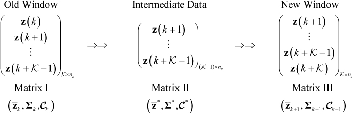
RPCA updates by incorporating the new sample (updating). A conventional moving window approach operates by first discarding the oldest sample (downdating) from the model and then adding the new sample (updating). Figure 7.1 shows details of this two-step procedure for a window size , with k being a sample index. MWPCA is based on this up- and downdating, but incorporates the adaptation developed for RPCA (Li et al. 2000). The three matrices in Figure 7.1 represent the data in the previous window (Matrix I), the result of removing the oldest sample z(k) (Matrix II), and the current window of selected data (Matrix III) produced by adding the new sample to Matrix II. Next, the adaptations of the mean vectors, the standard deviations and the correlation matrices for Matrix II and III are determined.

Step 1: Matrix I to Matrix II

The downdating of the effect of removing the oldest sample from Matrix I can be computed in a similar way to that shown in (7.3).

7.7

Equation (7.8) describes how to downdate the impact of z(k) upon the variable mean

7.8

Using (7.7) and (7.8) the variance of the ith process variable becomes

7.9

and (7.10) stores the standard deviations of the n_z process variables

7.10

Finally, the impact of recursively downdating z(k) from follows from the above equations. For simplicity, the matrix is now introduced to compute

7.11

which can be further divided into

7.12

where

7.13

The downdating for the correlation matrix after elimination of the oldest sample, Matrix II, can now be expressed in (7.14).

7.14

Step 2: Matrix II to Matrix III

This step involves the updating of the PCA model by incorporating the new sample. Based on (7.3) and (7.7) the updated mean vector is

7.15

The change in the mean vectors are computed from (7.15) and (7.16)

7.16

and the standard deviation of the ith variable follows from (7.17).

7.17

and (7.18)

7.18

Finally, the scaling of the newest sample, , and the updating of the correlation matrix are described in (7.19)

7.19

and (7.20)

7.20

respectively. Combining Steps 1 and 2 allows deriving Matrix III from Matrix I, the adapted mean, standard deviation and correlation matrix, which is shown next.

Step 3: Combination of Step 1 and Step 2

Including downdating, (7.7), and updating, (7.15), adapting the mean vector directly yields

7.21

The adapted standard deviations follow from combining (7.9) and (7.17)

7.22

where and . Substituting (7.12) and (7.14) into (7.20) produces the adapted correlation matrix of Matrix III

7.23

The combination of Steps 1 and 2 constitutes the fast moving window technique, which is summarized in Table 7.1 for convenience.

Table 7.1 Procedure to update correlation matrix for the MWPCA approach

Step	Equation	Description
1		Mean of Matrix II
2		Difference between means
3		Scale the discarded sample
4		Bridge over Matrix I and III
5		Mean of Matrix III
6		Difference between means
7		Standard deviation of Matrix III
8		Store standard deviations in Matrix III
9		Scale the new sample
10		Correlation matrix of Matrix III

The MWPCA technique gains part of its computational efficiency by incorporating the efficient update and downdate procedures. This is examined in more detail in the Subsection 7.3.3. Subsection 7.3.2 discusses computational issues regarding the adaptation of the eigendecomposition.

7.3.2 Adapting the eigendecomposition

Methods for updating the eigendecomposition of symmetric positive definite matrices have been extensively studied over the past decades. The following list includes the most commonly proposed methods for recursively adapting such matrices:

• rank one modification (Bunch et al. 1978; Golub 1973);
• inverse iteration (Golub and van Loan 1996; van Huffel and Vandewalle 1991);
• Lanczos tridiagonalization (Cullum and Willoughby 2002; Golub and van Loan 1996; Paige 1980; Parlett 1980);
• first order perturbation (Champagne 1994; Stewart and Sun 1990; Willink 2008);
• projection-based adaptation (Hall et al. 1998, 2000, 2002); and
• data projection method (Doukopoulos and Moustakides 2008).

Alternative work relies on gradient descent methods (Chatterjee et al. 2000) which are, however, not as efficient.

The computational efficiency of the listed algorithms can be evaluated by their number of floating point (flops) operations consumed, which is listed in Table 7.2. Evaluating the number of flops in terms of the order O( · ), that is, is of order , highlights that the data projection method and the first order perturbation are the most economic methods. Given that n_z > n_k, where n_k is the estimated number of source signals for the kth data window, Table 7.2 suggests that the data projection method is more economic than the first order perturbation method. It should be noted, however, that the data projection method:

• adapts the eigenvectors but not the eigenvalues; and
• assumes that the number of source signals, n_k is constant.

If the eigenvectors are known, the eigenvalues can easily be computed as

7.24

Table 7.2 Efficiency of adaptation methods

Adaptation Method	Computational Cost
rank one modification
inverse iteration
Lanczos tridiagonalization
first order perturbation
projection-based
data projection method

If the number of source signals is assumed constant, the additional calculation of the eigenvalues renders the first order perturbation method computationally more economic, since the computation of each adapted eigenvalue is . In practice, the number of source signals may vary, for example resulting from throughput or grade changes which result in transients during which this number of the assumed data model z₀ = Ξs + g can change. Examples of this are available in Li et al. (2000) and 7.6 and 7.7 below. The assumption for the first order perturbation method is that the adapted correlation matrix can be written in the following form

7.25

where is a small positive value. By selecting the above equation represents an approximation of the correlation matrix, since

7.26

On the basis of the above discussion, it follows that:

• an updated and downdated version of the data correlation matrix is available and hence, the adaptation does not need to be part of the adaptation of the eigendecomposition;
• the faster first order perturbation and data projection methods are designed for recursive but not moving window formulations;
• the dominant n_k+1 eigenvectors as well as the eigenvalues need to be adapted;
• the number of retained PCs may change; and
• the algorithm should not be of .

Fast methods for adapting the model and residual subspaces rely on orthogonal projections, such as Gram-Schmidt orthogonalization (Champagne 1994; Doukopoulos and Moustakides 2008). Based on an iterative calculation of a QR decomposition in Golub and van Loan (1996, page 353) the following orthonormalization algorithm can be utilized to determine the adapted eigenvectors:

This algorithm converges exponentially and proportional to (Doukopoulos and Moustakides 2008). Moreover, the computational efficiency is of as discussed in Golub and van Loan (1996, page 232).

The underlying assumption of this iterative algorithm is that the number of source signals, n, is time invariant. In practice, however, this number may vary as stated above. Knowing that the computational cost is , it is apparent that any increase in the number of source signals increases the computational burden quadratically. Applying the following pragmatic approach can account for a varying n:

The adaptation of the eigendecomposition is therefore:

• of O(2n_z(n_k + 1)²) if n_k+1 ≤ n_k; and
• increases to O(2n_z(n_k+1 + 1)²) if n_k+1 > n_k.

The adaptation of the eigenvalues in Step 8 is of . Overall, the number of floating point operations therefore is . Next, we examine the computational cost for the proposed moving window adaptation procedure.

7.3.3 Computational analysis of the adaptation procedure

After evaluating the computational complexity for the adaptation of the eigendecomposition, this section now compares the adaptation using the up- and downdating approach with a recalculation of the correlation matrix using all samples in the new window. The aim of this comparison is to determine the computational efficiency of this adaptation and involves the numbers of floating point operations (flops) consumed for both methods. For determining the number of flops, we assume that:

• the addition and multiplication of two values requires one flop; and
• that factors such as or have been determined prior to the adaptation procedure.

Moreover, the number of flops for products of two vectors and matrix products that involve one diagonal matrix, e.g. (7.22), are of flops and scaling operations of vectors using diagonal matrices, such as (7.19), are of O(n_z).

Table 7.3 presents general algebraic expressions for the number of flops required for updating the correlation matrix in both algorithms. It should be noted that the recalculation of the MWPCA model is of . In contrast, fast MWPCA is only of . The two algorithms can be compared by plotting the ratio of flops consumed by a recalculation over those required by the up- and downdating method. Figure 7.2 shows the results of this comparison for a variety of configurations, that is, varying window length, , and number of variables, n_z.

Table 7.3 Number of flops consumed for adapting correlation matrix

MWPCA technique	Expression
Recomputing correlation matrix
Using up- and downdating approach

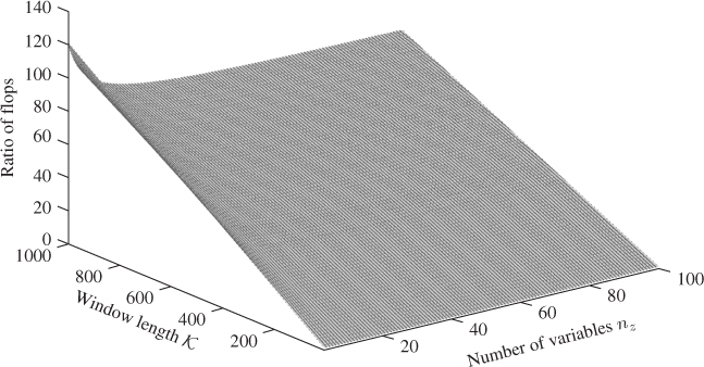
Figure 7.2 shows that the computational speed advantage of the fast MWPCA can exceed 100. The larger the window size, the more significant the advantage. However, with an increasing number of variables, the computational advantage is reduced. Using the expressions in Table (7.3), a hypothetical case can be constructed to determine when the up- and downdating procedure is more economic. For a given number of process variables, a window length that is larger than

7.27

results in a computationally faster execution of the introduced up- and downdating approach. A closer inspection of (7.27) reveals that equality requires the window length to be smaller than n_z if n_z ≥ 10. In order to reveal the underlying correlation structure within the process variables, however, it is imperative to guarantee that . Practically, the proposed up- and downdating method offers a fast adaptation of the correlation matrix that is of . Together with the adaptation of the eigendecomposition, one adaptation step is therefore of . The required adaptation of the control limits is discussed next.

7.3.4 Adaptation of control limits

Equations 3.5 and 3.16 describe how to compute the control limits for both non-negative quadratic statistics. Given that the following parameters can vary:

• the number of retained components, n_k+1; and
• the discarded eigenvalues, , , ···, ,

both control limits may need to be recomputed, as n_k+1 may be different to n_k and the eigenvalues may change too. The number of source signals can be computed by the VRE or VPC criterion for example. The adaptation of the eigendecomposition, however, includes the retained components of the correlation matrix only. Adapted values for the discarded eigenvalues are therefore not available.

The adaptation of Q_α can, alternatively, be carried out by applying 3.29 to 3.31, as proposed by Wang et al. (2003). This has also been discussed in Nomikos and MacGregor (1995) for monitoring applications to batch processes. Equation (3.29) outlines that the parameters required to approximate the control limit, include the first two statistical moments of the Q statistic

7.28

A moving window adaptation of these are given by:

7.29

to estimate the mean and

7.30

for the variance. Here

• ; and
• .

After computing _k+1 and , the parameters g_k+1 and h_k+1 can be calculated

7.31

After developing and evaluating the moving window adaptation, the next subsection shows how to delay the application of the adapted PCA model.

7.3.5 Process monitoring using an application delay

The literature on adaptive modeling advocates the application of adapted models for the next available sample before a readaptation is carried out. This has also been applied in earlier work on adaptive MSPC (Lee and Vanrolleghem 2003; Li et al. 2000; Wang et al. 2003). The adaptation of each variable mean and variance as well as the correlation matrix, however, may allow incipient faults to be adapted. This may render such faults undetectable particulary for small window sizes and gradually developing fault conditions. Increasing the window size would seem to be a straightforward solution to this problem. Larger window sizes, however, result in a slower adaptation speed and changes in the variable interrelationships that the model should adapt may consequently not be adequately adapted. Therefore, the adaptation using a too large window has the potential to produce an increased Type I error.

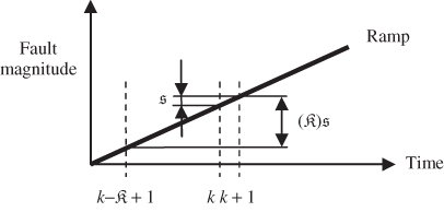
To prevent the adaptation procedure from adapting incipiently developing faults Wang et al. (2005) proposed the incorporation of a delay for applying the adapted PCA model. More precisely, the previously adapted PCA model is not applied to analyze the next recorded sample. Rather, it is used to evaluate the sample to be recorded time steps later. Figure 7.3 exemplifies this for an incipient fault described by a ramp. When the (k + 1)th sample becomes available, the model which is adapted by including the th and discarding the th samples is used to monitor the process, rather than the one including the kth and discarding the th samples. As Figure 7.3 illustrates, the older model is more sensitive to this ramp-type fault since the recent model is likely to have been corrupted by the samples describing the impact of the ramp fault.

Incorporating the -step-ahead application of the monitoring model results in the following construction of the Hotelling's T² statistic

7.32

Both and are obtained from the th model, while is the (k + 1)th sample scaled using the mean and variance for that model, that is, . The Q statistic for this sample is

7.33

It should be noted that a one-step-ahead prediction corresponds to . Another advantage of the application delay is the removal of samples that lead to Type I errors for both univariate statistics. Such violating samples are earmarked and excluded from the adaptation process. This can further prevent samples describing incipient faults to corrupt the monitoring model. The increase in sensitivity for detecting incipient fault conditions for is demonstrated in the next three sections.

7.3.6 Minimum window length

This issue relates to the minimum number of samples required to provide a sufficiently accurate estimate of the data covariance matrix from the data within the sliding window. Following from the discussion in Section 6.4, if the window size is small, the variances for estimating the mean and variance/covariance is significant.

The number of samples required to estimate the variance of a single variable has been extensively discussed in the 1950s and early 1960s (Graybill 1958; Graybill and Connell 1964; Graybill and Morrison 1960; Greenwood and Sandomire 1950; Leone et al. 1950; Tate and Klett 1959; Thompson and Endriss 1961). Based on this early work, Gupta and Gupta (1987) derived an algorithmic expression to determine the required sample size for multivariate data sets.

For a Gaussian distributed variable set, if the variable set is independently distributed, that is, the covariance matrix is a diagonal matrix, the minimum number of samples is approximately , where , α is the significance, ε is the relative error and defines the confidence interval of a zero mean Gaussian distribution of unity variance. As an example, to obtain the variance of n_z = 20 independently distributed (i.d.) variables for ε = 0.1 and α = 0.05 requires a total of samples. Table 2 in Gupta and Gupta (1987) provides a list of required samples for various configurations of n_z, ε and α.

In most practical cases, it cannot be assumed that the covariance matrix is diagonal, and hence the theoretical analyses in the previous paragraph are only of academic value. However, utilizing the algorithm developed in Russell et al. (1985), Gupta and Gupta (1987) showed that writing the elements of the covariance matrix and its estimate in vector form, that is, and with σ₂₁² = r₁₂ σ₁ σ₂ and its estimate, allows defining the random vector , since a covariance matrix is symmetric.

The vector , where the elements of are (Muirhead 1982). For a given ε and α and the definition of , the probability 1 − α can be obtained through integration of

As the limits of the integration depend on the number of samples, the integral can be evaluated using the algorithm proposed by Russell et al. (1985).

It is important to note, however, that the resultant size of the reference sample depends on , which is usually unknown. Despite this, the analysis of the integral allows the following conclusions to be drawn: (i) an increase in the number of recorded variables yields a larger size of as well and (ii) highly correlated variables may require a reduced reference set.

These conclusions follow from the discussion in Gupta and Gupta (1987). Particularly the last point, that a increasing degree of correlation among the process variables may lead qualitatively to a reduction in the number of samples required, is of interest. The preceding discussion therefore highlights that window size does not only depend on the size of the variable set. Given that the variables of industrial processes are expected to possess a high degree of correlation implies that window size may not necessarily increase sharply for large variable sets.

Another, more pragmatic, approach is discussed in Chiang et al. (2001), which relies on the estimation of the critical value for the Hotelling's T² statistic. As discussed in Subsection 3.1.2, assuming the data covariance matrix is known, the Hotelling's T² statistic follows a χ² distribution and the critical value is given by . On the other hand, if the data covariance matrix needs to be estimated, the Hotelling's T² statistic follows an F-distribution, for which the critical value can be obtained as shown in (3.5). Tracey et al. (1992) outlined that the critical value of an F-distribution asymptotically converges to that of a χ² distribution, that is:

7.34

Defining the relative difference between both critical values

7.35

which gives rise to

7.36

and can be solved by iteration. Here, . Table 2.2 in Chiang et al. (2001) lists solutions for various values of n_z with ϵ and α being 0.1 and 0.05, respectively. The minimum number of required samples in this table suggests that it should be roughly 10 times the number of recorded variables. Chiang et al. (2001) highlighted that this pragmatic approach does not take the correlation among the process variables into account and may yield a minimum number that is, in fact, too small. More precisely, Section 11.6 in Anderson (2003) describes that confidence limits for eigenvalues and eigenvectors depend on .

As control limits for the Q statistic, however, depend on the discarded eigenvalues, which follows from (3.16), inaccurately estimated discarded eigenvalues may have a significant and undesired impact upon the computation of Q_α. This implies that the number suggested in (7.36) may be sufficient to determine an appropriate minimum number for constructing the control limit for the Hotelling's T² statistic. However, a significantly larger number may be required in order to prevent erroneous results for computing the control limit of the Q statistic.

The suggested value can therefore be used as a guideline knowing that it is advisable to opt for a larger . As the above discussion and the analysis in Section 6.4 highlight, the number of samples required to construct accurate estimates of the data covariance/correlation matrix is still an open issue for the research community.

7.4 A simulation example

This section studies the delayed application of an adaptive MSPC monitoring model using a simulated process. The example process is designed to represent slowly changing behavior in the form of a ramp. Such situations are common in industrial practice and include leakages, pipe blockages, catalyst degradations, or performance deteriorations in individual process units. If an adaptive MSPC monitoring approach is applied in this scenario, such gradual and incipient changes may be accommodated by model adaptation and hence remain unnoticed.

The aim of this section is therefore to study whether the proposed adaptation can detect such incipient faults. A description of the simulated process is given first, followed by an application of a standard PCA-based monitoring model in Subsection 7.4.2. Finally, Subsection 7.4.3 then shows the application of MWPCA and studies the impact of an application delay.

7.4.1 Data generation

The process has four process variables and is based on the following data structure

7.37

Each of the above variables follow a Gaussian distribution, with

7.38

for the source variables and

7.39

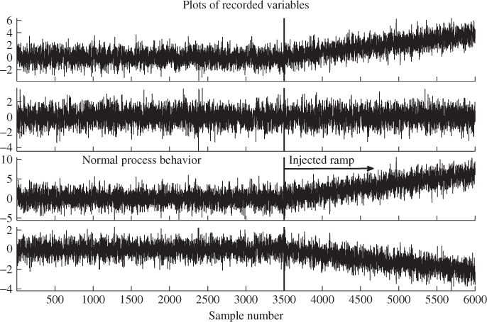
for the error variables. Moreover, the source and error variables are independent, that is, . From this process, a total of 6000 samples were generated. To simulate an incipient fault condition, a ramp with a slope of 0.0015 between two samples was superimposed on the first source variable from sample 3501 onwards

7.40

The relationships between the variables, i.e. Ξ and , remain unchanged. Thus, the orientation of the model subspace or the residual subspace did not change over time. The simulated process could therefore be regarded as changing to a different, and undesired operating region. Figure 7.4 shows plots of the four process variables for the entire data set. Utilizing this data set for monitoring the simulated process allows us to demonstrate that a varying application delay can:

• accommodate the injected ramp by considering this change as normal; or
• consider this ramp as a process fault that must be detected.

This is discussed in Subsection 7.4.3, following an application of PCA.

7.4.2 Application of PCA

Concentrating on , the scaling does not affect the error covariance matrix with . Hence the two discarded eigenvalues are 0.1. Moreover, none of the elements in changed. This implies that the orientation of the model subspace is not affected by the fault condition. Secondly, (3.7) outlines that the Q statistic is not affected either, since the error vector remains unchanged. Hence, neither the orientation of the residual subspace nor the variance of the discarded principal components changed.

In fact, the first n score variables predominantly describe the variation of the source signals, which follows (2.8). With this in mind, the Q statistic describing the fault condition, Q_f, becomes

7.41

and hence

7.42

which implies that Q_f(k) = Q(k) ≤ Q_α. The above relationship utilized the fact that:

• the source and error variables are uncorrelated;
• the model subspace, spanned by the column space of Ξ, is orthogonal to the residual subspace spanned by the column vectors of P_d; and
• the abnormal condition is described here by

The same analysis for the Hotelling's T² statistic yields

7.43

The above equation shows that the ramp-type fault has two effects upon the T² statistic. The term describes a parabola of the form

7.44

The second term is a Gaussian distributed contribution with a quadratically increasing variance,

7.45

To determine the parameters and , we need the first two eigenvector-eigenvalue pairs of the covariance matrix corresponding to the example process described in (7.37) to (7.40)

7.46

which has the following dominant eigenpairs

7.47a

7.47b

With , the parameters and are equal to

7.48

When the ramp-type fault is injected for a total of 2500 samples, that is, from sample 3501 to the end of the simulated set, the parabola has a height of 2.4101 × 10⁻⁶ × 2500² = 15.0634 and the standard deviation of is . It is interesting to note that the parameters and are equal up to a scaling factor of 4. In other words the height of the quadratic term is one fourth of the variance of .

Figure 7.5 plots both monitoring statistics for the 6000 simulated samples. Whilst the first 3000 samples served as a reference data set to identify a PCA model including the construction of the monitoring statistics and their control limits, this monitoring model was applied to entire data set. For the first 3500 samples, both statistics described normal process behavior. After the injection of the fault, significant violations of the T² statistic arose from around the 4200th sample onwards, whilst the Q statistic remained insensitive to the fault.

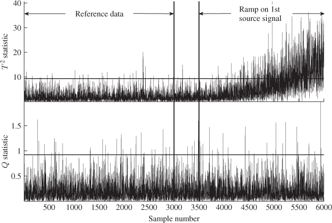
This suggests a delay in detecting this event of about 700 samples. In SPC, such a delay is often referred as the average run length, that is, the difference in which a process commences to run at a normal operating condition and that at which the monitoring scheme indicates a change from acceptable to rejectable quality level. According to (7.43) to (7.45), the ramp will augment the T² statistic by superimposing a quadratic bias term and normally distributed sequence which increases in variance as the fault becomes more severe. This can be confirmed by inspecting the upper plot in Figure 7.5. The next subsection studies the influence of a -step-ahead application of an adapted model.

7.4.3 Utilizing MWPCA based on an application delay

To illustrate the effect of applying the adapted MSPC monitoring model with a delay of samples is now studied. Commencing with the traditional approach, Figure 7.6 shows both monitoring statistics for a window length of . By closer inspection, the number of Type I errors does not exceed 1% and hence, the injected ramp-type fault cannot be detected. Moreover, the lower two plots give a clear picture when the null hypothesis, that the process is in-statistical-control, is accepted (value of zero) or when this hypothesis is rejected (value of one).

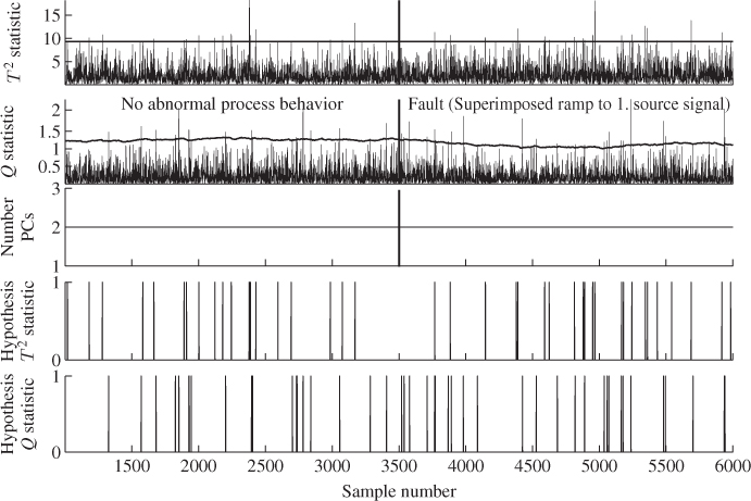
Besides the Type I error being close to 1%, the hypothesis plots for the T² and Q statistics do not indicate a higher density of rejections of the null hypothesis between samples 3500 and 6000. If we assume that such behavior is a normal occurrence, for example the performance deterioration of an operating unit, and the adaptive monitoring model should accommodate this behavior, selecting the values for and is appropriate.

The middle plot in Figure 7.6 shows how the estimated number of source signals vary over time. This number was estimated using the VRE technique, described in Subsection 2.4.1. Since the injected fault does not affect the geometry of the PCA model subspace nor the residual subspace, the number of source signals does not change. Hence, the adaptation procedure constantly determines, as expected, that two latent component sets are sufficient.

However, if we do not consider this behavior normal then the selection of both parameters will render this fault consequently undetectable. The preceding analysis showed that an increase in will reduce the impact of new samples upon the covariance/correlation matrix. With reference to (7.11), (7.12), (7.14), (7.20) and (7.23) this follows from the fact that and asymptotically converge to 1 and 0 as , respectively.

On the other hand, Figure 7.4 shows that a delayed application of the adapted MSPC model may increase the impact of a fault upon the process performance samples earlier. Selecting and to be 2000 and 100, Figure 7.7 shows that the ramp-type fault can now be detected. Comparing the lower two plots in Figure 7.7 with those of Figure 7.6 yields a statistically significant number of violations of the Hotelling's T² statistic between samples 3500 and 6000.

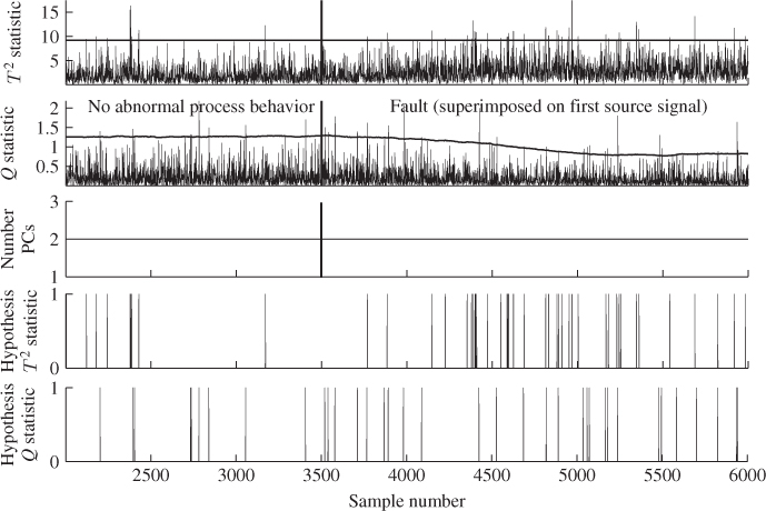
The empirical significance level is now 1.4% which indicates an out-of-statistical-control performance. In contrast, the number of violations of the Q statistic for the same data section is close to 1% and hence this statistic suggests we should accept the hypothesis that the process is in-statistical-control. Altering the window length and the application delay allows studying the influence of both parameters upon the sensitivity in detecting the ramp-type fault.

Table 7.4 presents the result of such an analysis where the empirical significance is determined for the number of violations for the data range 3001 to 6000 and divided by the total number of 3000 samples. By browsing through the columns of this table, it is interesting to note that the empirical significance for the Q statistic in any configuration is very close to the 1%. Following the analysis in (7.42), this is expected since the fault does not affect the Q statistic.

Table 7.4 Results of -step-ahead application for various window lengths .

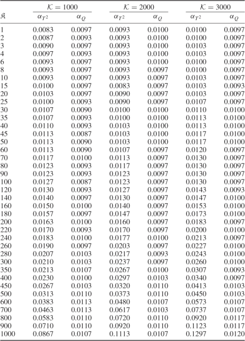
For a better visualization of the results in Table 7.4, Figure 7.8 shows the constant number of Type I errors for the Q statistic in any configuration. With regards to the T² statistic, a different picture emerges. As expected, the larger the window length the less new samples affect the adaptation of the monitoring model. In Figure 7.4, the dash-dot line represents a window length of , which confirms this.

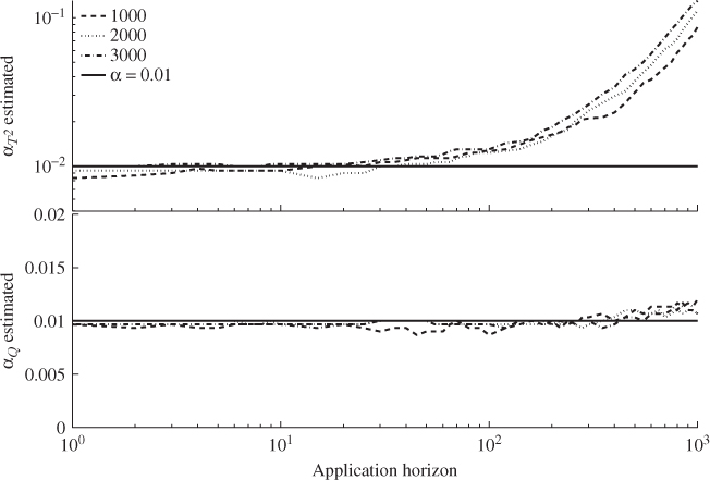
The figure also shows that increased empirical significance levels for emerged for an application horizon of . For and , the sensitivity in detecting this fault condition decreases. A clear and increasing empirical significance level can be noticed for . The increases for the latter two configurations are also not as pronounced as for the window length of .

7.5 Application to a Fluid Catalytic Cracking Unit

This section applies the adaptive monitoring scheme to a realistic simulation of a Fluid Catalytic Cracking Unit (FCCU) that is described in McFarlane et al. (1993). This application is intended to include incipient time-varying behavior that represents a normal operational change and a second more pronounced process fault. Both conditions take the shape of a ramp, where the adaptive monitoring approach must incorporate the first change in order to prevent false alarms. In contrast, the adaptive monitoring approach must be able to detect the second change. A detailed description of this process is given next, prior to a discussion of how the data was generated and how the adaptive monitoring model was established in Subsection 7.5.2. Then, Subsection 7.5.3 presents a pre-analysis of the simulated data set. This is followed by describing the monitoring results using PCA and MWPCA with an application delay of one instance in Subsections 7.5.4 and 7.5.5, respectively.

7.5.1 Process description

An FCCU is an important economic unit in oil refining operations. It typically receives several heavy feedstocks from other refinery operations and cracks these streams to produce lighter, more valuable components that are eventually blended into gasoline and other products. Figure 7.9 presents a schematic diagram of this particular Model IV FCCU, which is similar to that in McFarlane et al. (1993).

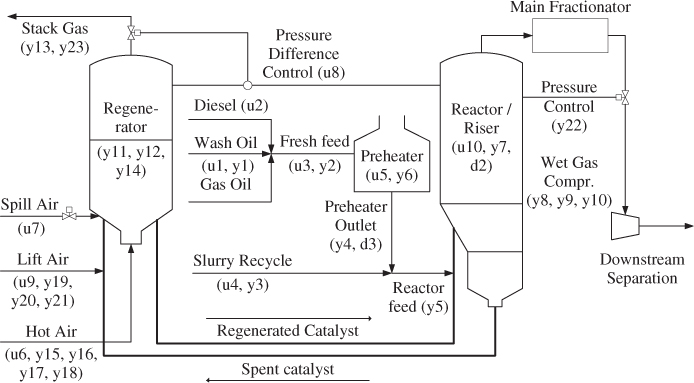
The principal feed to the FCCU is gas oil, but heavier diesel and wash oil streams also contribute to the total feed stream. This fresh feed is preheated in a furnace and then passed to the riser, where it is mixed with hot, regenerated catalyst from the regenerator. In addition to the feed stream, slurry from the main fractionator bottoms is also recycled to the riser. The hot catalyst from the regenerator provides the heat necessary for the endothermic cracking reactions. These produce gaseous products which are passed to the main fractionator for separation. Wet gas off the top of the main fractionator is elevated to the pressure of the light ends plant by the wet gas compressor. Further separation of light components occurs in this light ends separation section that are not included in this simulation model.

As a result of the cracking process inside the reactor, a carbonaceous material, known as coke, is deposited on the surface of the catalyst. Since the deposited coke depletes the catalyst property, spent catalyst is recycled to the regenerator where it is mixed with air in a fluidized bed for regeneration of its catalytic properties. The regeneration occurs when oxygen reacts with the deposited coke to produce carbon monoxide and carbon dioxide. The air is provided by a high-capacity combustion air blower and a smaller lift air blower. In addition to contributing to the combustion process, air from the lift air blower assists with the catalyst circulation between the reactor and the regenerator. Complete details of the mechanistic simulation model for this particular model IV FCCU can be found in McFarlane et al. (1993) including a complete list of recorded variables.

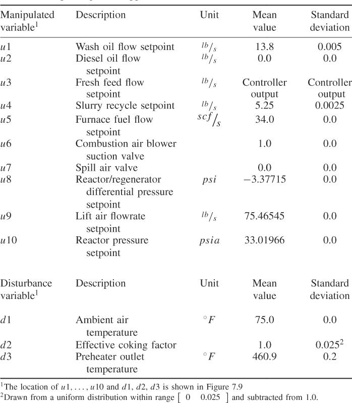
The input variables of the FCCU simulator are listed in McFarlane et al. (1993, page 288, Table 3). Table 7.5 summarizes the construction of the input sequences to generate the data that were used in this study. In addition to a number of regulatory controllers, the riser temperature in the reactor was controlled to a setpoint of 985°F using a PI controller. This controller determines the setpoint value for the total fresh feed. For the kth sample, the controller output is determined by the setpoint error e_Riser(k), which is the difference between the setpoint value of 985°F and the actual measurement of the riser temperature, the integral over the setpoint error, here approximated using a numerical integration based on the trapezoidal rule, and an offset of 126.0 lb/s

7.49

Applying a variety of standard tuning rules, suitable values for the controller parameter K_P and K_I were found to be −0.105 and −0.01, respectively, and T_S is the sampling time of 1 minute.

Table 7.5 Input sequences applied to FCCU simulator

7.5.2 Data generation

The FCCU simulator provides readings for a total of 36 variables, listed on page 289 in McFarlane et al. (1993) (Table 4). From these, 23 variables, listed in Table 7.6, were included in the subsequent analysis and form the data vector z. The excluded 13 variables were constant and hence did not offer any information for monitoring the unit. The FCCU system was simulated for a sampling frequency of once per minute. The controller interaction to maintain the riser temperature at 985°F also occurred at a sampling interval of 1 minute. In order to simulate measurement noise, each of the recorded variables was superimposed by independently distributed noise sequences that followed a Gaussian distribution. These sequences had a mean of zero and a variance of 5% to that of the uncorrupted variable.

Table 7.6 Process variables included in the analysis of the FCCU.

Variable1	Description	Unit
y1 = z1	Flow of wash oil to reactor riser
y2 = z2	Flow of fresh feed to reactor riser
y3 = z3	Flow of slurry to reactor riser
y4 = z4	Temperature of fresh feed entering furnace	°F
y5 = z5	Temperature of fresh feed entering reactor riser	°F
y6 = z6	Furnace firebox temperature	°F
y7 = z7	Temperature of reactor riser	°F
y8 = z8	Wet gas compressor suction pressure	psia
y9 = z9	Wet gas compressor inlet suction flow	ICFM
y10 = z10	Wet gas flow to the vapor recovery unit
y11 = z11	Temperature of regenerator bed	°F
y12 = z12	Regenerator pressure	psia
y13 = z13	Concentration of oxygen in regenerator stack gas	mole%
y14 = z14	Level of catalyst in standpipe	ft
y15 = z15	Combustion air blower inlet suction flow	ICFM
y16 = z16	Combustion air blower throughput
y17 = z17	Combustion air flow to the regenerator
y18 = z18	Combustion air blower discharge pressure	psia
y19 = z19	Lift air blower inlet suction flow	ICFM
y20 = z20	Actual speed of the lift air blower	RPM
y21 = z21	Lift air blower throughput
y22 = z22	Wet gas compressor suction valve position
y23 = z23	Stack gas valve position

¹ The location of the recorded variables y1, … , y23 is shown in Figure 7.10

In this configuration, 15 000 samples were recorded. The two abnormal conditions were a deteriorating performance of the furnace and a fault in the combustion air blower. The next two subsections summarize the effects of these conditions by analyzing the mechanistic model in McFarlane et al. (1993).

7.5.2.1 Injecting a performance deterioration of the furnace

This is a naturally occurring phenomena that is practically addressed through a routine maintenance of the unit. The effect of a performance deterioration can be felt in the enthalpy balance within the furnace. The main variables affected are the furnace firebox temperature and the fresh feed temperature to the riser. This behavior describes a performance deterioration in heat exchangers and translated into a decrease in the furnace overall heat transfer coefficient UA_f. According to McFarlane et al. (1993, page 294), the change in UA_f affects the temperature within the firebox, T₃, through the following enthalpy balance

7.50

where:

• τ_fb = 200s is the furnace firebox time constant;
• F₅ is the fuel gas flow to the furnace in ;
• is heat of combusting the furnace fuel;
• is the log mean temperature difference;
• T₁ = 460.9°F is the fresh feed temperature entering the furnace;
• T₂ is the fresh feed temperature entering the reactor in °F;
• T₃ is the furnace firebox temperature in °F; and
• Q_loss is the heat loss from the furnace in .

The analysis in McFarlane et al. (1993) also yields that T₂ is affected by alterations of the parameter UA_f

7.51

where:

• τ_fo = 60s is the furnace time constant;
• ; and
• F₃ is the flow of fresh feed to the reactor.

This naturally occurring deterioration was injected after the first 5000 samples were recorded. The change in the parameter UA_f was as follows

7.52

It is important to note that the deteriorating performance of units is dealt with by routine inspections and scheduled maintenance programs. For process monitoring, this implies that the on-line monitoring scheme must adapt to performance deterioration like this one unless this deterioration directly affects the product quality or has an adverse effect upon other operation units. On the other hand, the monitoring scheme must be sensitive in detecting fault conditions, for example in individual units, and correctly reveal their progression through the process so that experienced plant operators are able to identify the root causes of such events and respond appropriately. The generated data set included the injection of a fault located in the combustion air blower that is discussed next.

7.5.2.2 Injecting a loss in the combustion air blower

This fault was a gradual loss in the air blower capacity for any number of reasons. The discussion in McFarlane et al. (1993) outlines that this fault affects the combustion air blower throughput as follows

7.53

Here

• F₆ is the combustion air blower throughput in ;
• p₁ is the combustion air blower suction pressure in psia;
• F_surca = 45, 100ICFM is the combustion air blower inlet suction flow; and
• T_atm is the atmospheric temperature of 75°F.

The fault condition was injected after 10 000 samples were simulate by altering the coefficient as follows:

7.54

Note that the constant includes conversions from to (ICFM) and from to (psia). A change in F₆ affects an alteration of the combustion air blower suction pressure, p₁

7.55

and the combustion air blower discharge pressure, p₂

7.56

where κ₁ and κ₂ are constants (McFarlane et al. 1993) if the atmospheric temperature is assumed to be constant and , and F₇ are the flows through the combustion air blower suction valve and combustion air blower vent valve, and the combustion air flow to the regenerator in , respectively, and are given by

7.57

Here, p_rbg = p₆ + κ₆W_reg is the pressure at the bottom of the regenerator, κ₃ to κ₆ are constants, p_atm is the atmospheric pressure (assumed constant), p₆ is the regenerator pressure and W_reg is the inventory of catalyst in the regenerator. It is important to note that (7.55) to (7.57) are interconnected. For example, p₁ is dependent upon and vice versa. In fact, most of the variables related to the combustion air blower are affected by this fault, including the combustion air blower suction flowrate F_succa

7.58

Within the regenerator, a change in the combustion air flow to the regenerator affects the operation of the smaller lift air blower, including the lift air blower speed, s_a

7.59

where V_lift is the lift air blower steam valve, which regulates the total air flow to the regenerator, F_T = F₇ + F₉ + F₁₀. This, in turn, implies that this minor fault in the combustion air blower does not affect the reacting conditions in the regenerator. Other variables of the lift air blower that are affected by a change in the lift air blower speed include the lift air blower suction flowrate, F_sucla

7.60

where s_b is the base speed of the lift air blower and F_base is the air lift compressor inlet suction flow at base conditions and lift air blower throughput, F₈

7.61

7.5.3 Pre-analysis of simulated data

The analysis of this unit involved a total of 23 variables, shown in Table 7.6. Figure 7.10 shows the recorded data set including the performance deterioration of the furnace and the fault in the combustion air blower. In this figure, the variables are plotted in the order they are listed in Table 7.6: the upper left plot depicts the first six variables, the upper right plot shows variables 7 to 12, the lower left plot presents variables 13 to 18 and the lower right plot charts the remaining variables.

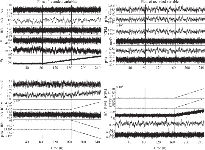
Following the analysis of the fault conditions in Subsection 7.5.2, the performance deterioration of the furnace affected the temperature of fresh feed entering reactor riser, variable 5, and the furnace firebox temperature, variable 6. Inspecting the middle section of the plots in Figure 7.10, data points 5001 to 10 000, these are indeed the only two variables that showed an effect on the performance deterioration. However, the fresh feed temperature to the riser was hardly affected although a minor negative trend can be noticed in Figure 7.10. Concentrating on the right section of the simulated data, data points 10 001 to 15 000, affected by the fault in the combustion air blower are variables 14 to 21.

With regards to the underlying mechanistic model of the FCCU in the previous subsection, the recorded variables confirmed that the effect of this fault was mainly felt in both air blowers but did not have a noticeable impact in the regenerator and hence the reactor riser. The impact upon the catalyst level in the standpipe, variable 16 can be attributed to the increase in spill air, and lift air had a minor effect on the catalyst circulation between the reactor and the regenerator. That a loss in combustion air blower capacity resulted in a reduction in combustion air blower output, including the throughput, F₆, the air flow to the regenerator, F₇, and the discharge pressure, p₂, makes sense physically.

The increase in the combustion air blower inlet suction flow, however, is more difficult to explain. A close inspection of (7.53), (7.55), (7.56) and (7.58) yields that the alterations in the parameter led to a constantly changing operating point. More precisely, (7.58) suggests that the suction flowrate could only increase if p₂ decreased and p₁ increased or remained constant. In fact, the pressure p₁ remained constant and was, as discussed above, therefore not included in this analysis. Consequently, F_succa increased slightly, as p₂ reduced in value.

According to the model-based analysis in this and the previous subsections, the information encapsulated in the recorded variables revealed a correct signature of the combustion air blower fault as well as the naturally occurring performance deterioration of the furnace. The next two subsections present the application of PCA and the discussed MWPCA approach to detect and diagnose both events.

7.5.4 Application of PCA

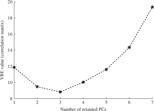
The first step is the identification of a PCA model and involves the estimation of and the number of source signals. The first 5000 samples of the 23 recorded variables described normal process operation and were divided into two sets of 2500 samples. The first 2500 samples were used to obtain the eigendecomposition of the . Figure 7.11 summarizes the results of applying the VRE criterion, detailed in Section 2.4.1, and highlights that the minimum is for three source signals. This implies that recorded variables possess a high degree of correlation.

The second half of the reference set was used to estimate the covariance matrix of the score variables, . It should be noted that an independent estimation of the PCA model and the score covariance matrix is required, which follows from the discussion in Tracey et al. (1992). Figure 7.12 shows the performance of the Hotelling's T² and Q statistics for the entire data set of 15 000 samples. As expected, the first 5000 samples (83 h and 20 min) show the process in statistical control. However, from around 100 h into the data set, excessive violations of the confidence limits arose for both statistics indicating an out-of-statistical-control situation.

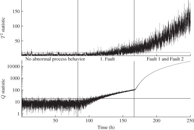
As stated above, however, the data portion representing the middle section of the data (Fault 1), describes a performance deterioration of the furnace which naturally occurs over time. Consequently, it is desirable if the on-line monitoring approach is capable of masking this behavior. Inspecting the performance of the PCA model for the third portion of the data outlines that it can detect both conditions, the performance deterioration in the furnace and the loss in combustion air blower capacity. The application of PCA, therefore, showed an on-line monitoring approach requires to be adaptive in order to accommodate the performance deterioration. The adaptive algorithm, however, must still be able to detect the loss in combustion air blower capacity. Subsection 7.5.4 applies the MWPCA approach to the generated data.

7.5.5 Application of MWPCA

The time-invariant PCA model could detect the presence of both simulated events, which is undesired. The MWPCA method has been designed to adapt the model if the relationship between the recorded process variables is time-variant. The aim of this subsection is to examine whether the performance deterioration of the furnace can be adapted and whether the loss of combustion air blower capacity can be detected.

7.5.5.1 Determining an adaptive MWPCA model

The first step for establishing an adaptive MWPCA model is the selection of window size. For this, 2000 samples were selected to ensure that the data set within the window is large enough to reveal the underlying relationships between the recorded variables. This selection, however, is difficult and presents a tradeoff between the speed of adaptation and the requirement to extract the variable interrelationships of the 23 variables listed in Table 7.6. Table 2.2 in Chiang et al. (2001) suggests that a minimum number of samples is 284 for a total of 25 variables. The discussion in Subsection 7.3.6, however, showed that this number may be too small in the presence of a high degree and estimation of the control limit for the Q statistic. Following the discussion in Subsection 7.3.6, the significantly larger selection for the window size over the suggested one using (7.35) and (7.36) is therefore required.

Figure 7.13 shows the results of applying a MWPCA model for an application delay of . Contrasting Figures 7.13 and 7.12 reveals that utilizing MWPCA removes the excessive number of violations that the PCA model showed in response to Fault 1. The last two plots of Figure 7.13 show the number of violations of the Hotelling's T² and Q statistics. These plots confirm that the number of violations in the first and second portion of the data show an average number of violation of 1% for the Q and around 0.65% of violations for the Hotelling's T² statistic. It can therefore be concluded that MWPCA was able to accommodate the slow performance deterioration in the furnace. However, comparing the last portion of the data, the application of MWPCA could not detect Fault 2, the gradual loss in combustion air blower capacity. This was different with the use of PCA, as Figure 7.12 confirms. It is therefore imperative to rely on the -step ahead application of the currently adapted monitoring model, which is examined next.

7.5.5.2 Utilizing MWPCA based on an application delay

In order to determine the application delay, Subsection 7.4.3 discussed that this parameter can be determined empirically. By selecting , 2, … the empirical significance for the Hotelling's T² and Q statistics can determined for each integer value and listed. Determining from which selected the empirical significance exceeds the selected significance α then provides a threshold. Figure 7.14 summarizes the results of applying a MWPCA model for the selected window size of and a varying number for ranging from 1 to 100.

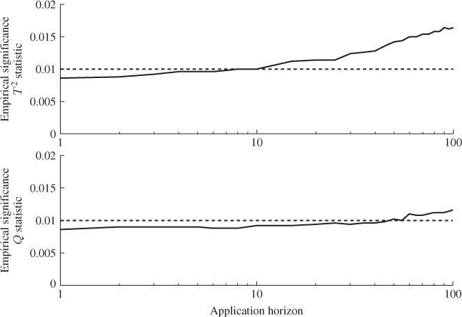
The empirical significance was determined for the first 10 000 samples, which included the first and the middle portion of the data describing the performance deterioration of the furnace. Figure 7.14 highlights that Q statistic produces empirical significance levels between 0.009 and 0.01 for -values below 60. For the Hotelling's T² statistic, -values above ten yield empirical significance values exceeding α = 0.01. Consequently, the application delay was selected to be .

Figure 7.15 shows the performance of the delayed application of the adaptive MWPCA monitoring model. A direct comparison between Figures 7.13 and 7.15 shows that the application delay has no noticeable difference with regards to the number of violations for the first two portions of the data. A difference, though, is the number of source signals. For the first two portions of the data, the VRE criterion determines this number for to be between two and three. In contrast, a constant number of three PCs is suggested for the MWPCA model based on . Different from the utilization of an application delay, each sample was utilized to adapt the MWPCA model including those that produced violations of both univariate monitoring statistics. When adapting the MWPCA model in conjunction with the application delay, samples that produced violations for either statistic were not included.

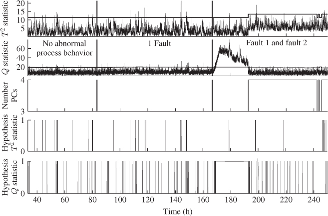
Analyzing the performance of the delayed application of the MWPCA monitoring model to the third section of the data (describing the performance deterioration of the furnace and the loss in combustion air blower capacity) shows that the fault condition can now be detected by the Q statistic. After the first 500 samples violating the Q statistic, was reduced from 10 to 1 and samples that generate violations were again included in the adaptation. This was just after 170 hours into the data set and showed that the MWPCA model could again adapt to both conditions.

After 190 hours, the number of source signals increased to four and the Q statistic did not show significant violations. This implies that both conditions were no longer detectable and is in line with the results of applying MWPCA for a value of one in Figure 7.13. This confirms that setting and excluding samples that produced violations of either statistic made it possible to adapt the naturally occurring performance deterioration. Moreover, the MWPCA monitoring model detected the superimposed process fault describing the loss in combustion air blower capacity.

7.6 Application to a furnace process

This section summarizes the application of PCA and MWPCA based on an application delay to recorded data from a furnace process. The process is briefly described, prior to a summary of the application of PCA to recorded reference data. The section concludes with the application of MWPCA to the reference set and a second data set describing a sensor bias in one of the temperature measurements.

7.6.1 Process description

This process represents an intermediate heating furnace which is part of a Powerforming process (Powerforming is a process developed by ExxonMobile: W. S. Kmak, A kinetic simulation model of the Powerforming process, 68th National AIChE Meeting, Houston TX, 1971). It receives light naphtha and produces a high-octane liquid in a number of fixed-bed reactors, which are supported by a catalyst, at elevated temperatures and high hydrogen pressures.

In general, furnaces are important in chemical processes, as they elevate the temperature of raw materials or intermediate products to the high temperature levels required to enhance the performance of downstream units, for example reaction sections. As exemplified in this section, the harsh environments inside a furnace may be challenging for obtaining accurate sensor readings. For control engineering application, however, accurate sensor readings are important, particularly for robust control and advanced process control, for example model predictive control.

This particular furnace operates at different fuel gas pressure levels. The fuel gas flow is uncontrolled and depends on the current operating point. The temperature of the upstream naphtha-feed of the first reactor varies when entering the main furnace, where it is elevated to the specification of the second reactor. Further information concerning the catalytic reforming processes may be found in Pujadó and Moser (2006). A case study similar to that analyzed here is given in Fortuna et al. (2005).

Table 7.7 lists the recorded temperature variables of the furnace, which were sampled at a sampling rate of 30 seconds. A data set was recorded over a period of two weeks that included normal operating data that served as reference data here and the occurrences of sensor biases in a number of temperature sensors.

Table 7.7 Recorded process variables

Variable	Description	Unit
z1	Tube skin temperature 1	°C
z2	Tube skin temperature 2	°C
z3	Tube skin temperature 3	°C
z4	Tube skin temperature 4	°C
z5	Tube skin temperature 5	°C
z6	Tube skin temperature 6	°C
z7	Tube skin temperature 7	°C
z8	Tube skin temperature 8	°C
z9	Tube skin temperature 9	°C
z10	Naphtha outlet temperature	°C

Figure 7.16 shows a section of the recorded data describing around 51 hours (6200 samples) of normal operation. The mean value of the temperature variables changes significantly over time and confirms the need for an adaptive monitoring approach. Moreover, the data show some irregular patterns that are encircled.

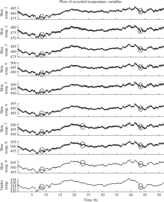
7.6.2 Description of sensor bias

Thermocouples for measuring skin temperatures are prone to measurement biases which usually recover after some hours. Should the temperature readings form part of a feedback control structure, it is necessary to detect such sensor faults as early as possible and to take appropriate action. During the recording period, several such events arose. Figure 7.17 shows one occurrence of a sensor bias in the thermocouple measuring Skin Temperature 5. It is important to note that the actual bias is just around 25°C. Comparing this with the range of temperature values in Figure 7.16, such a small bias can easily be overlooked by plant personnel. The next two subsections show the application of PCA and MWPCA to the normal operating data and the application of MWPCA to the data set describing the sensor bias.

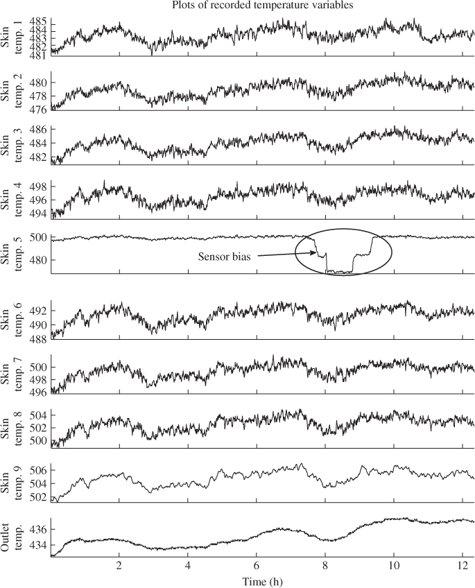
7.6.3 Application of PCA

To demonstrate that a fixed PCA model may run into difficulties if the mean and/or variance of the process variables changes significantly, this subsection applies a PCA monitoring model that is determined from the first half of the data and applied to the entire data set. The identification of a PCA model commenced by subtracting the mean of each variable and dividing it by the standard deviation, estimated from the samples in the first half of the data, and the estimation of the data correlation matrix. The eigendecomposition of the estimated covariance matrix then provided the required information to establish a PCA monitoring model.

The upper plot in Figure 7.18 shows the eigenvalues of the estimated data correlation matrix in descending order. The results of applying the VRE criterion is shown in the lower plot of Figure 7.18 and suggests three source signals. The control limits for the Hotelling's T² and Q statistics had to be determined. For α = 0.01, the control limits of the Hotelling's T² and Q statistics were 11.3684 and 0.2252, respectively.

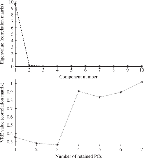
Figure 7.19 shows the performance of the PCA monitoring model over the entire data set. The Q statistic does not yield a significant number of violations. In contrast, the Hotelling's T² statistic presents a different picture. Whilst the first half shows few violations, there are massive violations in the second half of the data set. This is indicative of excessive common cause variation.

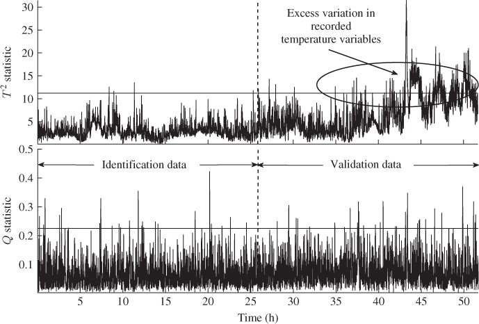
By comparing Figures 7.16 and 7.19, the last third of the data incorporates more variation in all of the temperature readings compared to the remaining data set, particulary the middle portion between 12 to 35 hours into the data set. Although the behavior of the furnace is not abnormal in the second half of the data, the fixed PCA model shows significant violations. This example, therefore, demonstrates that an adaptive model is needed in order adapt to the changes in variable mean, which is discussed in the next subsection.

7.6.4 Utilizing MWPCA based on an application delay

In order to establish a MWPCA model, the window size and the application delay need to be determined. Given that the number of variables is significantly smaller compared to the FCCU application study in Section 7.5, the window size may be made smaller. For a total of ten recorded process variables, Table 2.2 in Chiang et al. (2001) suggests that the minimum number of samples to populate the data covariance/correlation matrix is 118. Following the discussion in Subsection 7.3.6, this number does not take the high degrees of correlation into account.

Inspecting Figure 7.16 highlights that the ten temperature readings follow a very similar pattern and are, consequently, highly correlated, which the upper plot in Figure 7.18 confirms. More precisely, the last 7 eigenvalues are close to zero. Regarding the analysis in Subsection 7.3.6, given that these eigenvalues determine the control limit of the Q statistic, any significant estimation error would have a profound impact for determining Q_α, as the estimation error depends reciprocally on the window size. To ensure that the window size is significantly larger then the suggestion of 118, was selected to be 900.

The next step involved choosing a value of the application delay . As illustrated in Subsections 7.4.3 and 7.5.5, this delay can be determined empirically. The empirical significance for various values of was obtained for the reference data. Table 7.8 summarizes the results and outlines that significant increases of the empirical significance arise for values over 20 for the Hotelling's T² statistic and for values over 30 for the Q statistic. This suggests a selection of .

Table 7.8 Empirical significance

Application horizon
1	0.008107	0.003506
2	0.008764	0.004163
3	0.008326	0.004382
4	0.008326	0.004601
5	0.008326	0.004601
6	0.008545	0.004820
7	0.008545	0.004820
8	0.009202	0.005039
9	0.008764	0.006135
10	0.008983	0.006354
15	0.009422	0.006573
20	0.010955	0.007011
25	0.011394	0.008545
30	0.012489	0.011174
35	0.014461	0.014899
40	0.017528	0.017090
45	0.018843	0.017748
50	0.020377	0.019500

After selecting and , Figure 7.20 confirms that MWPCA model adapts this behavior. Moreover, the MWPCA monitoring model is still able to detect the erratic, abrupt and unsteady glitches, encircled in Figure 7.16. Samples corresponding to these short violations are removed from adapting the MWPCA model to ensure that no corruption of the monitoring model arises. Overall, the number of violations does not exceed the significance of 0.01, which implies that the reference data described the process in-statistical-control. It is also interesting to note that the number of source signals varies between one and four. Changes in this number, however, occur infrequently and three PCs are retained most of the time.

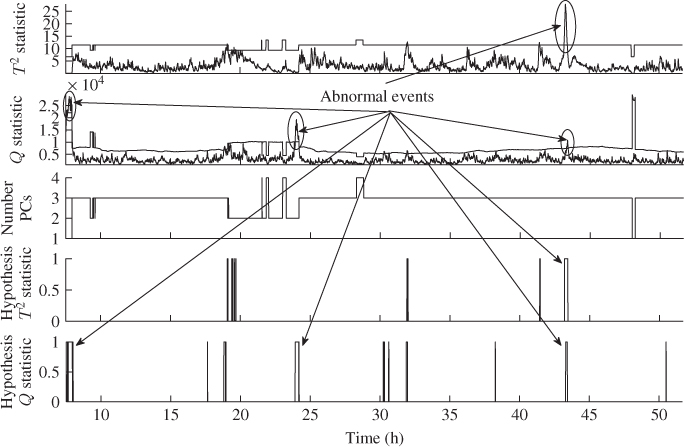
Finally, Figure 7.21 shows that the MWPCA model can detect the sensor bias in Skin Temperature 5. The Q statistic is sensitive to this event just after 7 hours and 37 minutes into the data set. The first 7 hours and 30 minutes of data cover the initial moving window Hence, the abscissa in Figures 7.20 and 7.21 does not start from zero. The Hotelling's T² statistic provided constant violations of its control limit starting from 7 hours and 40 minutes into the data. After detecting the sensor bias, the adaptation of the MWPCA model was suppressed.

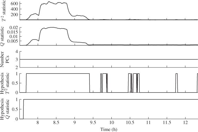
According to Figure 7.17, the sensor bias arose just after 7 hours and 35 minutes and remained up until 9 hours and 20 minutes into the data set. By comparison, the sensor fault could be detected almost instantly. The bottom two plots in Figure 7.21 highlight that the Hotelling's T² statistic violates the control limit from 9 hours and 25 minutes and thereafter with noticeable and sporadic violations just before 10 hours and after 10 hours and 30 minutes and after 11 hours and 40 minutes. In contrast, the Q statistic remains violating its control limit.

That the Hotelling's T² statistic does not show significant violations after 9 hours and 25 minutes implies that the three source signals showed a state of in-statistical control. However, the underlying geometry of the PCA model has changed compared to the now time-invariant model that was last updated before detecting the sensor bias. If a plant operator examines the situation at that point and determines that the sensor readings are correct, the adaptation of the MWPCA model can continue.

The analysis of both data sets, therefore, confirmed that the application MWPCA can adapt to changes in the variable mean and data correlation matrix and subsequently the PCA monitoring model. The adaptive monitoring model is also able to detect the sensor bias. To verify which of the sensors is faulty, contribution charts or variable reconstruction can be used as discussed in Subsection 3.2.1.

7.7 Adaptive partial least squares

In a similar fashion to PCA, the adaptation of a PLS model can be carried out on the basis of a recursive or a moving window formulation. The first step involves the adaptation of the estimated mean vectors for the input and output variables. This can be accomplished by applying (7.3) for the recursive and (7.21) for the moving window formulation by replacing the process with the input and output variables.

The next step is the adaptation of the covariance and cross-covariance matrices. For the reasons outlined in Jackson (2003) and Remark 7.2.1 above, it is advisable to scale the process variables to unity variance. The covariance and cross-covariance matrix consequently become the correlation and cross-correlation matrix. This entails the division of the input and output variable sets by the estimated standard deviation, which must be adapted too. Equations (7.4) and (7.22) show the recursive and moving window adaptation of the standard deviation, respectively.

This section first outlines how to adapt the correlation and cross-correlation matrices recursively and by applying a moving window formulation in Subsections 7.7.1 and 7.7.2, respectively. Subsection 7.7.3 then discusses how to adapt the number of source signals n and finally, Subsection 7.7.4 summarizes the adaptation of the PLS model. It should be noted that the adaptation of the control limits follows from the discussion in Subsection 7.3.4 and is therefore not covered in this section.

It is also advisable to consider the use of an application delay (Subsection 7.3.5) to improve the sensitivity in detecting incipient fault conditions. This follows from the benefits outlined by the simulation examples in Sections 7.4 and 7.5. Finally, another important aspect is the minimum size of the initial reference set (RPLS) or the size of the moving window (MWPLS). As outlined in Subsection 7.3.6, this is still an issue that has not been exhaustively studied and still requires further attention by the research community. As before, the notation to denote estimates of the weight vectors is omitted in this section to simplify the presentation of the equations.

7.7.1 Recursive adaptation of and

The adaptation of the correlation matrix of the input variables is identical to adaptation of for recursive PCA in Section 7.2. Including the (k + 1)th sample of the input variables, (7.62) shows the recursive update of to become

7.62

Here, , and are obtained in the same way as shown in (7.4) and (7.5) for the data vector z₀(k + 1).

The recursive adaptation of the cross-correlation matrix requires the adaptation of the mean and variance of both variable sets and is given by

7.63

Table 7.9 summarizes the steps for determining the auxiliary variables involved in (7.62) and (7.63) and the complete recursive adaptation of both matrices.

Table 7.9 Recursive adaptation of covariance and cross-covariance matrices

No.	Variables	Description
1		Adapt the mean vectors
2		Difference between consecutive mean vectors
3		Adapt diagonal matrix storing the standard deviations of the input variables
4		Adapt diagonal matrix storing the standard deviations of the output variables
5		Centering and scaling the new sample of the input and output variables
6		Recursive adaptation of and

7.7.2 Moving window adaptation of and

As shown in Section 7.3, the recursive adaptation of for and can be developed further to yield a moving window adaptation. This is based on the three-step procedure, which is outlined in Figure 7.1. By reformulating (7.7) to (7.23), Table 7.10 summarizes the steps involved in the moving window adaptation of and .

Table 7.10 Moving window adaptation of and .

Step	Equations	Description
1		Mean of Matrix II
2	,	Difference in mean vectors
3		Scale discarded sample for input and output variables
4		Bridge old and new data window
5		Mean of new data window
6	,	Mean vector difference
7		Standard deviations for variables in new data window
8		Storing standard deviations in diagonal scaling matrices
9		Scale input and output vector of new sample
10		Update of correlation and cross-correlation matrix

7.7.3 Adapting the number of source signals

Subsection 2.4.2 provides a list of stopping rules to determine the number of source signals. From these, techniques that rely on reference sets, such as cross validation or bootstrapping methods may not suitable, given that the relationship among and between the input and output variables are assumed to be time varying.

An alternative is to evaluate the accuracy of predicting the output variables. Equation (2.147) shows how to describe the accuracy in terms of the PRESS statistic for the initial model. With a new sample becoming available, the accuracy for predicting the output variables of this sample can be determined and compared with the prediction accuracy of the initial model.

For a moving window formulation, the selection of n is then as follows

7.64

where is the resultant PRESS statistic of the th sample for the retention of n sets of LVs, and are updated matrices, k + 1 referring to the new sample, storing the first n_k+1 -loading and r-weight vectors, respectively, and describes the accuracy of the initial PLS model, retaining the initial selection of n₁ sets of LVs. The next subsection describes the complete adaptation procedure for a PLS model.

7.7.4 Adaptation of the PLS model

As for adaptive PCA models, the number of source signals may vary over time, resulting from throughput, grade changes or operator interventions that may yield short-term transients behavior between different operating conditions for example. On the other hand, the difference between the initial and adapted weight vectors, that is, , is expected to be small. This implies that the iterative PLS routine converges after the first few iteration steps for each set of LVs unless significant change in the process behavior has arisen.

To maintain this efficiency for a varying number of source signals, it is possible to employ the approach introduced in Subsection 7.3.2. This entails the storage and adaptation of a number of sets of weight vectors that is larger than n_k. If n_k+1 > n_k, this this approach ensures that more sets of LVs are available to test whether . The number of pairs of weight vectors that are temporarily stored are n_k + 1 + j, where j is an integer that is also adaptively computed. The following list of steps summarizes the adaptive PLS algorithm, based on the steps discussed above:

7.8 Tutorial Session

Question 1:

Explain how window size affects the accuracy of the adapted model and how does it affect the detectability of faults? Summarize and comment upon the recommendations in the existing work on determining the window length.

Question 2:

What are the advantages and disadvantages of using a recursive and a moving window adaptation of PCA and PLS models?

Question 3:

What is the reason behind the introduction of an application delay?

Question 4:

What are the steps for adapting a PCA- and PLS-based monitoring model?

Project:

Using a Monte Carlo simulation on the basis of the example in (7.37) to (7.40), determine the effect of a varying window length , a varying application horizon and a varying slope for the ramp describing time-varying process behavior upon the empirical significance level. If the ramp is considered as a fault condition, how does the window length and the application horizon affect the average run length?

 

 

¹ To be more precise, the unit of the elements of the correlation matrix is 1.