Chapter 9
Principal component analysis
This chapter introduces the PCA algorithm, including a discussion showing that the computed score and loading vectors maximize their contribution to the column and row space of a data matrix. A summary of PCA and the introduction of a preliminary PCA algorithm then follows in Section 9.2. A detailed summary of the properties of PCA is given in Section 9.3. Without attempting to give a complete review of the available research literature, further material concerning PCA may be found in Dunteman (1989); Jackson (2003); Jolliffe (1986); Wold (1978); Chapter 8 in Mardia et al. (1979) and Chapter 11 in Anderson (2003).
9.1 The core algorithm
PCA extracts sets of latent variables from a given data matrix  , containing K mean-centered and appropriately scaled samples of a variable set
9.1 
The scaling matrix  is a diagonal matrix and often contains the reciprocal values of the estimated standard deviation of the recorded variables
9.2 
Based on  , PCA determines a series of rank-one matrices
9.3 
constructed from the estimated score and loading vectors,  and
and  , respectively. After extracting a total of n such rank one matrices, the residual matrix is
  . According to the non-causal data structure in (2.2), for which a detailed discussion is available in Section 6.1, an estimate of the column space of the parameter matrix Ξ is given by the loading matrix, i.e.
  . As outlined in Section 6.1 the residual matrix is equal to the matrix product of Z0 and an orthogonal complement of
  , which spans the residual subspace. The construction of the model subspace, that is, the estimation of the column vectors of
  , and the residual subspace using PCA is now discussed. For simplicity, the subscript j is omitted for outlining the PCA algorithm.
Capturing the maximum amount of information from the data matrix Z0, each rank one matrix relies on a constraint objective function. Pre-multiplying Z0 by  allows extracting information from its column space
9.4 
Post-multiplying Z0 by  allows extracting information from its row space
9.5 
The two equations above give rise to the following objective functions
9.6a 
9.6b 
which are subject to the constraints
9.7a 
9.7b 
In the above equations,  and
and  are, up to a scalar factor, covariance matrices of the column space and the row space of Z0, respectively. Both matrices are symmetric and, assuming that z can be constructed from the data structure in (2.2), Mpp and Mττ being positive definite and positive semi-definite, respectively, if K
  nz. Moreover,
  is a scaled variance measure and
  is a sum of squares measure for the column and row space of Z0, respectively.
The solutions to the constraint objective functions in (9.6a) are given by
9.8a 
9.8b 
where μp and μτ are Lagrangian multipliers. Substituting the definition of Jp, Jτ, Cp and Cτ in (9.6a) and carrying out the above relationships gives rise to
9.9a 
9.9b 
Equation (9.9a) implies that
9.10a 
9.10b 
and hence,
9.11a 
9.11b 
Lemma 9.1.1
The Lagrangian multipliers μp and μτ are larger than zero, identical and are equal to the estimated variance of the jth largest principal component, 1 ≤ j ≤ n, if K  nz.
nz.
Proof.
That μ
p and μ
τ are larger than zero follows from the objective functions in (
9.6a)
9.12a 
9.12b 
Given that

and
Z0 ≠
0, it follows that

and

. To proof that
Jp = J
τ and hence, μ
p = μ
τ, consider a singular value decomposition of

, where the matrices

and

contain the left and right singular vectors, respectively, and

is a diagonal matrix storing the singular values in descending order, which yields
9.13a 
9.13b 
where

. Since the matrix expressions

and

represent the eigendecomposition of
Mpp and
Mττ, respectively, it follows that the eigenvalues of
Mpp and
Mττ are identical and equal to the diagonal elements of
Λ. Using
- the fact that
 and
and  , which results from (9.9a) to (9.11a);
- the fact that
 and
and  are the dominant eigenvectors of Mpp and Mττ, respectively; and
- a reintroduction of the subscript j,
it follows that
9.14 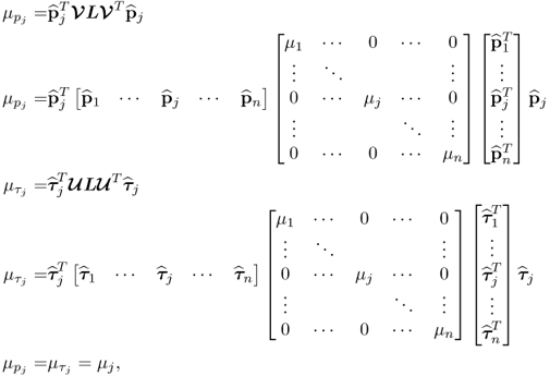
since the eigenvectors are mutually orthonormal.
Finally, to prove that μj is equal to the contribution of the jth component matrix to the data matrix Z0 relies on post- and pre-multiplying the relationships in (9.9a) by  and
and  , which yields
9.15 
Equation (9.15) can be further simplified by defining  ,
,  ,
,  and
and  , since
9.16 
The contribution of the jth rank-one component matrix to the data matrix Z0 is equal to the squared Frobenius norm of 
9.17 
Theorem 9.1.2
If the covariance matrix
9.18 
where
9.19 
is used in the above analysis, the variance of the jth t-score variable is equal to the Lagrangian multiplier λj, that is, the jth largest largest eigenvalue of  .
.
Proof.
The variance of the score variable
tj,

is given by
9.20 
On the basis of the objective functions in (9.6a) and the constraints in (9.7a), the first rank-one component matrix,  , has the most significant contribution to Z0. This follows from
  , which, according to (9.9a) and (9.9b), is the most dominant eigenvector of Mpp and the fact that
  , which follows from (9.16). It should also be noted that μj = (K − 1)λj when the estimate of
  is or used.
After subtracting or deflating the rank-one matrix  from Z0, that is
  with Z(1) = Z0, the rank-one matrix
  has the most significant contribution to Z(2). Moreover,
  and
and  is the most dominant eigenvector of
  ,
,
9.21 
Utilizing the deflation procedure, the first n eigenvalues and eigenvectors of  can be obtained using the Power method (Geladi and Kowalski 1986; Golub and van Loan 1996). Alternatively, a PCA model can also be determined by a singular value or eigendecomposition of
  , which is computationally more economic (Wold 1978). Based on the covariance matrix, it should also be noted that the objective function for determining the ith loading vector can be formulated as follows
9.22 
9.2 Summary of the PCA algorithm
The above analysis showed that PCA determines linear combinations of the variable set z0 such that the variance for each linear combination is maximized. The variance contribution from each set of linear combinations is then subtracted from z0 before determining the next set. This gives rise to a total of nz combinations that are referred to as score variables. Combining the parameters for each of the linear combinations into a vector yields loading vectors that are of unit length. If the covariance matrix of the data vector z0, i.e.  is available, and the data vector follows the data structure
  , where
  ,
,  ,
,  ,
,  and
and  for all 1 ≤ j ≤ nz, the following holds true:
- the largest n eigenvalues of
 are larger than
  and represent the variance of the dominant score variables, that is, the retained score variables;
- the remaining nz − n eigenvalues are equal to
 and describe the variance of the residuals, that is, the discarded score variables; and
- the first n eigenvectors allow one to extract linear combinations that describe the source signals superimposed by some error vector.
The above properties are relevant and important for process monitoring and are covered in more detail in Subsections 1.2.3, 1.2.4, 3.1.1, 3.1.2 and 6.1.1. In essence, the eigendecomposition of  contains all relevant information to establish a process monitoring model. Table 9.1 summarizes the steps for iteratively computing the eigendecomposition of
  using the deflation procedure in (9.21). It should be noted, however, that the eigenvalues and eigenvectors of
  can also be obtained simultaneously without a deflation procedure, which is computationally and numerically favorable over the iterative computation. The algorithm in Table 9.1 is based on the covariance matrix
  .
.
Table 9.1 Iterative PCA algorithm
| 1 |
Initiate iteration |
j = 1 |
| 2 |
Obtain initial matrix |
 |
| 3 |
Set-up initial loading vector |
 |
| 4 |
Calculate matrix-vector product |
 |
| 5 |
Compute eigenvalue |
 |
| 6 |
Scale eigenvector |
 |
|
|
If ||1pj − 0pj|| > ε , set |
| 7 |
Check for convergence |
0pj = 1pj and go to Step 4 else |
|
|
set pj = 1pj and go to Step 8 |
| 8 |
Deflate matrix |
 |
|
|
If j < nz set j = j + 1 |
| 9 |
Check for dimension |
and go to Step 3 else |
|
|
terminate iteration procedure |
9.3 Properties of a PCA model
The PCA algorithm has the following properties:
1. Each rank-one component matrix produces a maximum variance contribution to the data matrix
Z0 in successive order, that is,

produces the largest,

the second largest and so on.
2. The t-score vectors are mutually orthogonal.
3. The p-loading vectors are mutually orthonormal.
4. Under the assumption that the source variables are statistically independent, the t-score variables follow asymptotically a Gaussian distribution.
5. It is irrelevant whether the score vector

is computed as the matrix vector product of the original data matrix,
Z0, or the deflated data matrix,
Z(j), and the loading vector

.
6. If that the rank of
Z0 is
 z
z ≤
nz,
Z0 is completely exhausted after
 z
z deflation procedures have been carried out.
7. The data covariance matrix

can be reconstructed by a sum of
 z
z scaled loading vectors
pj.
These properties are now mathematically formulated and proven. Apart from Properties 4 and 7, the proofs rely on the data matrix Z0 and estimates of the score and loading vectors. Properties 4 and 7 are based on a known, that is, not estimated, data structure  and covariance matrix
  , respectively.
Property 9.3.1 – Contribution of Score Vectors to Z0.
The contribution of each score vector to the recorded data matrix is expressed by the rank-one component matrices

. Theorem 9.3.1 formulates the contribution of each of these component matrices to recorded data matrix.
Theorem 9.3.1
In subsequent order, the contribution of each rank-one component matrix,  , is maximized using the PCA algorithm.
Proof.
Knowing that the process variables are mean-centered, the sum of variances of each process variable,

, is equal to the squared Frobenius norm of
Z0 up to a scaling factor. Moreover, the eigendecomposition of

describes, in fact, a rotation of the
nz dimensional Euclidian base vectors to be the eigenvectors of

. Under the assumption that

has full rank
nz, this implies that (
9.3) can be rewritten as follows
9.23 
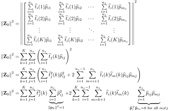
The next step involves working out the Frobenius norm of (
9.23), which gives rise to
9.24 
Simplifying (
9.24) by determining the sum of the squared elements of
Z0 yields
9.25 
and hence
9.26 
The Lagrangian multiplier μ
j, however, represents the maximum of the objective functions

and

. Hence, the variance contribution of

to
Z0 is the
jth largest possible. That

for all i ≠ j follows from the fact that the eigenvectors of
Mpp are mutually orthonormal and hence,

. Moreover, Theorem 9.1.2 outlines that the
jth largest eigenvalue of the data covariance matrix

is equal to the variance of the
jth score variable

.
Property 9.3.2 – Orthogonality of the t-Score Vectors.
Next, examining the deflation procedure allows showing that the t-score vectors are mutually orthogonal. It should be noted, however, that the orthogonality properties of these vectors also follow from the t-score vectors are dominant eigenvectors of the symmetric and positive semi-definite matrix Mττ, respectively. Theorem 9.3.2 formulates the orthogonality of the t-score vectors.
Theorem 9.3.2
The deflation procedure produces orthogonal t-score vectors, that is, 
,

,

.
Proof.
The expression

can alternatively be written as

, which follows from (
9.16). Without restriction of generality, assuming that
i >
j the deflation procedure to reconstruct
Z(i) gives rise to
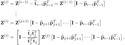
9.27 
Substituting (
9.27) into

produces
9.28 
and hence
9.29 
Consequently,

Property 9.3.3 – Orthogonality of the p-Loading Vectors.
The deflation procedure also allows showing mutual orthogonality of the p-loading vectors, which is discussed in Theorem 9.3.3. It is important to note that the orthogonality of the p-loading vectors also follows from the fact that they are eigenvectors of the symmetric and positive definite matrix Mpp.
Theorem 9.3.3
The deflation procedure produces orthonormal p-loading vectors, i.e. 
.
Proof.
The proof commences by rewriting

. Reformulating the deflation procedure for
Z(i)9.30 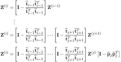
and substituting this matrix expression into

yields
9.31 
Thus,

Property 9.3.4 – Asymptotic Distribution of t-Score Variables.
It is expected that for a large numbers of source variables the score variables are approximately Gaussian distributed. A more precise statement to this effect is given by the Liapounoff theorem. A proof of this theorem, in the context of the PCA score variables, relies on the data structure

for the error covariance matrix

. This data structure guarantees that the covariance matrix

has full rank
nz. Moreover,

has the following eigendecomposition
PΛPT, where the loading vectors
p1, …,

are stored as column vectors in
P and the diagonal matrix
Λ stores the variances of the score variables λ
1, …, λ
n and a total of
nz −
n times the variance of the error variables

.
Theorem 9.3.4
For the data structure  ,
,  ,
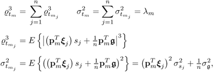
,  and the assumption that the source variables s are independently but not identically distributed with unknown distribution functions, the score variables are approximately Gaussian distributed if n is sufficiently large and none of the individual source variables have a significant influence on the determination of the score variables, which can be expressed by the following condition (Liapounoff 1900, 1901)
9.32 
where
9.33 
and  is the variance of the jth source variable.
Proof.
In the context of the t-score variables for PCA, obtained as follows
9.34 
the Liapounoff theorem outlines that if
n is sufficiently large and none of the sum elements

is significantly larger than the remaining ones, the score variables are asymptotically Gaussian distributed as n → ∞. A proof for the case where the distribution function of the
n sum elements

are i.i.d. is given in Subsection 8.7.1 under a simplified version of the Lindeberg-Lévy theorem. The presented proof of Theorem 9.3.4 assumes that these elements are only i.d. and meet the condition outlined in (
9.31) and (
9.33).
It should be noted, however, that the CLT holds true for more general conditions than that postulated by Liapounoff (1900, 1901). A detailed discussion of more general conditions for the CLT may be found in Billingsley (1995); Bradley (2007); Cramér (1946); Durrett (1996); Feller (1936, 1937); Fisher (2011) and Gut (2005) for example. More precisely, the assumption of statistically independent source signals can be replaced by mixing conditions (Bradley 2007). An exhaustive treatment of mixing conditions, however, is beyond the scope of this book and the utilization of the Liapounoff theorem, imposing statistical independence upon the source signals, serves as an extension to the i.i.d. assumptions associated with the Lindeberg-Lévy theorem. Interested readers can resort to the cited literature above for a more general treatment of the CLT.
Assuming that the random variables

have the distribution functions
F1(
s1),
F2(
s2), …,
Fn(
sn), the proof of Theorem 9.3.4 relies on the characteristic function of

, which is defined as
9.35 
where

and the scaled score variables τ
m has zero mean, unity variance and the distribution function
F(
s). As n → ∞ the term

and can, consequently, be omitted. Next, substituting (
9.34) into the definition of the characteristic function of τ
m yields
9.36 
The remaining elements of the sum,

, are i.d. according to the assumptions made in Theorem 9.3.4. Hence, (
9.36) can be rewritten as follows
9.37 
If
9.38 
the term

is Gaussian distributed, as

is the characteristic function of a zero mean Gaussian distribution of unity variance. Approximating the expression for the product terms γ
j(
c) by a Taylor series expansion, developed around
c = 0, shows that

as n → ∞
9.39 
Here, 0 ≤ τ ≤ c and

is the remainder in Lagrangian form. The relationships

, are given by
9.40 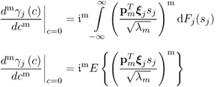
and yields:
and for the Lagrangian remainder

Here, |ϑ| < 1 is a complex constant. Thus, the Taylor series in (
9.39) reduces to
9.41 
where

. Recall that (
9.41) expresses the
jth terms of

. Rewriting this equation in logarithmic form allows transforming the product into a sum, since
9.42 
which simplifies the remainder of this proof. Equation (
9.43) gives the logarithmic form of (
9.41)
9.43 
Here,

. For a sufficiently large number of source signals
n, it follows from (
9.32) and (
9.33) that
9.44 
Equation (
9.45) presents a different way to formulate
z9.45 
Here,

is a small correction term. Equations (
9.32), Equations (
9.44) and (
9.45) highlight that
9.46 
as

. This implies that if the number of source signals
n is large enough, |
z| < 0.5, which, in turn, allows utilizing the Taylor expansion for log(1 +
z) to produce
9.47 
where

is, as before, a small correction term. Hence,
9.48 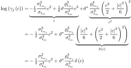
with ϑ
* being, again, a small correction term. For

being another small correction term, the final step is summing the individual terms, γ
j(
c), according to (
9.42), which yields
9.49 
According to (
9.32) and (
9.33), (
9.49) becomes
9.50 
and hence
9.51 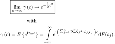
Consequently, the mth t-score variable asymptotically follows a Gaussian distribution under the assumption that the source signals are statistically independent. As stated above, however, the conditions for which the CLT holds true are less restrictive than those formulated in the Liapounoff and the simplified Lindeberg-Lévy theorems used in this book. The interested reader can refer to the references given in this proof for a more comprehensive treatment of conditions under which the CLT holds true.
Property 9.3.5 – Computation of the t-Score Vectors.
After proving the asymptotic properties of the t-score variables with respect to the number of source variables, the impact of the deflation procedure upon the computation of the t-score vectors is analyzed next.
Theorem 9.3.5
It is irrelevant whether the jth t-score vector  are obtained from the original or the deflated data matrix, that is,
  .
.
Proof.
Starting with Z(j)pj and revisiting the deflation of Z(j)
9.52 
which yields
9.53 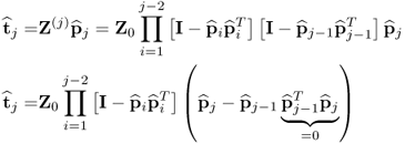
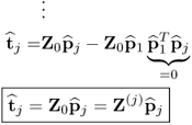
That the p-loading vectors are mutually orthonormal is subject of Theorem 9.3.3.
Property 9.3.6 – Exhausting the Data Matrix Z0.
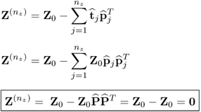
The deflation procedure allows exhausting the data matrix if enough latent components are extracted.
Proof.
It is straightforward to prove the case
 z
z =
nz, which is shown first. The general case
 z
z <
nz is then analyzed by a geometric reconstruction of
Z0 using the rank-one component matrices shown in (
9.3). If
 z
z =
nz the following holds true
9.54 
which follows from the fact that (i) the estimated p-loading vectors are orthonormal and (ii) that

.
In the general case where
 z
z <
nz, the observations stored as row vectors in
Z0 lie in a subspace of dimension
 z
z. This follows from the fact that any
nz −
 z
z column vectors of
Z0 are linear combinations of the remaining
 z
z columns. We can therefore remove
nz −
 z
z columns from
Z0, which yields a reduced dimensional data matrix

. According to (
9.54),

is exhausted after
 z
z deflation steps have been carried out. Given that the columns that were removed from
Z0 are linear combinations of those that remained in

, deflating the reduced data matrix

automatically deflates the column vectors not included in

.
Property 9.3.7 – Exhausting the Covariance Matrix  .
.
The final property is concerned with the reconstruction of the given covariance matrix

using the loading vectors
p1, …,

, where
 z
z ≤
nz is the rank of

. Whilst this is a property that simply follows from the eigendecomposition of a symmetric positive semi-definite matrix, its analysis is useful in providing an insight into the deflation procedure of the PLS algorithm, discussed in Section 10.1.
Lemma 9.3.7
The covariance matrix  can be reconstructed by a sum of
  z ≤ nz scaled loading vectors pj, where the scaling factor is given by the standard deviation of the score variables.
Proof.
A reformulation of (
9.6a) leads to
9.55 
and hence
9.56 
Given that the rank of

, there are a total of
 z
z eigenvalues λ
j that are larger than zero. Equation (
9.56) can be expanded to allow a simultaneous determination of the
 z
z eigenvectors
9.57 
which follows from the fact that the eigenvectors are mutually orthonormal (Theorem 9.3.3) and that

(Theorem 9.3.6). The optimum of the individual objective functions, combined in (
9.57), is given by
9.58 
which gives rise to
9.59 
Substituting the fact that

, pre-multiplication of the above equation by
PT yields
9.60 
which represents the diagonalization of

. On the other hand, the relationship above also implies that
9.61 
and hence
9.62 
It should be noted that (
9.61) holds true since
PPT projects any vector onto the subspace describing the relationship between any
nz −
 z
z variables that are linearly dependent upon the remaining
 z
z ones. This subspace is spanned by the
 z
z eigenvectors stored in
P.
Note that the column vectors of  and
and  are orthonormal and are the eigenvectors of Mpp and Mττ, respectively (Golub and van Loan 1996).
A dominant eigenvector is the eigenvector that corresponds to the largest eigenvalue of a given squared matrix.
Note that the relationship below takes advantage of the fact that  , which follows from (9.15) and (9.16)
The assumption of  is imposed for convenience and does not represent a restriction of generality as the following steps are also applicable for
  .
.
![]() , containing K mean-centered and appropriately scaled samples of a variable set
, containing K mean-centered and appropriately scaled samples of a variable set ![]()
![]()
![]() is a diagonal matrix and often contains the reciprocal values of the estimated standard deviation of the recorded variables
is a diagonal matrix and often contains the reciprocal values of the estimated standard deviation of the recorded variables
![]() , PCA determines a series of rank-one matrices
, PCA determines a series of rank-one matrices![]() and
and ![]() , respectively. After extracting a total of n such rank one matrices, the residual matrix is
, respectively. After extracting a total of n such rank one matrices, the residual matrix is ![]() . According to the non-causal data structure in (2.2), for which a detailed discussion is available in Section 6.1, an estimate of the column space of the parameter matrix Ξ is given by the loading matrix, i.e.
. According to the non-causal data structure in (2.2), for which a detailed discussion is available in Section 6.1, an estimate of the column space of the parameter matrix Ξ is given by the loading matrix, i.e. ![]() . As outlined in Section 6.1 the residual matrix is equal to the matrix product of Z0 and an orthogonal complement of
. As outlined in Section 6.1 the residual matrix is equal to the matrix product of Z0 and an orthogonal complement of ![]() , which spans the residual subspace. The construction of the model subspace, that is, the estimation of the column vectors of
, which spans the residual subspace. The construction of the model subspace, that is, the estimation of the column vectors of ![]() , and the residual subspace using PCA is now discussed. For simplicity, the subscript j is omitted for outlining the PCA algorithm.
, and the residual subspace using PCA is now discussed. For simplicity, the subscript j is omitted for outlining the PCA algorithm.![]() allows extracting information from its column space
allows extracting information from its column space![]()
![]() allows extracting information from its row space
allows extracting information from its row space![]()
![]()
![]()
![]() and
and ![]() are, up to a scalar factor, covariance matrices of the column space and the row space of Z0, respectively. Both matrices are symmetric and, assuming that z can be constructed from the data structure in (2.2), Mpp and Mττ being positive definite and positive semi-definite, respectively, if K
are, up to a scalar factor, covariance matrices of the column space and the row space of Z0, respectively. Both matrices are symmetric and, assuming that z can be constructed from the data structure in (2.2), Mpp and Mττ being positive definite and positive semi-definite, respectively, if K ![]() nz. Moreover,
nz. Moreover, ![]() is a scaled variance measure and
is a scaled variance measure and ![]() is a sum of squares measure for the column and row space of Z0, respectively.
is a sum of squares measure for the column and row space of Z0, respectively.![]()
![]()
![]()
![]()
![]()
![]()
![]()
![]()
![]()
![]()
 and
and  , which results from (9.9a) to (9.11a);
 and
and  are the dominant eigenvectors2 of Mpp and Mττ, respectively; and
![]() and
and ![]() , which yields
, which yields![]() ,
, ![]() ,
, ![]() and
and ![]() , since
, since![]()


![]()
![]() , has the most significant contribution to Z0. This follows from
, has the most significant contribution to Z0. This follows from ![]() , which, according to (9.9a) and (9.9b), is the most dominant eigenvector of Mpp and the fact that
, which, according to (9.9a) and (9.9b), is the most dominant eigenvector of Mpp and the fact that ![]() , which follows from (9.16). It should also be noted that μj = (K − 1)λj when the estimate of
, which follows from (9.16). It should also be noted that μj = (K − 1)λj when the estimate of ![]() is or used.
is or used.![]() from Z0, that is
from Z0, that is ![]() with Z(1) = Z0, the rank-one matrix
with Z(1) = Z0, the rank-one matrix ![]() has the most significant contribution to Z(2). Moreover,
has the most significant contribution to Z(2). Moreover, ![]() and
and ![]() is the most dominant eigenvector of
is the most dominant eigenvector of ![]() ,
,![]() can be obtained using the Power method (Geladi and Kowalski 1986; Golub and van Loan 1996). Alternatively, a PCA model can also be determined by a singular value or eigendecomposition of
can be obtained using the Power method (Geladi and Kowalski 1986; Golub and van Loan 1996). Alternatively, a PCA model can also be determined by a singular value or eigendecomposition of ![]() , which is computationally more economic (Wold 1978). Based on the covariance matrix, it should also be noted that the objective function for determining the ith loading vector can be formulated as follows
, which is computationally more economic (Wold 1978). Based on the covariance matrix, it should also be noted that the objective function for determining the ith loading vector can be formulated as follows![]()
![]() is available, and the data vector follows the data structure
is available, and the data vector follows the data structure ![]() , where
, where ![]() ,
, ![]() ,
, ![]() ,
, ![]() and
and ![]() for all 1 ≤ j ≤ nz, the following holds true:
for all 1 ≤ j ≤ nz, the following holds true: are larger than
  and represent the variance of the dominant score variables, that is, the retained score variables;
 and describe the variance of the residuals, that is, the discarded score variables; and
![]() contains all relevant information to establish a process monitoring model. Table 9.1 summarizes the steps for iteratively computing the eigendecomposition of
contains all relevant information to establish a process monitoring model. Table 9.1 summarizes the steps for iteratively computing the eigendecomposition of ![]() using the deflation procedure in (9.21). It should be noted, however, that the eigenvalues and eigenvectors of
using the deflation procedure in (9.21). It should be noted, however, that the eigenvalues and eigenvectors of ![]() can also be obtained simultaneously without a deflation procedure, which is computationally and numerically favorable over the iterative computation. The algorithm in Table 9.1 is based on the covariance matrix
can also be obtained simultaneously without a deflation procedure, which is computationally and numerically favorable over the iterative computation. The algorithm in Table 9.1 is based on the covariance matrix ![]() .
.![]() and covariance matrix
and covariance matrix ![]() , respectively.
, respectively.


![]()

![]()

![]()


 ;
; ; and
; and

![]()
![]()


![]()


![]() and
and ![]() are orthonormal and are the eigenvectors of Mpp and Mττ, respectively (Golub and van Loan 1996).
are orthonormal and are the eigenvectors of Mpp and Mττ, respectively (Golub and van Loan 1996).![]() , which follows from (9.15) and (9.16)
, which follows from (9.15) and (9.16)![]() is imposed for convenience and does not represent a restriction of generality as the following steps are also applicable for
is imposed for convenience and does not represent a restriction of generality as the following steps are also applicable for ![]() .
.


