Chapter 10
Partial least squares
This chapter provides a detailed analysis of PLS and its maximum redundancy formulation. The data models including the underlying assumptions for obtaining a PLS and a MRPLS model are outlined in Sections 2.2 and 2.3, respectively.
Section 10.1 presents preliminaries of projecting the recorded samples of the input variables,  onto an n-dimensional subspace, n ≤ nx, and show how a sequence of rank-one matrices extract variation from the sets of input and output variables x0 and
  , respectively. Section 10.2 then develops a PLS algorithm and Section 10.3 summarizes the basic steps of this algorithm.
Section 10.4 then analyzes the statistical and geometric properties of PLS and finally, Section 10.5 discusses the properties of MRPLS. Further material covering the development and analysis of PLS may be found in de Jong (1993); Geladi and Kowalski (1986); Höskuldsson (1988, 1996); ter Braak and de Jong (1998); Wold et al. (1984) and Young (1994).
10.1 Preliminaries
In a similar fashion to PCA, PLS extracts information from the input and output data matrices,  and
and  by defining a series of rank-one matrices
10.1a 
10.1b 
The data matrices store mean-centered observations of the input and output variable sets, that is  and
and  with
with  and
and  being mean vectors. In the above equation,
  and
and  are the rank-one matrices for the input and output matrices, respectively, the n vectors
  are t-score vectors which are estimated from the input matrix,
  and
and  are estimated loading vectors for the input and output matrices, respectively, and
  and
and  are residual matrices of the input and output matrices, respectively. It should be noted that the residual matrices have a negligible or no contribution to the prediction of the output data matrix.
To establish (10.1a), the PLS algorithm determines a sequence of parallel projections, one sequence for the observations stored in the input matrix and a second sequence for the observations stored in the output matrix. Reformulating (10.1a)
10.2a 
10.2b 
and defining
10.3a 
10.3b 
allows determining the sequence of projections for the input and output variables
10.4a 
10.4b 
Here,  is the u-score vector of the output matrix, and
  and
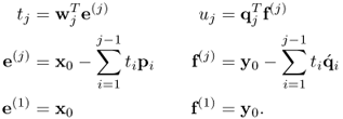
and  are the weight vectors for the input and output variable sets, respectively. Finally, according to (10.4a), the score variables, tk and uk, are given by
10.5 
The set of weight and loading vectors, wj, qj, pj and  , as well as the set of score variables, tj and uj, make up the jth latent variable set.
10.2 The core algorithm
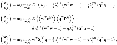
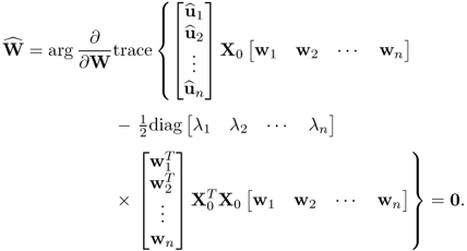
PLS determines the score variables tj and uj such that they maximize an objective function describing their covariance, which is subject to the constraint that the projection vectors wj and qj are of unit length
10.6 
where  . The optimal solution for the objective function in (10.6) is given by
10.7 
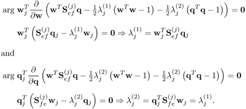
which have to be solved simultaneously. This yields
10.8 
Note that  . Equation (10.8) also confirms that the two Lagrangian multipliers are identical, since
10.9 
Hence,  . Combining the two expressions in (10.8) gives rise to
10.10a 
10.10b 
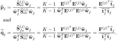
The weight vectors wj and qj are therefore the dominant eigenvectors of the matrix expressions  and
and  , respectively. The score vectors for E(j) and F(j) can now be computed using (10.4a).
After determining the weight and score vectors, the next step involves the calculation of a regression coefficient between the score variables tj and uj. It is important to note, however, that the determination of this regression coefficient can be omitted, as this step can be incorporated into the calculation of the  -loading vector, which is proven in Section 10.4. For a better understanding of the geometry of the PLS algorithm, however, the introduction of the PLS algorithm here includes this step. Equation (10.11) shows the least squares solution for determining the regression parameter
10.11 
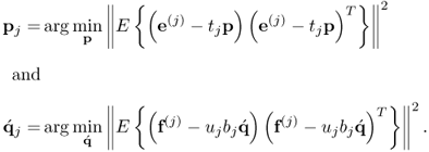
where  . The final step to complete the determination of the jth set of latent variables requires formulation of objective functions for computing the loading vectors
10.12 
The solutions to (10.12) are
10.13 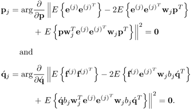
Working out the relationships yields
10.14 
Before computing the (j + 1)th set of LVs, (10.5) highlights that the contribution of the jth set of latent variables must be subtracted from e(j) and f(j)
10.15a 
10.15b 
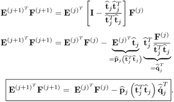
It should be noted that substituting (10.14) into (10.15a) gives rise to
10.16 
which, however, requires the  -loading vector to be determined as follows
10.17 
It should also be noted that the deflation procedure can be applied directly to the covariance matrix  and the cross-covariance matrix
10.18 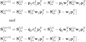
The above relationship relies on (10.14), (10.15a) and (10.17).
The steps of the PLS algorithm can be carried out using the NIPALS algorithm (Geladi and Kowalski 1986), the SIMPLS algorithm (de Jong 1993) or the computationally more efficient Kernel algorithms (Dayal and MacGregor 1997a; Lindgren et al. 1993; Rännar et al. 1994). Each of these algorithms are iterative in nature, that is, one pair of latent variables are obtained and the contribution of the t-score vector is deflated from the input and output matrices in one iteration step.
10.3 Summary of the PLS algorithm
The preceding analysis showed that PLS extracts covariance information from the input and output variables, x0 and y0, by defining a sequence of score variables which are extracted from the input variable set (10.5). The contribution of each score variable is maximized by the determination of loading vectors, such that the original variable sets are defined by  and
and  (10.15).
The calculation of the n score variables, t1, t2, …, tn relies on an objective function that maximizes a covariance criterion between ti and a score variable that is extracted from the output variable set ui, E{tiui} (10.6). In other words, there are a total of n score variables computed from the input variable set and n score variables calculated from the output variable set. These score variables are obtained in pairs, ti and ui and are given by a projection of the input and output variable set onto the weight vectors wi and qi (10.5). The solution for the pairs of weight vectors gives rise to the determination of dominant eigenvectors of symmetric and positive semi-definite matrices.
Unlike the PCA algorithm, the sets of latent variables can only be determined sequentially using the power method (Geladi and Kowalski 1986). This is an iterative method for determining the dominant eigenvector of a symmetric positive semi-definite matrix (Golub and van Loan 1996). Using the basic steps, developed in the previous subsection, Table 10.1 presents a PLS algorithm for determining the weight and loading vectors from the covariance matrix  and the cross-covariance matrix
  . The next subsection presents a detailed statistical and geometric analysis of the PLS algorithm and introduces a computationally more efficient algorithm to that described in Table 10.1.
Table 10.1 PLS algorithm developed from the steps in Section 10.2.
| 1 |
Initiate iteration |
j = 1 |
| 2 |
Obtain covariance matrix |
 |
| 3 |
Determine cross-covariance matrix |
 |
| 4 |
Set-up initial q-weight vector |
 |
| 5 |
Calculate w-weight vector |
 |
| 6 |
Scale w-weight vector to unit length |
 |
| 7 |
Compute q-weight vector |
 |
| 8 |
Scale q-weight vector to unit length |
 |
|
|
If ||1qj − 0qj|| > ϵ, set |
| 9 |
Check for convergence |
0qj = 1qj and go to Step 5; else go to Step 10 |
| 10 |
Determine p-loading vector |
 |
| 11 |
Calculate  -loading vector -loading vector |
 |
| 12 |
Deflate cross-covariance matrix |
 |
|
Check whether there is significant |
If so, go to Step 14 |
| 13 |
variation left in the cross- |
if not, terminate modeling |
|
covariance matrix |
procedure |
| 14 |
Deflate covariance matrix |
 |
|
|
If j < nx, set j = j + 1 |
| 15 |
Check for dimension |
and go to Step 4 |
|
|
if not, terminate modeling |
|
|
procedure |
10.4 Properties of PLS
The PLS algorithm, developed and summarized in the last two subsections, has the statistical and geometrical properties listed below. For a detailed discussion of these properties, it is important to note that the preceding discussion has assumed the availability of the covariance matrix  and the cross-covariance matrix
  . This has been for the convenience and simplicity of the presentation. Unless stated otherwise, the analysis that follows, however, removes this assumption and relies on the available data matrices X0 and Y0, whilst acknowledging that the covariance and cross-covariance matrices can be estimated from these data matrices. Hence, the weight, score and loading vectors become estimates.
1. The weight vectors,
wj and
qj are the dominant left and right singular vectors and the maximum of the objective function λ
j is the largest singular value of a singular value decomposition of

.
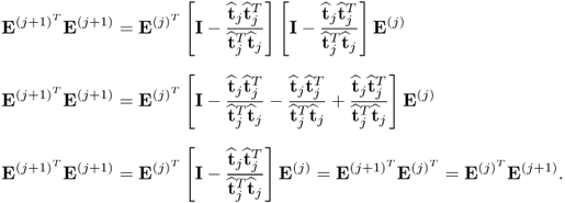
2. The t-score vectors are mutually orthogonal.
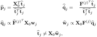
3. The matrix vector products

and

are equivalent.
4. The matrix-vector product

for all
i <
j.
5. The ith t-score and the jth u-score vectors are orthogonal for all i < j.
6. It is sufficient to either deflate the input or the output data matrix.
7. The w-weight vectors are mutually orthonormal.
8. The ith w-weight vector and the jth p-loading vector are orthogonal for all j > i and equal to 1 if i = j.
9. The value of the regression coefficient
bj is equal to the length of the

-loading vector.
10. The
jth q-weight and

-loading vector point in the same direction.
11. The t-score variables are asymptotically Gaussian distributed.
12. The PLS q-weight and p-loading vectors and the value of the objective function λ
j allow reconstructing

.
13. If the covariance matrix

has full rank
nx and the maximum number of latent variable sets have been computed, the PLS regression matrix between the input and output variables,

, is equivalent to that calculated by the ordinary least squares solution,

.
14. In contrast to ordinary least squares, PLS does not require a matrix inversion to compute the regression matrix

.
15. Comparing with the algorithm, discussed in the previous subsection, the computation of a PLS model can be considerably simplified leading to a computationally efficient algorithm.
The above properties are now formulated mathematically and proven.
Property 10.4.1 – Singular value decomposition of  .
.
If the cross-covariance matrix

is available, there exists the following relationship between the
jth pair of weight vectors and the maximum of the objective function for determining these vectors.
Theorem 10.4.1
The weight vectors wj and qj and the value of the objective function in (10.6), λj, are the left and right singular vector and the largest singular value of the singular value decomposition of  , respectively (Kaspar and Ray 1993).
Proof.
Equation (
10.10a) shows that the weight vectors
wj and
qj are the dominant eigenvectors of

and

, respectively. Moreover, the largest eigenvalue of both matrices is

. On the other hand, a singular value decomposition of a matrix

of arbitrary dimension is equal to

, where the column vectors of

, that is, the left singular vectors, are the eigenvectors of

, the column vectors of

, that is, the right singular vectors, are the eigenvectors of

, and the elements of the diagonal matrix

are the square root of the eigenvalues of

or

(Golub and van Loan 1996). Note that the eigenvectors of

or

are scaled to unit length. Now, replacing

with

, it follows that the first column vector of

is
wj, the first column vector of

is
qj and square root of the eigenvalue of

or

is λ
j, is the first diagonal element of

, that is, the largest singular value of

. This largest singular value, however, is equal to the maximum of the objective function in (
10.6), which concludes this proof.
Property 10.4.2 – Orthogonality of the t-score vectors.
The pair of t-score vectors

and

has the following geometric property.
Theorem 10.4.2
The t-score vectors  and
and  , i ≠ j, are mutually orthogonal, that is
  .
.
Proof.
First, revisiting the determination of the kth pair of loading vectors yields
10.19 
With respect to (
10.15a), utilizing (
10.19) gives rise to the following deflation procedure for
E(j) and
F(j)10.20 
The deflation procedure can, alternatively, also be carried out as
10.21 
Next, applying the above expressions for deflating E(j) to simplify the expression
10.22 
by assuming that i < j, yields
10.23 
Now, substituting (
10.23) into (
10.22) gives rise to
10.24 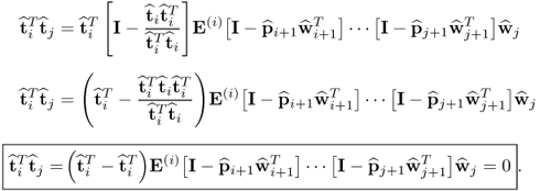
It is interesting to note that the orthogonality property of the t-score vectors implies that the estimated covariance matrix of the score variables is a diagonal matrix
10.25 
The orthogonality property of the t-score vectors also results in interesting geometric properties in conjunction with the deflated matrix E(j), which is discussed next.
Property 10.4.3 – Matrix-vector products  and
and  .
.
The mutual orthogonality of the t-score vectors gives rise to the following relationship for the matrix vector products

and

.
Lemma 10.4.3
The products  and
and  are equivalent
Proof.
Using the deflation procedure to compute E(j) yields
10.26 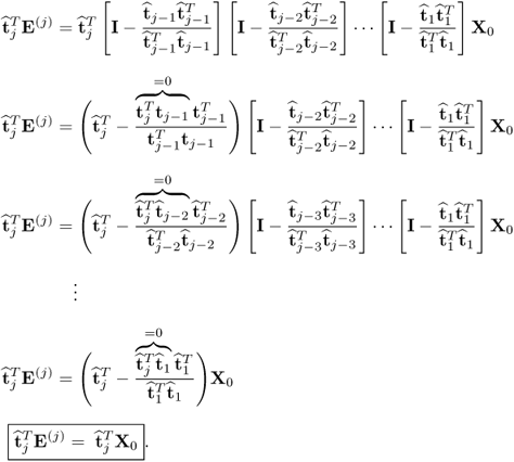
Property 10.4.4 – Matrix-vector product  .
.
The mutual orthogonality of the t-score variable leads to the following property for the matrix-vector product

if
i <
j.
Lemma 10.4.4
The matrix vector product  for all i < j and
  for all i ≥ j.
Proof.
For i < j, the application of the deflation procedure for E(j) gives rise to
10.27 
Substituting the above equation into the matrix-vector product

yields
10.28 
For i ≥ j, Lemma 10.4.3 highlights that

. Equation (
10.19) shows that

forms part of the calculation of the p-loading vector
10.29 
Property 10.4.5 – Orthogonality of the t- and u-score vectors.
The mutual orthogonality of any pair of t-score vectors also implies the following geometric property for the t- and u-score vectors.
Lemma 10.4.5
The ith t-score vector is orthogonal to the jth u-score vector, that is,  for all i < j.
Proof.
With

, the scalar product

becomes
10.30 
For j > i, tracing the deflated output matrix F(j) from j back to i gives rise to
10.31 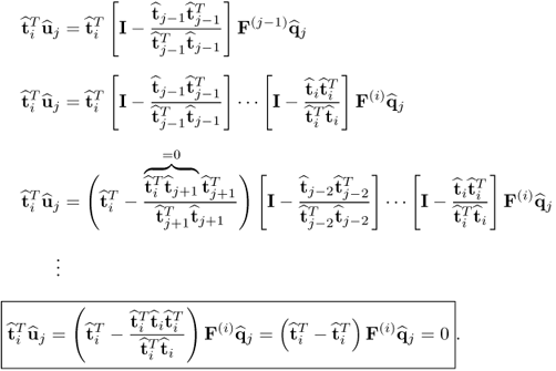
Property 10.4.6 – Deflation of the data matrices.
The analysis focuses now on the deflation procedure, which yields that only one of the output variable sets needs to be deflated and not both simultaneously. Therefore, the following holds true for the deflation of the data matrices.
Theorem 10.4.6
The deflation procedure requires the deflation of the output data matrix or the input data matrix only.
Proof.
First, we examine the deflation of the output data matrix. This analysis also yields the necessary condition to show that it is sufficient to deflate the input data matrix only, which culminates in Corollary 10.4.8. Examining the deflation procedure of the PLS algorithm in
Table 10.1 highlights that the deflation procedure is applied to the covariance and cross-covariance matrices. These matrices can be replaced by the matrix products

and

, respectively. The deflation of these matrix products leads to
10.32 
If
j = 1, it follows from (
10.32) that

. To prove the general case, the deflation procedure allows computing
E(j) from the output data matrix
X0 using the score vectors

, … ,

.
10.33 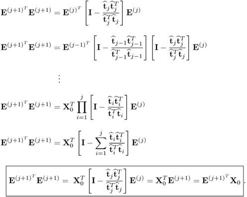
The above relationship relies on the fact that the t-score vectors are mutually orthogonal, as described in Theorem 10.4.2, and that

for all
i <
j, outlined in Lemma 10.4.4. Applying the same steps yields
10.34 
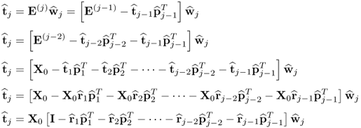
The conclusion of this proof requires showing that the calculation of the t-score vectors can be carried out directly from the input data matrix, since
10.35 
which is formulated below.
Lemma 10.4.7
The definition of the r-weight vectors
10.36 
enables calculation of the t-score vectors directly from the input data matrix, that is,  , 1 ≤ j ≤ n.
Proof.
Revisiting the calculation of the kth t-score vector yields
10.37 
which gives rise to the following iterative calculation of the r-weight vectors
10.38 
Equation (
10.35) highlights that only the output matrix

needs to be deflated, given that the r-weight vectors allow the computation of the t-score vectors directly, which concludes the proof of Theorem 10.4.6. Moreover, it is also important to note the following.
Corollary 10.4.8
It is also sufficient to deflate X0 instead of  .
.
Corollary 10.4.8 follows from the fact that  , discussed in (10.34). Whilst this does not require the introduction of the r-weight vectors in Lemma 10.4.7, it requires the deflation of two matrix products, that is,
  and
and  , for computing the pairs of weight and loading vectors. It is, however, computationally more expensive to deflate both matrix products. The following rank-one modification presents a numerically expedient way to deflate the matrix product
10.39 
It should be noted that the scalar product  is required for the calculation of the loading vectors and hence available for the deflation of
  . The relationship of (10.39) relies on (10.19), (10.29) and (10.32).
Property 10.4.7 – Orthogonality of the w-weight vectors.
We now focus on orthogonality properties of the w-weight vectors and start with the geometry property of any pair,

and

, which has the following property.
Theorem 10.4.9
The w-weight vectors  and
and  , i ≠ j, are mutually orthonormal, that is
  .
.
Proof.
Assuming that
i >
j, the scalar product

can be rewritten as
10.40 
which follows from (
10.10a). Next, analyzing the term

reveals that it is equal to zero
10.41 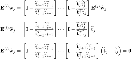
which implies that

Property 10.4.8 – Orthogonality of the w-weight and p-loading vectors.
The following holds true for the scalar product

.
Lemma 10.4.10
The ith p-loading and the jth w-weight vector are orthogonal if i > j and equal to 1 for i = j.
Proof.
According to (
10.19), the scalar product

is given by
10.42 
For i > j, tracing the deflation procedure for E(i) from i back to j yields
10.43 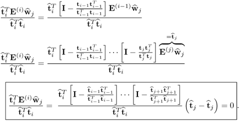
That

for
i =
j follows from the computation of the p-loading vector
10.44 
Property 10.4.9 – Calculation of the regression coefficient  .
.
There is the following relationship between the estimated regression coefficient of the
jth pair of score variables,
tj and
uj, and the length of the
jth

-loading vector
Proof.
Determining the length of

yields
10.45 
However, since

is the dominant eigenvector of

, the expression

is equal to the largest eigenvalue. According to (
10.6) and (
10.10a) this eigenvalue is equal to the square of the Lagrangian multiplier of the objective function for computing the
jth pair of weight vectors. Moreover, the eigenvalue of

is (
K − 1)
2 times the eigenvalue of

,

, and hence, equal to

. On the other hand,

is the estimate for
K − 1 times the covariance between the t- and u-score variables. Consequently, (
10.45) becomes
10.46 
which is, according to (
10.11), equal to the estimate

.
Property 10.4.10 – Relationship between the q-weight and  -loading vectors.
The following relationship between the
jth pair of q-weight and

-loading vectors exists.
Proof.
According to (
10.8), the q-weight vector can be written as
10.47 
whilst the

-loading vector is given by
10.48 
Since
10.49 
is, according to Theorem 10.4.11, equal to

. Equation (
10.48) therefore becomes
10.50 
This, however, implies that

, where the scaling factor between both vectors is the regression coefficient

.
Property 10.4.11 – Asymptotic distribution of t-score variables.
Equations
2.23 and
2.24 describe the data structure for PLS models, which gives rise to the following asymptotic distribution of the t-score variables.
Theorem 10.4.13
Under the assumption that the source variables have zero mean and are statistically independent, the t-score variables asymptotically follow a Gaussian distribution under the Liapounoff theorem, detailed in 9.31, since
10.51 
Proof.
The calculation of the t-score variables
10.52 
becomes asymptotically
10.53 
Replacing
rj,

and
e by
pj,

and
g, respectively, (
10.52) shows the same formulation as that for computing the t-score variables using PCA. Consequently, the proof of Theorem 9.3.4 is also applicable to the proof of Theorem 10.4.13.
Property 10.4.12 – Reconstruction of the Cross-covariance matrix  .
.
The focus now shifts on the reconstruction of the cross-covariance matrix

using the sets of LVs computed by the PLS algorithm.
Theorem 10.4.14
If the covariance matrix  has full rank nx, the nx sets of LVs allow a complete reconstruction of the cross-covariance matrix
  using the nx p-loading vectors, the nx value of the objective functions function and the nx q-weight vectors.
Proof.
The reconstruction of the covariance matrix

follows from
10.54 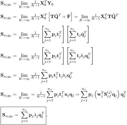
The above holds true, since:
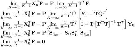
;
- the t-score vectors are mutually orthogonal, which Theorem 10.4.2 outlines;
 , which Theorem 10.4.11 confirms;
 which follows from (10.11); and
 which follows from (10.9).
Property 10.4.13 – Accuracy of PLS regression model.
The following relationship between the PLS regression model and the regression model obtained by the ordinary least squares solution exists.
Theorem 10.4.15
Under the assumption that the rank of the covariance matrix  is nx the PLS regression model is identical to that obtained by an ordinary least squares solution, that is
  .
.
Proof.
Starting by revisiting the data structure in
2.2310.55 
Using PLS, the prediction of output vector y0 becomes
10.56 
Next, analyzing the relationship between

and

as well as between

and

concludes this proof, since
10.57 
which gives rise to
10.58 
With
RR−1 =
R−TRT reducing to the identity matrix, (
10.58) becomes
10.59 
Property 10.4.14 – Computing the estimate of  .
.
Using the
nx sets of LVs, computed from the PLS algorithm, the following holds true for estimating the parameter matrix

,

.
Lemma 10.4.16
If the covariance matrix  has full rank nx, the nx sets of LVs allow one computation of an estimate of the parameter matrix
  without requiring the inversion of any squared matrix.
Proof.
The prediction of the output vector y0 using the nx sets of LVs is
10.60 
The column vectors of the matrices

and
R, however, can be computed iteratively
10.61 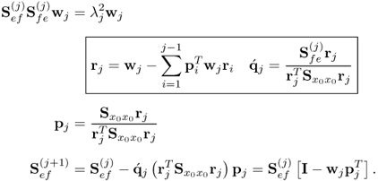
The expression for determining the q-loading vector follows from (
10.35) and (
10.37). Hence, unlike the OLS solution, PLS does not require any matrix inversion to iteratively estimate

. Subsection 6.2.2 presents an excellent example to demonstrate the benefit of the iterative PLS procedure over OLS.
Property 10.4.15 – Computationally efficient PLS algorithm.
The preceding analysis into the properties of PLS algorithm has shown that the deflation procedure only requires the deflation of the input or the output data matrix and that introducing the r-weight vectors allows the t-score vectors to be be directly computed from the input data matrix. This gives rise to the development of a computationally efficient PLS algorithm.
Table 10.2 shows the steps of the revised PLS algorithm. To cover any possible combination in terms of the number of input and output variables
nx and
ny, the revised algorithm includes the case of
ny = 1 and obtains the w-weight or the q-loading vector using the iterative power method, depending on whether
nx <
ny or n
x ≥ n
y, respectively. More precisely, the dimension of the symmetric and positive semi-definite matrix products

and

are n
x × n
x and n
y × n
y, respectively. Given that there is the following linear relationship between the weight vectors
10.62 
only one of the dominant eigenvectors needs to be computed. It is therefore expedient to apply the power method to the smaller matrix product if n
x ≠ n
y. If
ny = 1, the covariance matrix

reduces to a vector of dimension
nx. In this case, the w-weight vector is proportional to

. It should be noted that the algorithm in
Table 10.2 assumes the availability of the covariance and cross-covariance matrices

and

. As they are not available in most practical cases, they need to be estimated from the recorded samples stored in
X0 and
Y0 and the computed weight and loading vectors become, accordingly, estimates. It should also be noted that the PLS algorithm in
Table 10.2 is similar to that reported in Dayal and MacGregor (1997a).
Table 10.2 Computationally efficient PLS algorithm
| 1 |
Initiate iteration |
j = 1,  |
|
|
 |
| 2 |
Set up matrix product |
if nx < ny else |
|
|
 |
| 3 |
Check dimension of y0 |
if ny = 1,  and go and go |
|
|
to Step 9, if not go to Step 4 |
|
|
 |
| 4 |
Initiate power method |
if nx < ny else |
|
|
 |
|
|
1wj = Mw(0wj) |
| 5 |
Compute matrix-vector product |
if nx < ny else |
|
|
1qj = Mq(0qk) |
|
|
 |
| 6 |
Scale weight vector |
if nx < ny else |
|
|
 |
|
|
if ||1wj − 0wj|| > ϵ |
|
|
or ||1qj − 0qj|| > ϵ |
| 7 |
Check for convergence |
0wj = 1wj or 0qj = 1qj and |
|
|
go to Step 5 else set wj = 0wj |
|
|
or qj = 0qj and go to Step 8 |
|
|
 |
| 8 |
Calculate 2nd weight vector |
if nx < ny else |
|
|
 |
| 9 |
Compute r-weight vector |
 |
| 10 |
Determine scalar |
 |
| 11 |
Calculate p-loading vector |
 |
| 12 |
Obtain  -loading vector -loading vector |
 |
| 13 |
Deflate cross-covariance matrix |
 |
| 14 |
Check whether there is significant |
If so, go to Step 15 |
|
variation left in  |
if not go to Step 16 |
| 15 |
Check for dimension |
If j < nx, set j = j + 1 and go to |
|
|
Step 2, if not go to Step 16 |
| 16 |
Compute regression matrix |
 |
10.5 Properties of maximum redundancy PLS
Section 2.3 introduces MRPLS as a required extension to PLS to model the data structure in 2.51. This section offers a detailed examination of MRPLS in term of its geometric properties and develops a numerically more efficient algorithm. Readers who are predominantly interested in the application of the methods discussed in this book can note the computationally efficient MRPLS algorithm in Table 10.3 or the batch algorithm for simultaneously computing the n q-loading and w-weight vectors in Table 10.4.
Table 10.3 Computationally efficient MRPLS algorithm
| 1 |
Initiate iteration |
n = 1, j = 1 |
|
|
 , , |
| 2 |
Set up matrix products |
 and and |
|
|
 |
| 3 |
Set up initial q-weight vector |
 |
| 4 |
Compute auxiliary weight vector |
 |
|
|
if j = n |
| 5 |
Calculate w-weight vector |
 |
|
|
else :  |
| 6 |
Determine q-weight vector |
 |
|
|
if  |
| 7 |
Check for convergence |
set  and go to Step 4 and go to Step 4 |
|
|
else set  and go to Step 8 and go to Step 8 |
|
|
if j = n :  |
| 8 |
Compute r-weight vector |
else : |
|
|
 |
|
|
if j = n :  |
| 9 |
Determine p-loading vector |
else compute  and and |
|
|
 |
|
|
if j = n  |
| 10 |
Determine  -loading vector -loading vector |
else |
|
|
 |
|
|
if j = n  |
| 11 |
Deflate cross-product matrix |
else |
|
|
 |
|
Check whether there is |
if so j = j + 1, n = n + 1 |
| 12 |
still significant variation |
and go to Step 4 |
|
remaining in  |
if not j = j + 1, go to Step 13 |
| 13 |
Check whether j = nx |
if so then terminate else go to Step 3 |
Table 10.4 Simultaneous MRPLS algorithm for LV sets.
| 1 |
Form matrix products |
 and and  |
| 2 |
Compute SVD of  |
 |
| 3 |
Form matrix product |
 |
| 4 |
Form matrix product |
 |
| 5 |
Calculate SVD of S |
 |
| 6 |
Determine w-weight matrix |
 |
| 7 |
Compute q-weight matrix |
 |
| 8 |
Calculate w-loading matrix |
 |
| 9 |
Obtain  -loading matrix -loading matrix |
 |
The analysis of the properties of the MRPLS algorithm concentrates on the geometric properties of score, loading and weight vectors first. The results enable a further analysis regarding the deflation procedure and contribute to the numerically and computationally efficient algorithm that is summarized in Table 10.3.
It should be noted that the proposed MRPLS algorithm in Table 2.3 incorporates the fact that only one of the matrices needs to be deflated and that the length-constraint for the w-weight vectors  is equal to
  . This is also proven in this section as part of the analysis of the deflation procedure.
The properties of the MRPLS algorithm are as follows.
1. The t-score vectors are mutually orthonormal.
2. The t- and u-score vectors are mutually orthogonal.
3. The products

and

are equal to

and

, respectively.
4. The w-weight, the auxiliary w-weight and p-loading vectors are mutually orthogonal.
5. The q-weight vectors are mutually orthonormal and point in the same direction as the

-loading vectors.
6. The constraint of the MRPLS objective function

is equal to

.
7. The MRPLS objective function

is equal to

.
8. The w-weight and auxiliary w-weight vector are the left and right eigenvectors of

.
9. The q-weight vectors are right eigenvectors of the

.
10. The w- and q-weight vectors can be simultaneously and independently computed as the left eigenvectors of the matrix products

and

, respectively.
Property 10.5.1 – Orthogonality of the t-score vectors.
The first property relates to the geometry of the t-score vectors, which Theorem 10.5.1 describes.
Theorem 10.5.1
The t-score vectors are mutually orthonormal, that is,  .
.
Proof.
The proof for Theorem 10.5.1 requires a detailed analysis of the deflation procedure and starts by reformulating

10.63 
Now, incorporating the deflation procedure for the data matrix

yields
10.64 
under the assumption that i < j. Applying the deflation procedure a total of j − i − 1 times yields
10.65 
The vector-matrix product to the left, however, reduces to

, which implies that

if i ≠ j and 1 if
i =
j.
Property 10.5.2 – Orthogonality of the t- and u-score vectors.
The t- and u-score vectors have the following geometric property.
Theorem 10.5.2
The t- and u-score vectors are mutually orthogonal, that is, 
Proof.
The proof of

commences with
10.66 
Assuming that i < j and applying the deflation procedure for E(j) a total of j − i − 1 times gives rise to
10.67 
Equation (
2.70) yields that

, which yields
10.68 
and hence
10.69 
The above conclusion, however, is only valid for
i <
j. For the case of
i >
j, (
10.66) can be rewritten as follows
10.70 
Given that the t-score vectors are mutually orthonormal, the matrix-vector product on the right hand side of (
10.70) reduces to
10.71 
Finally, for
i =
j, (
10.69) yields

. Hence,

.
Property 10.5.3 – Matrix products  and
and 
The analysis of the geometric properties of the t- and u-score variables is now followed by examining the effect that mutually orthonormal t-score variables have upon the deflation procedure. Lemma 10.5.3 describes this in detail.
Lemma 10.5.3
The mutually orthonormal t-score vectors simplify the deflation step to guarantee that only one of the cross product matrices needs to be deflated, that is,  and
and  .
.
Proof.
Starting with the deflation of the input data matrix, which is given by
10.72 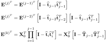
where

. Similarly, the deflation of
F(j) is given by
10.73 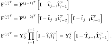
Next, incorporating the above deflation procedures gives rise to
10.74 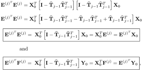
respectively. It follows from Lemma 10.5.3 that
10.75 
According to Theorem 10.5.1,

.
Property 10.5.4 – Orthogonality of the weight and vectors of the input variables.
Starting with the orthogonality properties of the weight and loading vectors associated with the input variables, Theorem 10.5.4 highlights the geometric relationships between the weight and loading vectors.
Proof.
The first step is to show that

, which follows from
10.76 
It is therefore sufficient to prove

, as this includes the case

for all i ≠ j. Given that

,

can be written as
10.77 
Theorem 10.5.1 confirms that (
10.77) is δ
ij.
Property 10.5.5 – Orthogonality of the q-weight and  -loading vectors.
With regards to the weight and loading vectors of output variables, Theorem 10.5.5 summarizes the geometric relationships between and among them.
Theorem 10.5.5
The q-weight vectors are mutually orthonormal and the q-weight and  -loading vectors are mutually orthogonal, i.e.
  for all i ≠ j.
Proof.
Substituting the relationship between the w- and q-weight vectors, that is,

, into

under the assumption that
i <
j, gives rise to
10.78 
Given that  and
and  , for all i ≠ j, (10.78) reduces to
  . Next, that
  for all i ≠ j follows from
10.79 
Hence,
10.80 
and consequently
10.81 
which completes the proof of Theorem 10.5.5.
Property 10.5.6 – Simplification of constraint  .
.
Theorem 10.5.4 can be taken advantage of to simplify the constraint for the w-weight vector

, which is discussed in Lemma 10.5.6.
Lemma 10.5.6
The constraint  is equal to
  .
.
Proof.
Lemma 10.5.3 highlights that

is equal to

. Next, incorporating the fact that the w-weight and the p-loading vectors are mutually orthonormal (Theorem 10.5.4) gives rise to
10.82 
Property 10.5.7 – Simplification of the MRPLS objective function.
Theorem 10.5.4 and Lemmas 10.5.3 and 10.5.6 yield a simplification for solving the MRPLS objective function, which is described in Theorem 10.5.7.
Theorem 10.5.7
The relationships of the MRPLS objective function,

with respect to w and q,

are equal to

respectively.
Proof.
Directly applying Lemmas 10.5.3 and 10.5.6 to the solution of the MRPLS objective function yields
10.83 
Next, incorporating the results described in Theorem 10.5.4 to the matrix-vector product

gives rise to
10.84 
Consequently,

Property 10.5.8 – Relationship between weight vectors for input variables.
Theorem 10.5.8 describes the relationship between the
jth w-weight vector,

, and the
jth auxiliary weight vector

.
Theorem 10.5.8
The jth w-weight and auxiliary weight vectors are the left and right eigenvectors of the matrix product  , respectively.
Proof.
That

is the left eigenvector of

, associated with the largest eigenvalue, can be confirmed by solving the relationships of the MRPLS objective function
10.85 
which yields
10.86 
According to the MRPLS algorithm in Table
2.3, the auxiliary weight vector,

, is initially determined as the matrix-vector product

. By substituting Steps 4 to 8 into Step 3 yields
10.87 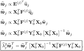
Therefore,

is the dominant right eigenvector and

is the dominant left eigenvector of

.
Property 10.5.9 – Calculation of the kth q-weight vector.
Before introducing a computationally efficient MRPLS algorithm, Lemma 10.5.9 shows that q-weight and

-loading vectors are also eigenvectors of a specific matrix product.
Proof.
Lemma 10.5.9 directly follows from the relationships of the MRPLS objective function in (
10.85)
10.88 
Substituting the equation on the left hand side into that of the right hand side yields
10.89 
Property 10.5.10 – Computationally efficient MRPLS algorithm.
After discussing the geometric orthogonality properties of the weight, score and loading vectors as well as their impact upon the deflation procedure, a computationally efficient MRPLS algorithm can now be introduced.
Table 10.3 summarizes the steps of the implementation of the revised MRPLS algorithm. Computational savings are made by removing the calculation of the score vectors and reducing the deflation procedure to the rank-one modification

. Finally, this section concludes with the development of a batch algorithm for simultaneously computing the
n q- and w-weight vectors.
Simultaneous computation of weight vectors
Recall that the derivation of the MRPLS algorithm in Subsection 2.3.3 consists of two steps. The first step involves the computation of the q-loading vectors by solving 2.63. The second step subsequently determines the w-weight vector by solving 2.66. It has then been shown that both steps can be combined. More precisely, the solution of the combined objective function in 2.68 is equivalent to the individual solutions of 2.63 and 2.66.
Coming back to the facts (i) that the q-weight vectors can be determined independently from the w-weight vectors and (ii) that the jth q-weight vector is the dominant eigenvector of the matrix  gives rise to the following theorem.
Theorem 10.5.10
The kth q-weight vector is the eigenvector associated with the kth largest eigenvalue of  , which is a symmetric and positive semi-definite matrix of rank n ≤ ny.
Proof.
The proof of Theorem 10.5.10 commences by showing that the matrix product

is of rank n ≤ n
y. With regards to the data structure in
2.51, the covariance and cross-covariance matrices

and

are equal to
10.90 
and
10.91 
respectively. The matrix products

and

are equal up to the scaling factor
K − 1. As the rank of the true cross-covariance matrix is
n, given that

,

and

, the rank of

is asymptotically
n, under the assumption that
Sss has full rank rank
n, that is, the source signals are not linearly dependent. The
jth q-weight vector is an eigenvector associated with the eigenvalue

, which suggests a different deflation for

. Abbreviating this matrix expression by

and defining

, the first q-weight vector satisfies
10.92 
Given that

is symmetric and positive definite, the deflation procedure for determining the second q-weight vector that is orthogonal to the first one is as follows
10.93 
which is the principle of the power method to determine subsequent eigenpairs of symmetric and positive definite matrices. After determining the jth eigenpair, the deflation procedure becomes
10.94 
accordingly. Given that the rank of

is
n, a total of
n eigenpairs can be determined by the iterative power method with deflation. On the other hand, the
n eigenvectors and eigenvalues can also be determined simultaneously in a batch mode, for example discussed in Chapter 8 in Golub and van Loan (1996). Once the
n q-weight vectors are available, the w-weight vectors can be computed. Before demonstrating that this can also be done in a batch mode, Lemma 10.5.11 shows how to compute the u-scores directly from the output data matrix.
Lemma 10.5.11
If the q-weight vectors are available, the u-score variables can be directly computed from the output data matrix, that is,  .
.
Proof.
In the preceding discussion, the u-score variables have been computed from the deflated output data, that is,

. However, the fact that the q-weight vectors are mutually orthonormal yields
10.95 
The above relationship incorporates

, which (
10.79) highlights.
Next, incorporating  into the objective function for determining the w-weight vector in 2.66 gives rise to
10.96 
Taking advantage of the fact that  and
and  for all i ≠ j, (10.96) can be expanded upon
10.97 

where  . Equation (10.97) can also be written as
10.98 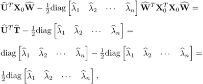
which follows from Theorem 10.5.1 and yields in this batch formulation the same solution as those obtained individually. More precisely, defining the maximum of the combined objective by  , it can only be a maximum if each of the sum elements are a maximum, according to the Bellman principle of optimality (Bellman 1957). As shown in (10.97), storing the n w-weight vectors to form the matrix
  , the solution of the objective function in (10.97) is given by
10.99 
Working out the partial relationships, (10.99) becomes
10.100 
where  and
and  .
.
To simultaneously calculate the n w-weight vectors in batch form, the solution to the objective function in (10.97) is therefore
10.101 
Equations (10.86) and (10.89) outline that the n diagonal elements of the matrix  are equal to the square root of the eigenvalues of
  and
and  . The conclusion of this proof requires to show that
10.102 
To start with, Theorem 10.5.5 shows that  , i.e. the column vectors or
  are mutually orthonormal. Next, (10.83) and (10.84) highlight that
10.103 
which confirms (10.102).
In summary, Theorem 10.5.10 outlined that the q-weight vectors can be simultaneously computed as eigenvectors of the matrix product  , which is positive semi-definite, whose rank asymptotically converges to n ≤ ny. On the other hand, it is also possible to simultaneously compute the w-weight vectors as eigenvectors of the matrix product
  , which is a positive semi-definite matrix with an asymptotic rank of n ≤ ny. Furthermore, the computation of the w-weight vectors is independent of the determination of the q-weight vectors. Equations (10.105) and (10.106) finally summarize the eigendecomposition of these matrices
10.104 
and
10.105 
For canonical correlation analysis (CCA), a multivariate statistical method developed by Harold Hotelling in the 1930s (Hotelling 1935, 1936) that determines weight vectors to produce score variables that have a maximum correlation, a batch algorithm has been proposed to simultaneously determine Q and W. This solution for simultaneously computing the n q- and w-weight vectors can be taken advantage of by simultaneously computing the weight vectors of the MRPLS algorithm. Prior to that, the next paragraph discusses the similarities between the objective functions for CCA and maximum redundancy.
As outlined in Stewart and Love (1968), ten Berge (1985) and van den Wollenberg (1977), the CCA objective function does not consider the predictability of the output variables in the same way as maximum redundancy does. More precisely, the CCA objective function is given by
10.106  Similar to the maximum redundancy formulation, the Lagrangian multipliers are identical and the solution of the CCA objective function for the jth pair of weight vectors, or canonical variates, is given by (Anderson 2003)
10.107 
and
10.108 
It is interesting to note that the difference in the objective function between the CCA and the maximum redundancy is the presence of the matrix product  , which results from the different constraint for the q-weight vector. For the simultaneous computation of the n weight vectors, a batch algorithm that relies on a series of singular value decompositions (SVDs) has been developed (Anderson 2003). Table 10.4 summarizes the steps of the resultant batch algorithm for simultaneously determining the n q- and w-weight vectors.
![]() onto an n-dimensional subspace, n ≤ nx, and show how a sequence of rank-one matrices extract variation from the sets of input and output variables x0 and
onto an n-dimensional subspace, n ≤ nx, and show how a sequence of rank-one matrices extract variation from the sets of input and output variables x0 and ![]() , respectively. Section 10.2 then develops a PLS algorithm and Section 10.3 summarizes the basic steps of this algorithm.
, respectively. Section 10.2 then develops a PLS algorithm and Section 10.3 summarizes the basic steps of this algorithm.![]() and
and ![]() by defining a series of rank-one matrices
by defining a series of rank-one matrices
![]() and
and ![]() with
with ![]() and
and ![]() being mean vectors. In the above equation,
being mean vectors. In the above equation, ![]() and
and ![]() are the rank-one matrices for the input and output matrices, respectively, the n vectors
are the rank-one matrices for the input and output matrices, respectively, the n vectors ![]() are t-score vectors which are estimated from the input matrix,
are t-score vectors which are estimated from the input matrix, ![]() and
and ![]() are estimated loading vectors for the input and output matrices, respectively, and
are estimated loading vectors for the input and output matrices, respectively, and ![]() and
and ![]() are residual matrices of the input and output matrices, respectively. It should be noted that the residual matrices have a negligible or no contribution to the prediction of the output data matrix.
are residual matrices of the input and output matrices, respectively. It should be noted that the residual matrices have a negligible or no contribution to the prediction of the output data matrix.

![]()
![]()
![]()
![]() is the u-score vector of the output matrix, and
is the u-score vector of the output matrix, and ![]() and
and ![]() are the weight vectors for the input and output variable sets, respectively. Finally, according to (10.4a), the score variables, tk and uk, are given by
are the weight vectors for the input and output variable sets, respectively. Finally, according to (10.4a), the score variables, tk and uk, are given by![]() , as well as the set of score variables, tj and uj, make up the jth latent variable set.
, as well as the set of score variables, tj and uj, make up the jth latent variable set.![]() . The optimal solution for the objective function in (10.6) is given by
. The optimal solution for the objective function in (10.6) is given by
![]() . Equation (10.8) also confirms that the two Lagrangian multipliers are identical, since
. Equation (10.8) also confirms that the two Lagrangian multipliers are identical, since![]() . Combining the two expressions in (10.8) gives rise to
. Combining the two expressions in (10.8) gives rise to![]()
![]() and
and ![]() , respectively. The score vectors for E(j) and F(j) can now be computed using (10.4a).
, respectively. The score vectors for E(j) and F(j) can now be computed using (10.4a).![]() -loading vector, which is proven in Section 10.4. For a better understanding of the geometry of the PLS algorithm, however, the introduction of the PLS algorithm here includes this step. Equation (10.11) shows the least squares solution for determining the regression parameter
-loading vector, which is proven in Section 10.4. For a better understanding of the geometry of the PLS algorithm, however, the introduction of the PLS algorithm here includes this step. Equation (10.11) shows the least squares solution for determining the regression parameter![]() . The final step to complete the determination of the jth set of latent variables requires formulation of objective functions for computing the loading vectors
. The final step to complete the determination of the jth set of latent variables requires formulation of objective functions for computing the loading vectors
![]()

![]() -loading vector to be determined as follows
-loading vector to be determined as follows![]() and the cross-covariance matrix
and the cross-covariance matrix ![]()

![]() and
and ![]() (10.15).
(10.15).![]() and the cross-covariance matrix
and the cross-covariance matrix ![]() . The next subsection presents a detailed statistical and geometric analysis of the PLS algorithm and introduces a computationally more efficient algorithm to that described in Table 10.1.
. The next subsection presents a detailed statistical and geometric analysis of the PLS algorithm and introduces a computationally more efficient algorithm to that described in Table 10.1.![]() and the cross-covariance matrix
and the cross-covariance matrix ![]() . This has been for the convenience and simplicity of the presentation. Unless stated otherwise, the analysis that follows, however, removes this assumption and relies on the available data matrices X0 and Y0, whilst acknowledging that the covariance and cross-covariance matrices can be estimated from these data matrices. Hence, the weight, score and loading vectors become estimates.
. This has been for the convenience and simplicity of the presentation. Unless stated otherwise, the analysis that follows, however, removes this assumption and relies on the available data matrices X0 and Y0, whilst acknowledging that the covariance and cross-covariance matrices can be estimated from these data matrices. Hence, the weight, score and loading vectors become estimates.


![]()


![]()


![]() , discussed in (10.34). Whilst this does not require the introduction of the r-weight vectors in Lemma 10.4.7, it requires the deflation of two matrix products, that is,
, discussed in (10.34). Whilst this does not require the introduction of the r-weight vectors in Lemma 10.4.7, it requires the deflation of two matrix products, that is, ![]() and
and ![]() , for computing the pairs of weight and loading vectors. It is, however, computationally more expensive to deflate both matrix products. The following rank-one modification presents a numerically expedient way to deflate the matrix product
, for computing the pairs of weight and loading vectors. It is, however, computationally more expensive to deflate both matrix products. The following rank-one modification presents a numerically expedient way to deflate the matrix product ![]()
![]() is required for the calculation of the loading vectors and hence available for the deflation of
is required for the calculation of the loading vectors and hence available for the deflation of ![]() . The relationship of (10.39) relies on (10.19), (10.29) and (10.32).
. The relationship of (10.39) relies on (10.19), (10.29) and (10.32).![]()

![]()
![]()


![]()


![]()

 ;
; , which Theorem 10.4.11 confirms;
 which follows from (10.11); and
 which follows from (10.9).
![]()
![]()

![]()

![]()
![]() is equal to
is equal to ![]() . This is also proven in this section as part of the analysis of the deflation procedure.
. This is also proven in this section as part of the analysis of the deflation procedure.![]()
![]()


![]()


![]()
![]() and
and ![]() , for all i ≠ j, (10.78) reduces to
, for all i ≠ j, (10.78) reduces to ![]() . Next, that
. Next, that ![]() for all i ≠ j follows from
for all i ≠ j follows from![]()
![]()

![]()
![]()
![]()
![]()

![]()
![]() gives rise to the following theorem.
gives rise to the following theorem.![]()
![]()
![]()
![]()


![]() into the objective function for determining the w-weight vector in 2.66 gives rise to
into the objective function for determining the w-weight vector in 2.66 gives rise to![]() and
and ![]() for all i ≠ j, (10.96) can be expanded upon
for all i ≠ j, (10.96) can be expanded upon
![]() . Equation (10.97) can also be written as
. Equation (10.97) can also be written as
![]() , it can only be a maximum if each of the sum elements are a maximum, according to the Bellman principle of optimality (Bellman 1957). As shown in (10.97), storing the n w-weight vectors to form the matrix
, it can only be a maximum if each of the sum elements are a maximum, according to the Bellman principle of optimality (Bellman 1957). As shown in (10.97), storing the n w-weight vectors to form the matrix ![]() , the solution of the objective function in (10.97) is given by
, the solution of the objective function in (10.97) is given by![]()
![]() and
and ![]() .
.![]()
![]() are equal to the square root of the eigenvalues of
are equal to the square root of the eigenvalues of ![]() and
and ![]() . The conclusion of this proof requires to show that
. The conclusion of this proof requires to show that![]() , i.e. the column vectors or
, i.e. the column vectors or ![]() are mutually orthonormal. Next, (10.83) and (10.84) highlight that
are mutually orthonormal. Next, (10.83) and (10.84) highlight that![]()
![]() , which is positive semi-definite, whose rank asymptotically converges to n ≤ ny. On the other hand, it is also possible to simultaneously compute the w-weight vectors as eigenvectors of the matrix product
, which is positive semi-definite, whose rank asymptotically converges to n ≤ ny. On the other hand, it is also possible to simultaneously compute the w-weight vectors as eigenvectors of the matrix product ![]() , which is a positive semi-definite matrix with an asymptotic rank of n ≤ ny. Furthermore, the computation of the w-weight vectors is independent of the determination of the q-weight vectors. Equations (10.105) and (10.106) finally summarize the eigendecomposition of these matrices
, which is a positive semi-definite matrix with an asymptotic rank of n ≤ ny. Furthermore, the computation of the w-weight vectors is independent of the determination of the q-weight vectors. Equations (10.105) and (10.106) finally summarize the eigendecomposition of these matrices![]()
 Similar to the maximum redundancy formulation, the Lagrangian multipliers are identical and the solution of the CCA objective function for the jth pair of weight vectors, or canonical variates, is given by (Anderson 2003)
![]()
![]()
![]() , which results from the different constraint for the q-weight vector. For the simultaneous computation of the n weight vectors, a batch algorithm that relies on a series of singular value decompositions (SVDs) has been developed (Anderson 2003). Table 10.4 summarizes the steps of the resultant batch algorithm for simultaneously determining the n q- and w-weight vectors.
, which results from the different constraint for the q-weight vector. For the simultaneous computation of the n weight vectors, a batch algorithm that relies on a series of singular value decompositions (SVDs) has been developed (Anderson 2003). Table 10.4 summarizes the steps of the resultant batch algorithm for simultaneously determining the n q- and w-weight vectors.

