Chapter 3
Data Acquisition: Sampling and Data Preparation
Most statistics texts take the facile approach to data, which is to assume that the data were all successfully collected and made ready for analysis before anyone with an interest in statistical analysis came along. The happy result of this view is that the statistics text can usually ignore the thorny issues of where the data come from, how good they are, how they were collected, and how much confidence one can have in them. This text departs from that paradigm, to the extent of talking a little about where data come from, how to get data, and what to do with data before analysis begins. This chapter is devoted to the acquisition of data: sampling and data collection.
3.1 The Nature of Data
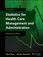
The first thing to be discussed in this chapter is simply the nature of data. Data are the fodder, the raw material of statistical analysis. It is essential to understand two aspects of data in any analysis setting. First, data are recorded in regard to or about cases or observations. Each case or observation represents a record in the data file. Second, data are made up of variables. Each case or observation—each data record—includes one or more measures of the case or record. These are the components of data that are subjected to analysis. For example, Figure 3.1 shows the Excel spreadsheet that was discussed in various ways in Chapter 2. This spreadsheet represents a small data set of 15 observations and 6 variables.
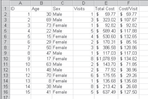
Figure 3.1 A small data set
The observations in Figure 3.1 represent 15 people who may have come to an ambulatory clinic. Each observation appears on a different row of the spreadsheet. The variables in Figure 3.1 are in columns A through F. They include a unique identifier for each observation (ID in column A), the age of the person (Age), the sex of the person (Sex), the number of visits the person has made to the clinic (Visits), a total cost for visits to the clinic for each person (Total Cost), and an average cost per visit (Cost/Visit).
Data are usually displayed and conceived of in the way that is depicted in Figure 3.1. That is, the observations are perceived as occupying rows and the variables are perceived as occupying columns. Observations, it should be pointed out, do not need to be persons. They could be organizations, such as hospitals, health departments, or well-baby clinics. They could be political or geographic entities, such as states, counties, or hospital service areas. But variables always represent some attribute of the observation.
Types of Variables
A general characteristic of variables—at least as far as statistical analysis is concerned—is that they vary. In looking at the data set shown in Figure 3.1, it is easy to see that every variable takes on at least two values (e.g., Sex takes on two), and most take on a different value for each observation. In the unusual event that a variable does not vary—that is, it is a constant—it is useless for statistical analysis. Statistical analysis is almost universally about relating one variable to another. If a variable takes on only one value, it cannot statistically be related to other variables. This idea was discussed in some detail in Chapter 1.
Categorical and Numerical Variables
As also indicated in Chapter 1, variables may be characterized as being two basic types—categorical and numerical. Sex in Figure 3.1 is a categorical variable, classifying each person in the file as male or female. ID is also a categorical variable, classifying each person in the file as a separate entity. Other types of categorical variables could include membership in an HMO; a coding for the seriousness of an emergency, such as yellow and red; the source of coverage for a hospital charge; or blood type.
The remaining variables in the file in Figure 3.1 are numerical data. Again, as introduced in Chapter 1, there are two types of numerical data: discrete and continuous. Discrete numerical data are produced by a counting action and represent measures that can be made in discrete individual units only—never fractions of units. The number of visits to the clinic shown in Figure 3.1 is an example of discrete numerical data. Visits must always be in terms of whole units. Other discrete variables would include the number of persons in an emergency room, the number of unpaid accounts, and the number of immunizations received by a child.
Continuous Numerical Variables
Continuous numerical data are the result of a measurement or a mathematical operation. Age (a measure of the length of time from birth to the present moment) and cost per visit (the result of the division of total cost by the number of visits) are both continuous numerical variables. Other continuous numerical variables include waiting time in an ER or average waiting time, blood pressure, height, temperature, and drug dosage.
The total cost of all visits to the clinic is a little more difficult to classify. When cost is measured in dollars, fractions of dollars (e.g., pennies) might be considered to produce a continuous variable. When measured in pennies, however, each cost is a discrete measure—a result of counting—and cannot be expressed as fractions of pennies. But it is possible, as with height or age, to think of cost as an abstract notion that is approximated (as are height and age) by our measuring tool—in this case, dollars. From this perspective, cost is definitely a continuous variable. But, at the same time, it is possible to say that cost in the abstract is a meaningless concept, and that it becomes meaningful only when measured in some currency; thus, it is a discrete variable. Happily, although we may never resolve this issue, the type of statistics that applies to numerical variables tends to apply equally well to either discrete or continuous variables.
Distinguishing Variables as a Scale
There is a second way, introduced in Chapter 1, of distinguishing variables that refers to the scale upon which they are measured. Scale of measurement is classified as nominal, ordinal, interval, or ratio. The categorical variable Sex in Figure 3.1 is a nominal variable. It names each observation, each person in the file, as male or female. All nominal variables are categorical variables, but not all categorical variables are necessarily nominal variables. They may be ordinal variables or even, possibly, interval variables.
Scale variables can be classified as nominal, ordinal, interval, or ratio.
Ordinal Variables
Ordinal variables are nominal variables, the values of which establish some logical order. For example, young, middle-aged, and old, assigned to three age groups based on the data in Age in Figure 3.1, could be an ordinal variable. An assignment to the young age group might include all three people under 20 (persons with ID 5, 9, and 13). The middle-aged group might include all eight persons from 20 to 50 (persons with ID 1, 4, 6, 7, 8, 11, 15, and 16). Finally, the old group might include the remaining four persons (ID 2, 3, 10, and 12). This variable would be ordered in the sense that there is a logical order assumed by the young, middle-aged, and old. However, there is no assumption that the intervals are equal in any way.
The variable ID in Figure 3.1 is not an ordinal variable. There is no underlying logic to the assignment of 1 to the first person, 2 to the second, and so on. To distinguish one person from another, it would be equally possible to assign C to the first person, 231 to the second, Ralph to the third, and 17 to the fourth. As long as we assign a different code to each, we can keep them separated in our analysis, which is the primary function of an ID. ID, whether it is a number, a letter, or a sequence of nonsense syllables, is a nominal variable.
Interval Variables
Interval variables are ordinal variables that have equal intervals. The categories young, middle-aged, and old are ordinal variables without equal intervals. It would, however, be feasible to create a set of age groupings that contained equal intervals. Suppose we were concerned with a population of Medicare patients and divided their ages into five-year categories, beginning at age 65. If we assign 1 to the first group (ages 65 to 69), 2 to the second group (ages 70 to 74), and so on, we will have created an interval variable.
Ratio variables are interval variables with a true zero point. In the interval measure assigned to the ages of Medicare patients mentioned earlier, there is no true zero point. A 0 would simply mean the age group 60 to 64. It would be possible to create a ratio variable for age in five-year age intervals by beginning with 1 as the ages birth to four. Of course, age measured in one-year intervals is a ratio measure. In Figure 3.1, in addition to Age, the other variables—Visits, Total Cost, and Cost/Visit—are all ratio variables. Each of these variables has equal intervals, and each has a true zero point.
Independent and Dependent Variables
In most statistical analysis, there is a basic assumption that variables are either independent or dependent. Independent variables may often be termed causal variables, whereas dependent variables are considered caused variables. The term “causal variable” is quite commonly employed in statistics and research, but the term “caused variable” is rarely used. Independent variables are typically perceived as variables that are not affected or changed by the other variables under analysis, whereas dependent variables are, as the name implies, assumed to be dependent on or affected by the other variables in the analysis. Independent variables may also be termed predictor variables, because they are perceived to predict the performance of the dependent variables.
Independent variables may be termed causal variables, whereas dependent variables are considered caused variables.
The distinction between independent and dependent variables is not always completely black and white, but with regard to data that are of interest to the health care world, there are some clear types. For example, Figure 3.1 includes two variables—Age and Sex—that are always considered independent variables. It is generally true that age and sex are determined (rather, predetermined) independent of any other variables in a data set. They are also generally perceived as independent of each other.
Conversely, the number of visits to the clinic (Visits) might be determined by age or sex or both. In this context, visits would be a dependent variable. Total cost might also be seen as dependent on age or sex or both, but it is also likely to be dependent on visits. So visits may be dependent relative to age or sex, but they may also be independent relative to total cost. Cost per visit (Cost/Visit) might be seen as dependent on age or sex, but not on visits or total cost. A statistical analysis might show that there is a relationship between either visits or total cost and cost per visit. However, because cost per visit is a composite of visits and total cost (in fact dependent on both because it was created from both), there is no appropriate way to apply statistics to the relationship.
In Chapter 1, we suggested that the “big picture” was that statistics was used to determine whether a value found in a sample could be assumed to have come from a population with certain characteristics. Another way of viewing statistical analysis is to think of it as a means of establishing whether a variable assumed to be dependent on another (assumed independent) can be shown from the data to be so. These two views may seem incompatible, or at least not obviously compatible. However, our discussion of various statistical analyses will attempt to show how the analysis addresses both questions.
Statistics That Apply to Different Types of Variables
As indicated in Chapter 1, this book includes sections on five different basic types of statistical analysis: chi-square statistics, t tests, the analysis of variance (ANOVA), regression, and Logit. The chi-square statistic is designed specifically for data analysis that is limited to categorical data. A chi-square could be used in the case of the data shown in Figure 3.1 to determine, for example, whether there was a relationship, for this data set, between age and sex. However, in order to do this, age would have to be collapsed into two or a few categories. The categories young, middle-aged, and old that were discussed earlier in this chapter could be an example of such an operation. This would result in a new variable that could be used for the chi-square analysis.
The t test can be thought of as a special case of a single dependent variable and a single independent variable. The dependent variable must be numerical and can be measured either on an interval or a ratio scale. The single independent variable can take on only two values and must be categorical. It can be either nominal or ordinal. Thus, a t test could compare, for example, cost per visit for males and females. In this case, cost per visit is the dependent, continuous numerical ratio variable, whereas sex is the single two-value independent variable.
Analysis of variance (ANOVA) can be thought of as a direct extension of the t test to a single categorical, either nominal or ordinal independent variable, that may take on several different values, as opposed to simply two. But analysis of variance may also be extended to include more than one independent variable. In general, however, all independent variables would be categorical and measured either on nominal or ordinal scales. Again, as with the t test, the dependent variable must be numerical—either discrete or continuous—and hence must be measured either on an interval or a ratio scale.
Regression analysis may be thought of as an extension of analysis of variance to numerical independent variables. At the same time, regression analysis does allow the inclusion of categorical variables that take on only two values. The ability to code categorical variables with more than two values as multiple two-value categorical variables extends the utility of regression to encompass almost the entire range of capabilities of analysis of variance. But as with the t test and with analysis of variance, the dependent variable in regression must remain a numerical (discrete or continuous) variable.
Finally, Logit analysis is one of a family of techniques designed specifically to analyze data where the dependent variable is a two-level categorical variable (e.g., the presence or absence of health insurance coverage), whereas the independent variable may be either categorical or numerical.
Much of what has been discussed in the preceding paragraphs will probably not be clear at this time. One of the things this book tries to do is to make these points clear and show how they are important in the use of statistics.
Figure 3.2 represents constructed data (made-up data) for an imaginary clinic. There is an ID for each of the 20 people who are included in the data set, along with nine variables. The variable Age is coded as expected, in years of life. Sex is coded as F or M for female or male. The variable Opinion 1 is the answer to the question (asked on a patient questionnaire) “Do you feel this clinic meets your medical service needs: all the time, most of the time, about as often as not, some of the time, never?” An answer of never was coded 1, some of the time was coded 2, and so on. Opinion 2 is the response to the statement “The service here is better than I would get at a hospital emergency room.” The answers were Strongly agree (coded 5), Agree (coded 4), Undecided (coded 3), Disagree (coded 2), and Strongly disagree (coded 1). The variable Charges represents the charge for the most recent clinic visit for each person. Visit Time represents the amount of time the person was at the clinic, from sign-in to departure. Insurance represents the type of insurance held by the patient, and Prior represents the number of previous times the patient has come to the clinic.
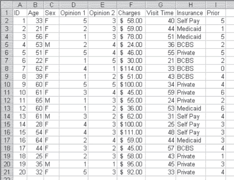
Figure 3.2 Constructed data for an imaginary clinic
3.2 Sampling
All statistical analysis assumes that a sample of some type is under study. Thus the subject of sampling is central to the study of statistics.
Samples and Populations
The term “statistics” is generally used to refer to the subject of this book—that is, the set of calculations that can be used to draw inferences about the relationships between variables and make inferences about populations from samples. “Statistics” is also frequently used as simply the plural of “statistic.” The affinity between these two meanings should be made clear. Statistics is the study of samples, characteristics of samples, and the ways in which inferences about populations may be drawn from those samples. A statistic is a value derived from a sample that can be used to infer something about a population.
Imagine that the data shown in Figure 3.1 represent a 15-person sample. This sample is from some much larger population of all persons who have come to the health center or clinic from which the data had been taken. We can calculate the mean or average of, for example, the number of visits to the clinic. For this sample, the mean comes out to about 3.47 visits per person. This number is a statistic because it came from a sample. We would designate the number ![]() pronounced x-bar, because it was a statistic. The corresponding mean or average for the population from which the sample came would not be called a statistic; it would be a parameter, and it would be designated μ, which is pronounced “mu” and is the lowercase Greek letter μ. This leads to a generally applicable statement: Statistics refer to samples and are designated by lowercase Roman letters; parameters refer to populations and are designated by lowercase Greek letters. As you proceed through this book, you will encounter other measures for both samples and populations that have similar distinctions.
pronounced x-bar, because it was a statistic. The corresponding mean or average for the population from which the sample came would not be called a statistic; it would be a parameter, and it would be designated μ, which is pronounced “mu” and is the lowercase Greek letter μ. This leads to a generally applicable statement: Statistics refer to samples and are designated by lowercase Roman letters; parameters refer to populations and are designated by lowercase Greek letters. As you proceed through this book, you will encounter other measures for both samples and populations that have similar distinctions.
Parameters refer to populations, whereas statistics refer to samples.
The one important contradiction to this general statement about the designation of sample and population values is the designation of size. Sample sizes are universally designated n for number. Population sizes are universally designated N for number. So in the case of the data in Figure 3.1, n is 15, but because we have no information about the size of the population from which the data were drawn, N is unknown.
Drawing a Random Sample from a Population
There are entire books devoted to the subject of sampling, so this treatment will necessarily be only an introduction. But all of the statistics discussed in this text assume at some point that a sample has been taken. Furthermore, as was suggested in Chapter 1, the statistics discussed in this book also assume that the sample selected was either a simple random sample or a systematic sample. This section discusses sampling and sample selection with specific reference to simple random sampling.
It is generally accepted that a person, without some resources other than his or her own intellect, cannot draw a true random sample. No matter how hard we might try, any sample we might draw would be very likely nonrandom. For example, suppose we wish to draw a random sample of 5 persons from a group of 20 people. Suppose further that we also wish to have the sample equally divided into four groups by gender and age at, for example, age 30. This would allow us to have within the overall group a group of five young men, five young women, five older men, and five older women. The basic premise of a simple random sample is that each possible sample that may be selected must have an equal probability of selection as the actual sample.
If we were to try to draw a simple random sample of 5 from this group of 20, we would almost unconsciously end up with a sample that included two men and two women and two older persons and two younger persons. Filling out the five-person sample would be a problem for us because we would be concerned that adding a fifth person would make the sample unrepresentative of the entire group. And herein lies the problem of trying to draw a random sample with no form of external aid. Random samples are not representative; they are random.
Human beings seek to be representative when they try to extract a smaller group from a larger. This inevitably results in the exclusion of many possible combinations of samples that a truly random selection would allow. For example, a person would be very likely not to select five young men as the sample, because the sample would not be perceived as representative of the group of 20 as a whole. But random sampling allows for the selection of the five young men. It is unlikely that it would occur in a random sample, but all statistical analysis is based on the premise that it might happen.
Because the basic assumption of statistics is that a random sample has been selected (and, for the purposes of this book, a simple random sample), it is essential to have some mechanism for making this sample selection. One way to do this would be to assign a number to each member of a population from which a sample is to be drawn. Write each number on a slip of paper. Then put each slip of paper into a large box, shake the box well, and draw out (without looking at the numbers on the paper slips) the number needed. However, this could be both time-consuming and very boring.
Random Number Tables
For years, prior to the common availability of computers, statisticians used a modification of this slip-of-paper technique to draw random samples. They did this by using tables of random numbers, which were published in book form for the specific purpose of drawing random samples. Excerpts from these tables of random numbers are often reproduced in the back of statistics texts, occasionally with instructions on how to use the tables to draw true random samples. Typically, the use of these tables involved the time-consuming task of associating each observation in the population with an entry in the random number table. If that entry was smaller than some predetermined value, the observation in the population would become a member of the sample. For example, if the random number table were divided into three-digit sequences and the population consisted of a thousand observations, to select a 5 percent sample, any observation in the population associated with a three-digit sequence less than 050 would be included in the sample. If the observation were associated with a three-digit sequence larger than 050—for example, 274—that population observation would not be included in the sample.
Random Number Generation via a Spreadsheet: The =RAND() Function
The advent of computers made tables of random numbers obsolete. Even though tables of random numbers continue to be published, it is now many years since anyone has used them to draw random samples. The computer can generate sequences of random numbers and associate them with population observations far faster than we could from a random number table. Excel, as a computer program, is able to generate random numbers in a variety of different ways. This capability allows the Excel user to draw random samples in a variety of different ways, with a great deal of ease and efficiency. Perhaps the simplest of these mechanisms is the =RAND() function.
To employ the =RAND() method of selecting a random sample, it is necessary to have a worksheet reference for each observation in the population. If a researcher desired to draw a random sample from among all the people who work for a state department of health, for example, it would be necessary to have some reference to each of these persons in a spreadsheet. This might be each employee's name on the spreadsheet or, at a very minimum, a number associated with each employee. To continue with the example, suppose names were not on a spreadsheet but were only in an alphabetical hard copy list. Suppose that there are 3,427 employees on the list and we wish to draw a random sample of 100. To draw this sample, we can begin by listing the numbers 1 through 3,427 in column A of a spreadsheet. Do not type each number into 3,427 subsequent cells in column A. Listing the numbers might be done in a couple different ways, but the simplest procedure is probably to put 1 in cell A1 and 2 in cell A2. Then highlight both cells, A1 and A2, and, with the cursor on the lower right corner of the highlighted area (the cursor should appear as a small black cross rather than a large white cross), drag the cursor down to cell A3427. This will probably take 30 seconds or less.
Using the =RAND() Function
Now go back to the top of the spreadsheet and type =RAND() in cell B1. (As was indicated in Chapter 2, it is not necessary to type an Excel function such as =RAND() in caps; lowercase will work just as well.) With =RAND() in cell B1, put the cursor on the lower right corner of the cell (the cursor becomes a small black cross) and double-click. This will fill cells B1 to B3427 with random numbers in the range 0 to 1. Figure 3.3 shows the appearance of the spreadsheet just prior to the double-click that fills column B with random numbers. Column A in Figure 3.3 is the first approximately nine entries in a list that runs to 3,427. When cell B1 is double-clicked with the small black cross on the lower right corner of the cell, the random number represented by the entry in B1 will be copied to the first 3,427 cells in column B.
Figure 3.3 Beginning of random number generation
Now we have a random number associated with each entry in cells A1 through A3427. We could now go down the list of random numbers and include in the sample any entry in column A associated with a random number equal to or less than 0.02918 (100/3427 = 0.02918). But this has two disadvantages.
First, it is still quite time-consuming to review all 3,427 entries. Second, because the generated numbers are random, it is likely that there will be more or fewer than exactly 100 random numbers with values of 0.02918 or less. A more efficient strategy would be to sort the data in column A and column B (the first 3,427 cells in each column) by column B. This will order the data in column A by column B, after which the first 100 cases (or any 100 cases determined a priori) can be selected as the sample. This will not only make the sample selection fast and efficient but also ensure for us a sample of exactly 100 observations.
Working with the =RAND() Function: Random Number Regeneration
One important additional piece of information is needed before you can proceed, however. When the =RAND() function is used to enter values in cells B1 through B3427, what is actually entered into the cells is not a random number but, rather, the random number function. The random number function is regenerated every time the worksheet recalculates. The function also regenerates if an operation, such as sorting, is applied to the worksheet. Consequently, if you sort the data on the column containing the =RAND() function, you will have the unsatisfying result of not seeing the entries in column B appear ordered from lowest to highest, or in any other apparent order, because as soon as the sort occurs, the random number function is regenerated. Hence, the sequence in B will never appear ordered.
Working with the =RAND() Function: Copying the Random Numbers
There is an easy way to get around the problem of recalculation, however, and to feel a little more secure in the result of the sort. After the random numbers have been copied to the first 3,427 cells in column B, while the entire 3,427 cells are still highlighted, select Edit ⇨ Copy, followed by Edit ⇨ Paste Special. In the Paste Special dialog box, click the radio button marked Values. Figure 3.4 shows the Paste Special window with the Values radio button checked. When you click OK and dismiss the dialog box, the formulas in column B, which to this point all show =RAND() in the formula line if you highlight them, will change to the actual numbers shown in the cell. Now both columns A and B can be sorted on column B.
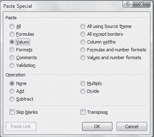
Figure 3.4 Paste Special dialog box
Excel's Sort Routine
The Excel Sort routine is found on the Data Ribbon in the Sort & Filter group. When you invoke the Sort command, you will see the Sort dialog box, shown in Figure 3.5. The Sort command allows for sorting on numerous columns at a time. As shown in Figure 3.5, the sort will be on only one column (column B), and it will be in ascending order. Because there is no label on either column A or column B, the checkbox in front of “My data has headers” is not checked. When you click OK and dismiss the Sort dialog box, the 3,427 numbers in column A will be sorted by column B. The result of this sort is shown in Figure 3.6. Figure 3.6 shows the first 14 rows of the spreadsheet that contain the 3,427 numbers in column A, now sorted on column B. The entry in row 1 of column A is observation 777. This is associated with the smallest random number in column B—0.000152—and is the first observation to be included in the sample of 100. The second observation included is number 1,966, which is associated with the next smallest random number, 0.000288. The last observation in the sample (not shown in the figure) is the observation numbered 3,066, which is associated with the random number 0.030386.
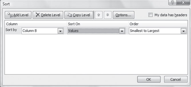
Figure 3.5 Sort dialog box
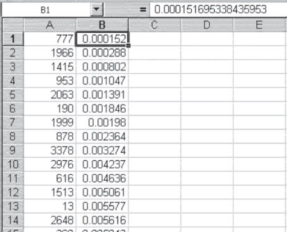
Figure 3.6 Result of sort operation
Now that you've carried out the steps previously discussed, a random set of 100 observations has been selected from among the original 3,427 observations. It remains to the researcher to go to the files and select the employee records corresponding to each of the first 100 numbers in the sample. But the task of selecting the random sample has been completed. This random sample of employees can now be used to calculate any estimates of the total population of employees that one would normally calculate from a random sample.
A Random Sample of Home Health Agency Records
Chapter 1 introduced the problem of the home health agency that wished to do an audit of 10 percent of its 800 records each quarter. The agency had been selecting the records for audit by taking the first record and every tenth record thereafter. It was suggested that perhaps a better way would be to select a simple random sample of records for review. A simple random sample can be selected easily by following the process described previously, in the second subsection of Section 3.2. The records can be put into a consecutive list. Each record can then be given a number from 1 to 800, with this number listed in column A of the spreadsheet. Once the numbers have been listed, each can be assigned a randomly generated number between 0 and 1 using =RAND(). The list can then be sorted on the random number, and the first 80 records can be selected for audit.
Selecting a Sample of Women to Receive a Cancer Education Intervention
Chapter 1 also introduced an example of the use of statistics in which a resident was expected to develop a study in which a sample of women received one type of breast cancer education—a pamphlet. Another sample of women experienced a short talk on breast cancer from a physician and received the pamphlet as well. The question was whether the women who had experienced the talk would show greater knowledge of breast cancer on a brief questionnaire administered after the fact.
For such a study to be effective, it is essential that the women who receive the two different interventions be randomly assigned to the two groups. Suppose the resident hopes to have 30 women in each of the two groups at the completion of the study. However, she does not know who these 60 women are because they are women who will be coming to the clinic in the future.
The easiest way to assign the 60 women randomly to either of the two interventions would be to begin by listing the numbers 1 through 60 in column A of a spreadsheet. Then each of the 60 numbers is assigned a random number using =RAND() in column B. After the Edit ⇨ Copy and Edit ⇨ Paste Special ⇨. Values option is used, the 60 numbers can be sorted by the random numbers. Now the first 30 numbers in the list (those in cells A1 to A30) represent the women who will receive one intervention (e.g., the pamphlet only). In turn, the second 30 numbers (those in cells A31 to A60) represent the women who receive the other intervention (both the pamphlet and the talk).
After the numbers 1 through 60 have been randomly assigned to two groups, the list of those assigned to each group can now be sorted so that they are easier to track. The results of such a sort might be as those shown in Figure 3.7. The figure shows the first 15 women in each of the two groups—those receiving the pamphlet only and those receiving the pamphlet plus the talk. As the figure shows, at the initiation of the study, the first two women seen in the clinic will receive both the pamphlet and the talk. The third woman will receive only the pamphlet, the fourth and fifth women will receive both interventions, and so on. This assignment can be used for the next 60 women coming to the clinic who meet the other study criteria.
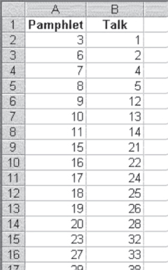
Figure 3.7 Partial list of women who will receive each intervention
There is an important point to be made from Figure 3.7 beyond that of a way of displaying the women who will be selected for each group. It might be noted that the sixth through the eleventh woman arriving at the clinic will be given only the pamphlet. Readers might be tempted to ask how this can be a random ordering if six people in a row are assigned to the same group. This is precisely why humans cannot carry out random selections. We are put off by a sequence of six in a row. But random numbers don't care. And in this case, the sequence of six from 6 to 11 was the result of random selection.
Other Random Sampling Mechanisms: =RANDBETWEEN() and the Data Analysis Add-In
Excel provides a number of different ways to draw random samples. The simplest is the =RAND() method, discussed earlier. A similar way is to use the =RANDBETWEEN (first, second) function, which returns a random integer between the two numbers specified as first and second. If the =RANDBETWEEN() function is to be used, it should be realized that the random numbers selected may be repeated if the range between the two numbers selected as first and second is small. This function recalculates just as =RAND() does, so it is necessary to use the Edit ⇨ Copy and Edit ⇨ Paste Special ⇨ Values sequence prior to sorting if the satisfaction of seeing a sorted list is important.
The Data Analysis Add-In: Random Numbers from Different Distributions
Several other methods of selecting random samples can be found in Excel's Data Analysis add-in. For Excel 2013, look in the Analysis group on the Data Ribbon and choose the Data Analysis option and then the Random Number Generation option in the Data Analysis dialog box. If the Random Number Generation option is invoked in Excel 2013, the Random Number Generation dialog box (shown in Figure 3.8) appears. The Number of Variables field indicates the number of sets of random numbers that are to be generated. In the case shown in Figure 3.8, there will be five sets. The Number of Random Number field indicates the number of random numbers each set will contain. In this case, there will be 10 numbers in each set. The Distribution drop-down list indicates the type of distribution that will be generated. Seven different distributions of random numbers can be generated using this add-in. They are Uniform, Normal, Bernoulli, Binomial, Poisson, Patterned, and Discrete. More will be said of these later.
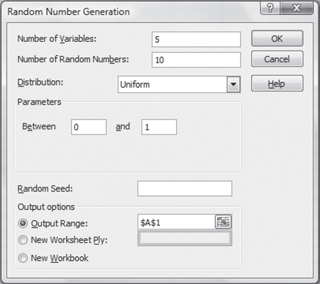
Figure 3.8 Random Number Generation dialog box
For each different type of distribution, corresponding parameters must be specified. For the Uniform distribution, selected in Figure 3.8, the parameters are the two numbers between which the random number will be generated. In the case shown, the numbers will be between 0 and 1, just as generated by the =RAND() function. Any real numbers can be used as the numbers between which random numbers will be generated, but the numbers generated will not be integer values, even if integers such as 5 and 25 are the numbers chosen for the range. Every distribution that can be generated has a separate set of parameters, which will be pointed out as each distribution type is discussed.
Random Numbers Generation: The Random Seed
Each Random Number Generation dialog box allows for the inclusion of a random seed. To understand the random seed, it is necessary to realize that no computer-driven random generating scheme can actually produce true random numbers. Computers can produce what are generally termed pseudorandom numbers. Any pseudorandom number–generating scheme takes some part of the last random number generated and uses that as a seed to begin the generation of the next random number. But in order for this to work, the computer has to have some number to work with as the first seed. Typically, the seed is taken from some source that is constantly changing in no predictable way. In the case of the =RAND() function, the seed is taken from the last several digits of the computer's time clock. These change so rapidly that it is impossible to predict what value they will have when the =RAND() function is invoked.
But the random number–generating schemes in the add-in all begin with a fixed seed by default. This means that every time Excel is started anew, these random number-generating schemes will produce exactly the same string of numbers. This is true for every one of the seven different random number–generating schemes—Uniform, Normal, Bernoulli, Binomial, Poisson, Patterned, and Discrete.
If the random number–generating schemes produced the same set of random numbers every time Excel was started anew, they would not seem to be producing very random numbers. But this problem has a relatively simple solution. Each of the seven random number–generating schemes allows for the specification of a random seed. Before using any of these random number generators, it would be best to use the =RAND() function to generate at least one random number. The first four digits of the result of =RAND() can then be used as an integer (i.e., without the decimal point) and as a random seed in whatever random number generation add-in is being used. Only the first four digits should be used, because the random seed value cannot exceed 9999. This strategy will produce a distinct and different set of random numbers each time the random number–generating schemes are invoked.
Random Numbers from the Uniform Distribution
The Random Number Generation dialog box (see Figure 3.8) will produce a set of random numbers, as shown in Figure 3.9. The 5 in the Number of Variables box has produced 5 columns of numbers, and the 10 in the Number of Random Numbers box has produced 10 rows of numbers. It can be seen that all these numbers are between 0 and 1. It should be further noted that the Uniform distribution generates what are essentially random numbers. In other words, the numbers are generated to nine decimal places. The Uniform distribution was discussed earlier.
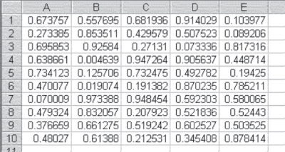
Figure 3.9 Five sets of 10 random numbers
Random Numbers from the Normal Distribution
The Normal distribution dialog box looks exactly like that shown in Figure 3.8, except that in the Parameters field the user is asked to supply the mean and the standard deviation of the distribution. These terms will be discussed in detail in Chapter 6. For the present, it is sufficient to note that the Normal distribution option generates numbers that have no limit. The values generated most likely will be close to the mean value and will vary from the mean value as a function of the value of the standard deviation. The Normal distribution also generates continuous random numbers up to nine decimal places.
Within a spreadsheet, continuous random numbers are generated to nine decimal places.
Random Numbers from the Bernoulli Distribution
The Bernoulli distribution dialog box also resembles Figure 3.8, except for the Parameters field. For the Bernoulli distribution, only one parameter, p, is requested. The p stands for probability and must be between 0 and 1. The Bernoulli distribution option will generate a random sequence of ones and zeros, with the average number of ones being equal to p. So, if you were to generate 10 random ones and zeros using the Bernoulli option with a p of 0.5, it would be like flipping a coin 10 times. You would expect to get five heads (ones) and five tails (zeros), but you would not be surprised if you got four ones and six zeros, or three zeros and seven ones. Because the Bernoulli option generates only 0 or 1, it can be considered as generating discrete random numbers.
Discrete random numbers can take on only integer values (e.g., 0 or 1).
Random Numbers from the Binomial Distribution
The Binomial distribution dialog box requests two parameters—the p value and the number of trials. Again, as with the Bernoulli distribution, the p value refers to the probability of an occurrence. “Number of trials” refers to the number of times the probability will be applied. In the coin-flipping example of the Bernoulli distribution mentioned previously, the number of trials was 10. Rather than generate a series of ones and zeros, the binomial distribution generates a single number between 0 and the number of trials (e.g., 10). That number represents the number of ones that would result from applying p for the number of trial times. In the case of flipping a coin 10 times, the binomial distribution result would be a number between 0 and 10. Because the probability of one's getting a head or a tail is equal, the random numbers generated by the binomial distribution will be predominantly fours, fives, and sixes. The binomial distribution option generates only integer values, so it generates discrete random numbers.
Random Numbers from the Poisson Distribution
The Poisson distribution dialog box requests a single parameter: lambda. “Lambda” refers to the mean value of the distribution, or the average number that will be generated by the distribution over a large number of trials. In a Poisson distribution, the value of lambda is also the variance of the distribution. The Poisson distribution will be discussed further in Chapter 5. The Poisson distribution also generates only integer values, so it, too, generates discrete random numbers.
The patterned distribution is not actually a random number generator at all; rather, it generates a list of numbers that repeat as many times as desired in a pattern that is set by the Parameters field. In terms of the materials in this book, the patterned distribution is not relevant.
Random Numbers from the Discrete Distribution
The discrete distribution requests two parameters: the value and the probability input range. The discrete distribution generates random numbers from a prespecified set of numbers (the value range), according to the probabilities assigned to these numbers (the probability range). So, for example, if the value range was that shown in cells A1 to A10 of Figure 3.10, and the probability range was that shown in cells B1 to B10, the discrete random number generator would generate values of 1 to 10 according to the probabilities shown in column B. It should also be pointed out that the probability range must sum to 1. So if you wanted to generate a random series of, for example, 20 numbers from the list in cells A1 to A10, you would expect, on average, that the random number generation would result in six ones, four twos, two each of three and four, and one each of five through 10. Of course, because this is a random number generation process, it is likely that the result will not be exactly as indicated in the previous sentence. But, in general, the result will be similar to this.
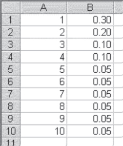
Figure 3.10 Value and probability input range (example)
One point must be made about the random seed in the discrete distribution generator. For some reason, the space following the random seed will be grayed out so that it cannot be used in many instances. The solution is to change to another type of distribution, put in the desired random seed, and then go back to the discrete distribution. The random number generator will pick up the random seed as specified.
It is useful to know of these random number generation capabilities of Excel, in general. However, the material in this book will rely either on the =RAND() method of selecting random samples or, in some examples with regard to the consequences of selection of random samples, on the discrete sampling capability of the random number add-in. In order to provide some familiarity with sampling in general, and these options in particular, the following exercises are offered.
3.3 Data Access and Preparation
Data access can be the subject, just as sampling can, of an entire book. This section provides only a basic introduction to the issues involved. Essentially, data can be accessed and acquired in only two ways; they can be collected directly by the investigator (e.g., the user of this statistics text) or they can be obtained as secondary data. If they are to be collected by the investigator, the options available for collection include questionnaires that are filled out by respondents themselves (e.g., patients or hospital CEOs) or interview schedules to which answers are given by respondents. Direct data collection can also include observation in which the researcher observes and records these specific details on a predetermined schedule.
Secondary Data
Secondary data are data that have been collected for some purpose other than the study of interest to the researcher but can be accessed by the investigator for study purposes. Secondary data could include such information as patients' records (when appropriate clearances for use and informed consent have been obtained), operating data from a hospital or other health care organization, or data in the public domain, such as county-by-county statistics on median income, percentage below poverty, or low birth weight rates.
A major advantage of the use of directly collected data is that data can be collected in a way that is specific to the needs of the investigator. To take a relatively simple example, if the interest is in a patient's age, the investigator can ask the patient for his age. However, if secondary data are used to get a patient's age, the data actually available may not be age but, rather, date of birth. This leads to the general issue of turning those data into data that can be used in the application of other statistical analysis. Happily, Excel is a very useful tool in this process.
An Examination of Data Preparation Using Secondary Data
This section describes an example of the use of Excel in the preparation of some secondary data for analysis. The secondary data to be examined are actual data, but they are data from which all identifying information has been deleted. The data file represents information for 100 hospital discharges for Medicare-eligible persons randomly selected from a much larger file of discharges. There are nine different pieces of information included in the file. These are sex, date of birth, date of hospital admission, date of discharge, MS-DRG code, total hospital charges, actual Medicare payment, number of diagnoses for the hospital stay, and admitting ICD-9 code. (The ICD-9 code is one digit. Normally, ICD-9 codes are three digits or more, but this is the way the data were actually coded and made available, because the institution from which the data came was having trouble coding the ICD-9. Problems such as this are not uncommon in the use of secondary data.)
Importing Data with the Text Import Wizard
The data file is initially in a simple text format, and it must be put into spreadsheet format to be used by Excel. It is not uncommon to find data in a format other than the Excel format. Excel provides a Text Import Wizard with three steps to import text data into Excel. The Text Import Wizard will automatically come up in the Excel screen whenever Excel recognizes that the user is trying to open a text file. The first step of the Text Import Wizard is shown in Figure 3.11.
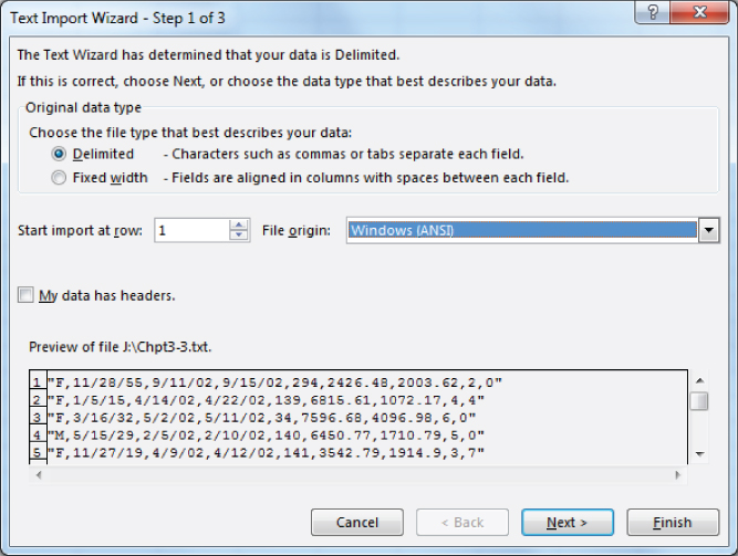
Figure 3.11 Text Import Wizard, Step 1
The Text Import Wizard will assume that the text file to be imported is a data file, as opposed to a conventional text file. It will also assume that each line of the text file represents a separate observation and that individual data elements (the variables) for any observation are all contained on the same line. It will first attempt to determine the way in which each data element is distinguished from every other data element. There are two ways in which data elements may be separated: by using a delimiter or by using a fixed-width field. A delimiter is a character (e.g., a tab or an ampersand) that generally will not be used to represent data but will simply be included in the text file to separate one variable from another. Data may also be stored in a text file in fixed width. Fixed width means that every variable will take up exactly the same number of spaces—for example, 10—in the text file. Delimited data is the most common format. A fixed-width file requires a certain number of spaces for each variable, even though there may be no data in a particular field, or the actual data may be much shorter than the number of spaces allocated. The delimited data file takes up only as much space as is required for each data element.
Step 1
As you can see by the selected radio button in Figure 3.11, the Text Import Wizard has correctly determined, in the case of the data in the text file referenced here, that the data are delimited. The wizard further indicates that the importing of data to the spreadsheet will begin in row 1 and that the text file is actually contained in a Windows (ANSI) format. The other formats that can appear in the file origin window are Macintosh and MS-DOS. The preview area of the dialog box shows the data that will be imported by Excel with the delimiter (in this case, actually a tab character). Line 2 of the preview screen shows F as the first code (representing Female for sex); 1/5/15 representing the date of birth; 4/14/02 and 4/22/02 representing the date of admission and date of discharge, respectively; and 139 representing the MS-DRG code. The remaining information on the first line includes 6815.6 representing the total dollar charges for the stay, 1072.17 representing what Medicare actually paid, 4 indicating four separate diagnoses for the stay, and 4 indicating an admitting ICD-9 code.
Steps 2 and 3
Figure 3.12 shows the second step of the Text Import Wizard. This step allows the user to select the character that is actually used to delimit the data and see the result of the selection of this delimiter in the Data preview area. The check mark before Comma indicates that Excel has correctly determined on its own that the text file was delimited with commas.
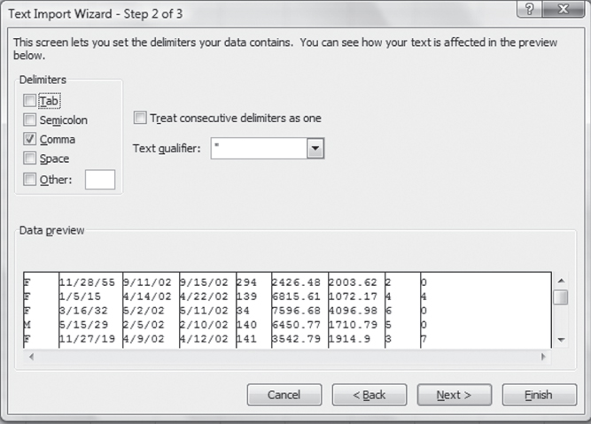
Figure 3.12 Text Import Wizard, Step 2
The final step in the Text Import Wizard is shown in Figure 3.13. This dialog box provides an opportunity to do several things. These include setting the format of each imported column and indicating whether a column should not be imported. The highlighted first column will be acted upon by anything checked in the Column data format area. Each successive column in the data can be highlighted in turn, and its format can be set to General, Text, or Date. General is the most versatile format, as it treats numeric values as numbers, treats text values as text, and treats data in date format (i.e., 11/28/55) as dates.
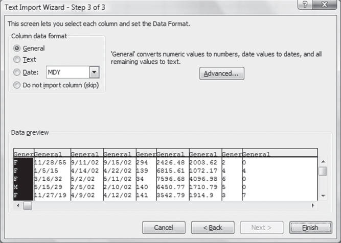
Figure 3.13 Text Import Wizard, Step 3
In general, if Excel correctly recognizes that the data file is delimited (or is of fixed width) and there is no desire to change or delete the actual data elements, it is usually not necessary to go beyond the Step 1 dialog box. In fact, the first dialog box is all that is necessary to convert the file under discussion here to spreadsheet format. If you click the Finish button in the Step 1 dialog box of the Text Import Wizard, the text file will automatically appear as an Excel spreadsheet.
Inspecting, Formatting, and Modifying Imported Data
The data as imported into Excel are shown, in their initial form, in Figure 3.14. Only the first 10 records in the file are shown, although the data file actually contains 100 records. On looking at the file as shown in Figure 3.14, you will immediately notice several things. First, columns B, C, and D contain several cells with number signs (#######) instead of recognizable data. This means that the formatting currently applied to the cell, including its width, is preventing Excel from displaying the data properly. You can correct this situation easily by widening the column (put the cursor between the letters heading any two columns and drag it to the right or double-click). You will also notice as you look at column B that several of the dates (e.g., 5/15/2029, in row 4) have not even occurred yet. But this is the date-of-birth column. Excel has misinterpreted the date 5/15/29 (which obviously meant May 15, 1929) and has made it a complete century later. This problem is one that should be anticipated when using date data that are for a date prior to 1930. Any date prior to that time that is not given as the entire date (i.e., is given only as the last two digits of the year) is treated by Excel on being imported as a date in 20xx rather than a date in 19xx. But because we know that this is a date of birth, it is obvious that we will have to change any dates shown in the imported file as 20xx to dates in the form 19xx.
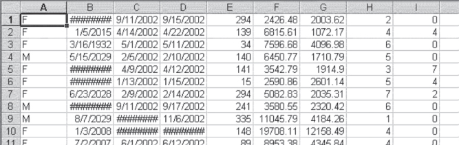
Figure 3.14 Data as initially imported from a text file
Adjusting Dates in Excel
The solution to this problem is a little tricky, but it depends on the fact that Excel stores dates as a number beginning with 1/1/1900 as 1. The number that corresponds to 1/1/2000 is 36526. In order to convert the dates in column B in Figure 3.14 that are given as 20xx to numbers in the form 19xx, it will be necessary to subtract 36525 from each of the dates that are in the form 20xx. Figure 3.15 shows the data from Figure 3.14. The columns containing dates have been widened to show all the dates (no #######). In addition, a column has been inserted between B and C (with column C in Figure 3.14 becoming column D in Figure 3.15) in which the corrected date of birth has been calculated. (In order to insert a column or a row between two other columns or rows, left-click the letter [column] or number [row] where you wish to make the insert. Then right-click the cursor while it is still on the letter or number and select Insert from the pop-up menu. A column will be moved to the left and a new one inserted, or a row will be moved down and a new one inserted.)
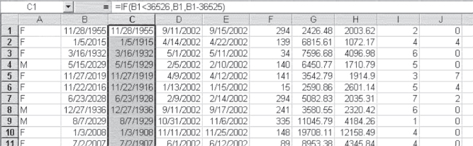
Figure 3.15 Making imported dates century-correct
The =IF() statement that was used to produce the correct date is shown in the formula line of Figure 3.15, and is =IF(B1<36526,B1,B1–36525). The =IF() statement says that if the date given in column B is less than (<) 36526 (i.e., if it is a date prior to 1/1/2000), it should remain as in column B. But if it is not, it should be changed to whatever is in column B minus 36525 (a century of days). There is one small drawback to this strategy. In the unlikely event that a person was actually born in the 1800s rather than in the 1900s, this would change his or her date of birth to a date near the end of the 1900s. This can possibly be checked for in these data, however, because anyone who had a birthdate in the late 1900s would not likely be eligible for Medicare yet. With other types of data, it might be more difficult to determine if a date of birth should be prior to 1900.
Values versus Formulas, Deleting Extra Columns, $ Formatting
Having corrected the date of birth in column C, we should now make several additional modifications to the imported data set. First, the current column C, which gives the corrected date of birth, should be changed from a formula dependent on column B to the value shown in column C. This can be done by right-clicking column C and selecting Copy, then right-clicking column C again and selecting Paste Special ⇨Values for the data in column C (and it can be done while the data are still highlighted, as shown in Figure 3.15). Once this has been done, it is a good idea to eliminate column B by left-clicking the B at the top of the column and then right-clicking and selecting Delete from the pop-up menu. This will put the corrected date of birth in column B. A new first row (row 1) should be added as a place to put an identifier for each variable. A new first column (column A) should be added as a place to put a unique identifier for each hospital stay (an ID number).
Finally, the formatting for the hospital charges and actual Medicare payments can be changed from general to dollar format to clearly appear as dollar amounts. To do this, first highlight the cells that should be in dollar format, in the Home ribbon select the $ pull-down menu from the Number menu, and select the appropriate currency, in this case “$ English (United States)” from the menu. The completed transformation of the data is shown (again, for the first 10 observations only) in Figure 3.16. At this point the data should be saved as an Excel file.
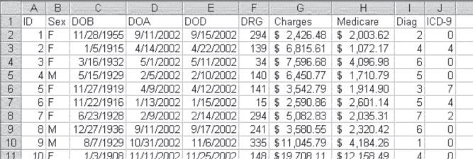
Figure 3.16 Text file imported to Excel with ID and Variable labels
Finally, the formatting for the hospital charges and actual Medicare payments can be changed from general to dollar format to clearly appear as dollar amounts. To do this, first highlight the cells that should be in dollar format and then select Format ⇨ Cells ⇨ Currency. The completed transformation of the data is shown (again, for the first 10 observations only) in Figure 3.16. At this point the data should be saved as an Excel file.
The ID number given in Figure 3.16 (column A) may not seem important, because each record is in a different row and it is not likely that one row will be confused with another. But the ID number can be used to return the data set to the original order if it is sorted on some variable, such as hospital charges or Medicare payments. It can be used to ensure that data stay with the right observation if a subset of observations and variables is moved to another spreadsheet. In general, it is good practice to include an ID number. It takes up little space in a file, and if you do not include it, you will wish that you had.
Performing Data Checks
Usually, importing any data set to Excel and getting it into a format that looks like an Excel spreadsheet (and ensuring that such things as date of birth reflect reality) are not the last step in getting data ready for analysis. In certain cases (e.g., with date of birth), it might be desirable to perform some data checks to see if the data are all within a reasonable range (e.g., not a date that represents one in the future or a date signifying someone was born 100 years from now). We mentioned earlier that in the unlikely event that someone represented in the data file was born before 1900, the method used here to give the correct date of birth would give a date incorrectly recorded as 19xx rather than as 18xx. But this would show up in the data file as a date in the 1990s (assuming that no one is over 112 years of age). So one way to ensure that no one has been incorrectly shown as having been born in the 1990s, when he or she was actually born in the 1890s, is to check the date-of-birth column (DOB) for a date in the 1990s.
Checking Date of Birth with an =IF() Statement
A date in the 1990s in the date-of-birth column can be found simply by looking at each individual entry in column C. But even with only 100 records, this is unnecessarily time-consuming. A better choice is to use the =IF() statement as shown in Equation 3.1.
where C2 references the first data cell in column C (date of birth) and 32874 is the number corresponding to the date 1/1/1990.
This =IF() statement will record a 1 for dates of birth prior to 1990 and a zero for any dates of birth shown as after 1990. The =IF() statement should be put into an unused column in the spreadsheet (e.g., column K). It should then be copied to the end of the data file (in this case, the first 101 rows in the spreadsheet). An easy way to determine if any of the dates are in the 1990s is to sum the column containing the =IF() statement. If the sum is 100, then it is likely that no dates of birth should have been recorded as in the 1800s. If the sum is less than 100, it is easy to find the records for which date of birth should probably have been recorded as 18xx by sorting the entire data set on the column containing the =IF() statement.
In the case of the hospital data being discussed here, none of the dates of birth are recorded as being in the 1990s, so it is probably unlikely that there are any records in the data file with a true date of birth prior to 1900. Once the =IF() statement has done its job of determining if the data in the date-of-birth column are correct, the column containing the =IF() statement can be deleted.
Checking M or F with an =IF() Statement and an =OR() Statement
Other logical checks might be made on the initially imported data. For example, it might be useful to be certain that every entry in the column representing sex is coded either M or F. This can be done by using either the =IF() statement (in this case, a nested =IF() statement) or an =OR() statement. The two statements that can check for either an M or an F in column B are as those shown in Equation 3.2.
or
where B2 references the first data cell in column B.
In the case of the =IF() statement in Equation 3.2, Excel first checks to see if the entry in B2 (or whatever cell is being referenced) is an “F”. The quotation marks are necessary if Excel is to recognize a text character. If Excel finds an “F”, it will put a 1 in the cell in which the =IF() statement appears. If the entry in the referenced cell is not an “F”, Excel then checks to see if it is an “M”. If it finds an “M”, it will record a 1. If Excel finds neither an “F” nor an “M”, it will record a 0. The entries in the column in which =IF() is invoked can then be summed to determine if the sum is equal to the number of observations. If not, the entire data file can be sorted on the =IF() column to find the anomalous data entries in column B. It should be pointed out that “F” and “f” are the same character to Excel, as they are in general to you and to us. So the statement in Equation 3.2 will also find an “f”.
The =OR() statement operates much the same way as =IF(). But it checks both “F” and “M” and if it finds either, it records a TRUE in the column in which it is invoked. If it finds neither “F” nor “M”, it records FALSE. If there are any entries that are not “F” or “M” in the column, recording sex can be determined by counting the number of TRUE entries in the column in which the =OR() statement was invoked. If this is equal to the number of observations, then sex is recorded as “F” or “M” (or “f” or “m”) for each observation. Counting the number of TRUE entries is easier than looking at each entry in the column in which =OR() is invoked. It can be done with the =COUNTIF() function, as shown in Equation 3.3.
where K2:K101 references the data cells in which the =OR() function has been invoked.
Again, once the data checks indicated here have been made, the column in which the check has been carried out can be deleted. This helps keep the data set from becoming cluttered with unneeded information.
Other Possible Data Checks for Medical Data
A number of other data checks might be warranted. These would depend entirely on whether it is possible to specify what codes should appear in given cells. For example, it could be possible to see if date of discharge (in column E) is always later than date of admission (column D). It might be possible to determine if the code given for MS-DRG was, in fact, a legitimate MS-DRG code. But that could require a large number of nested =IF() statements, and it still might not work. Incidentally, it is possible to nest up to 16 =IF() statements.
After you've checked for data errors, it is time to think about the kind of analysis that will be done with the data. As an initial step, it is likely that at some point in any analysis involving this data set, length of hospital stay will be important information. Similarly, it is quite possible that the age of the patient at the time of hospitalization will be of interest. So, at a minimum, these two pieces of information should be developed from what is already in the data.
Calculating Length of Stay (LOS)
Length of hospital stay (LOS) can be determined simply by subtracting the date of discharge (DOD) from the date of admission (DOA). Just as Excel can deal with addition or subtraction in regard to a date and a number, it can also deal with addition and subtraction in regard to two dates. Figure 3.17 shows the calculation of the length of stay in days by subtracting the date in column D from the date in column E (see =E2-D2 in the equation line in the figure). A new column was first inserted between DOD and DRG, and then the subtraction was carried out in the new column F, labeled LOS. When the calculation was made, the initial result was not 4 (for cell F2) but rather 1/4/1900. It was necessary to reformat the data in column F from date to general in order for it to appear as days of stay.
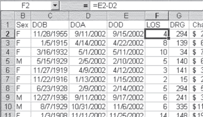
Figure 3.17 Calculation of length of stay
Calculating Age at Admission: Using the =YEARFRAC() Function
Calculation of age at admission by subtracting the date of birth from the date of admission would work, in general, but it would be a little more complicated. First, it would be necessary to make the subtraction, and then convert the resulting age in days from a date format to general format. Finally, it would be necessary to divide the resulting age in days by 365 (or 365.25, allowing for leap years). This would still not give exactly the right age in years and fractions of years, because the number of leap years one has lived through will not always be exactly one-fourth of the years lived. An easier way to find the age is to use the Excel function =YEARFRAC(), which will give the number of years and fractions of years between two dates.
The use of =YEARFRAC() is shown in Figure 3.18. A new column has been inserted between DOB and DOA and labeled Age. Age has been calculated as is shown in the formula line of the spreadsheet. It does not matter in what order the two columns are referenced in the =YEARFRAC() function—the function calculates the number of years between the two dates in either order. An additional function is included in the calculation of age and shows how function statements in Excel can be used together to accomplish a desired data goal. The function =TRUNC() truncates (i.e., cuts off) a number at a specified number of decimal digits. If no number of decimal digits is specified (as in this case), the number is assumed to be zero. Unless the person we are referring to is a child, we cease to refer to people as being a certain number of years old and fractions of years; we refer to them only as the number of years they have attained. So even though the second person on the list (who was born on January 5, 1915, and entered the hospital on April 14, 2002) was actually 87.332 years old at the time of admission, we would refer to her as being 87 years old.
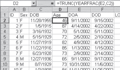
Figure 3.18 Calculation of age
Table 3.1, Table 3.2, and Table 3.3 illustrate the Excel formulas associated with the aforementioned operations.
Table 3.1 Formula for Figure 3.17
| Cell | Formula | Action |
| F2 | =E2-D2 |
Copy cell down to F101 |
Table 3.2 Formula for Figure 3.18
| Cell | Formula | Action |
| D2 | =TRUNC(YEARFRAC(E2,C2)) |
Copy cell down to D101 |
Table 3.3 Formula for Figure 3.19
| Cell | Formula | Action |
| C2 | =IF(B25“F”,1,0) |
Copy cell down to C101 |
Inserting a New Worksheet in a Current Workbook
Now that the age at admission and length of stay have been calculated, it is reasonable to assume that we will not need DOB, DOA, or DOD (date of birth, date of admission, and date of discharge, respectively) any further in our data analysis. So we can now create a spreadsheet that does not include these variables. To do this, we insert a new spreadsheet in the existing Excel workbook by using the Insert ⇨ Sheet option from the Cells menu in the Home ribbon. We then highlight the entire original worksheet (containing the data as originally imported to Excel). This is accomplished by right-clicking the box in the extreme upper left-hand corner of the spreadsheet (the intersection of the letters designating the columns and the numbers designating the rows) and right-click ⇨ Copy. We then move to the new spreadsheet (which is probably labeled “Sheet1”) and left-click in cell A1. Finally, we right-click ⇨ Paste. The entire data set will now be copied to the new spreadsheet.
Having copied the data set to the new spreadsheet, we can now delete the columns DOB, DOA, and DOD. But before we do that, it is necessary to convert the two variables—Age and LOS—from formulas dependent on DOB, DOA, and DOD to actual numbers. To do this, first highlight the entire Age column, and while the column is highlighted right-click and select Copy, then right-click the column again and select Paste Special ⇨Values. This will change the entries in the Age column from a formula dependent on DOB and DOA to actual numbers. Repeat the process for LOS. Now, finally, you can delete DOB, DOA, and DOD by clicking the appropriate column letter (C for DOB in Figure 3.18) and selecting Edit ⇨ Delete.
Transforming Categorical Variables into Numerical Variables
One last data modification should be discussed before we leave the topic of importing data and making them ready for analysis. This is the transformation of categorical variables to numeric variables. Certain data analysis techniques to be discussed later in the book—such as cross-tabulations and chi-square statistics, t tests, and analysis of variance—can accept categorical variables—in the form, for example, of sex as “F” or “M”. Other techniques, particularly regression, cannot accept categorical variables. But a variable such as sex can be included as an independent variable in regression if it is recoded as what is called a dummy variable. A dummy variable is one that takes on two values (as does sex) but is coded 1 for one of the values and 0 for the other.
The result of the import process with the data modified for analysis might be as shown in Figure 3.19. The figure shows Sex1 as modified to a 1/0 variable (with the =IF() statement that produces that change shown in the formula bar). It also shows the ID number and the other variables—Sex, Age, LOS, MS-DRG, Charges, Medicare (payments), Diag (diagnosis), and ICD-9. This working file no longer contains any dates. But if the dates become important at some time during the analysis, it will always be possible to recover them from the original imported worksheet by matching the ID numbers on both worksheets.
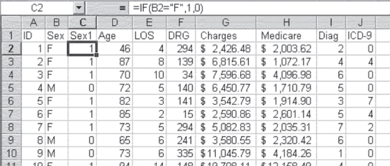
Figure 3.19 Imported file ready for analysis
3.4 Missing Data
One thing we have not yet discussed in regard to the use of data—either collected by the investigator or taken from an existing source—is missing data. The term “missing data” refers to the situation in which some of the observations have no data at all for some or all of the variables under study. In the example given in Section 3.3, the missing data issue was not considered because it was known at the outset that no data were missing. But in most real applications, it is likely that some of the observations will be missing some data. The question then is what to do about this.
First, it is important to recognize that virtually all statistical techniques assume complete data. If one wished to use a statistic to determine, for example, if males had greater or lesser hospital charges than females, based on the data discussed in the previous section, it would be assumed that complete data were available for sex and hospital charges for all 100 observations. But let us now assume that complete data were not available for all 100 observations. Let us assume that some of the data for charges are missing—specifically, that there are no charge data for 9 of the 100 observations. How might we deal with that situation?
Remedy for Missing Data: Case Deletion
The simplest way to deal with the missing charges in this case would be to delete those observations from the data set and base the analysis on 91 rather than 100 observations. There are difficulties with this strategy, however. The first and, in this case, the least important is that dropping the observations with no charge data from the data set reduces the number of observations under consideration. Consequently, the likelihood of finding a statistically significant difference between males and females, if one exists, is also reduced. In general, the more observations one has made, the more likely it is that statistical significance could be found. But going from 100 to 91 cases is likely to have little effect on statistical outcomes. The decrease is a proportionally small one in an already relatively large number for statistical purposes. However, going from 100 cases to 30 or from 30 cases to 20 would have a substantial effect on the ability to find statistically significant results.
Dropping observations can become even more of a problem if there are missing values in more than one of the variables that are to be considered in the statistical analysis. Perhaps there might be nine missing values for charges and five for sex. Unless all the missing values for sex are also missing for charges, there will be more than nine total cases with missing values. All hypothesis testing requires at least two variables, so the number of nonoverlapping missing values in the two variables will determine the number of cases without data. In regression analysis a number of variables may be involved. The total number of missing values will be the total of nonoverlapping missing values for all variables. In some cases, this will act to reduce the total data set to unacceptable levels. In such a case, there are two strategies. The first is to try to go back to the original source to obtain data for the missing values. But this is often impossible.
Remedy for Missing Data: Imputation
The second strategy is to impute—or “fill in”—missing values. There are a number of ways that this may be done, none of which gets high marks from statisticians but which are nevertheless used. The simplest and least time-consuming is to use the mean of the available data to fill in the missing values. So if there are 9 missing values for charges and the mean value for charge for the 91 other observations is $5,676.24, then that value could be assigned to the observations with missing values. There are a number of other strategies, such as using the median or a regression model, that can be used to assign values to missing data. All of these techniques provide somewhat more sophisticated ways of assigning values than does using the simple mean but do require increasingly complex steps. In general, this text will not cover these techniques in any detail.
There is a significant problem with assigning any type of imputed value to data that are missing. Regardless of how it is done, assigning a value to a missing data element will inevitably reduce the variance in that variable. In addition, imputation will be more likely to produce statistically significant results than if the missing values were simply deleted from the data. With this fact in mind, some investigators have used what is known as a Monte Carlo technique to randomly assign values within reasonable ranges to the missing elements. They then observe how these assigned values affect the statistical results over a large number of trials. While this is probably the ideal method for assigning missing values, it is both time-consuming and costly in terms of data analysis.
The bottom line with regard to missing data, then, is that it is probably best to drop cases with missing values. However, this rule of thumb applies only if fewer than 10 percent of cases will be dropped and the overall sample size remains relatively large—for example, over 30. If these circumstances do not prevail, randomly assigning reasonable values to the missing elements is probably the best strategy.