
Chapter 8
Statistical Tests for Categorical Data
As indicated elsewhere in this book, a major part of statistical analysis is the assessment of the independence of two or more variables. The t test assesses the independence of two variables, one measured on a numerical scale and the other measured on a categorical scale that takes only two values. Analysis of variance (ANOVA) assesses the independence of two or more variables. With ANOVA, one variable is measured on a numerical scale and the others are measured on categorical scales that may take on any number of values, although typically the number of values will be limited to fewer than five or six. Regression assesses the independence of two or more variables, all of which can be measured on a numerical scale. The chi-square statistic ![]() is a statistical analysis that can be used to establish the independence of two or more variables, each of which is measured on a categorical scale.
is a statistical analysis that can be used to establish the independence of two or more variables, each of which is measured on a categorical scale.
8.1 Independence of Two Variables
Chapter 5 introduced the subject of independence of two variables. There it was noted that independence could be thought of as mathematical independence or alternatively as statistical independence. This chapter takes up these two topics again, with a more detailed discussion of statistical independence as a way of introducing the chi-square.
Mathematical Independence
The concept of mathematical independence has been discussed previously in Chapter 5. But, to reconsider that discussion here, suppose 100 persons visited the emergency room in the community hospital over the past 24-hour period. Thirty of those people came for true emergencies. Seventy of those people came for some condition that would not be considered a true emergency. Also, 60 of the people came during the day (say, from 6 a.m. to 6 p.m.), whereas the other 40 came at night. The marginal values of this joint distribution are shown in Figure 8.1. Now, if we had no other information about the people who came to the emergency room, how would we expect the people to be distributed in the four internal cells of the table—cells B2:C3? Or, from another perspective, what is the most likely distribution of people in those four cells?
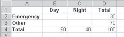
Figure 8.1 Marginal frequencies
After a little thought, most people would conclude that the most likely distribution of people in the four cells—B2:C3—would be as shown in Figure 8.2. It is possible that some people might not even know immediately why they arrived at the frequency distribution shown in cells B2:C3. If questioned, however, they would probably come up with reasoning that involved the idea that, for example, total emergencies are 30 percent of all visits, so emergencies during the day should be 30 percent of all visits that occur during the day. Similarly, emergencies during the night should be 30 percent of all visits that occur during the night. Once either of those decisions is made, the rest of the cells are fixed by the marginal values.
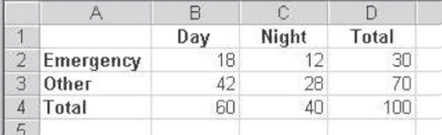
Figure 8.2 Marginal frequencies with most probable internal frequencies
When a person decides that the number of emergencies during the day should be 18, because 18 is 30 percent of 60, all other cells are fixed. If 18 is assigned to the Day/Emergency cell, 12 must be assigned to the Night/Emergency cell, because the sum of the two cells must be 30. Similarly, if 18 is assigned to the Day/Emergency cell, then 42 must be assigned to the Day/Other cell, because the sum of the two cells must be 60. The 28 in the Night/Other cell is fixed in the same way. Because a decision can be made about the number of observations in only one cell of the table, given the marginal totals, a two-by-two table has only one degree of freedom. In general, any r × c (rows × columns) table will have ![]() degrees of freedom. In the table in Figure 8.2, there are two rows and two columns, and thus
degrees of freedom. In the table in Figure 8.2, there are two rows and two columns, and thus ![]() equals 1.
equals 1.
The distribution of observations shown in Figure 8.2 is one that is characterized by mathematical independence. Mathematical independence is defined as a situation in which the marginal probabilities in a table, such as that shown in Figure 8.2, are equal to the conditional probabilities.
Mathematical independence is when marginal probabilities equal conditional probabilities in a joint probability table.
As we saw in Chapter 5, marginal probabilities are just the probabilities associated with the frequency distribution of a single variable. The table in Figure 8.2 has two marginal probabilities, one for the distribution of coming during the day or night, and one for the distribution of coming for an emergency or for another reason. Again, as seen in Chapter 5, a conditional probability for this example could be defined as a patient coming in for an emergency on the condition that the person came during the day.
Marginal and Conditional Probabilities: Link to Mathematical Independence
Figure 8.3 shows the marginal probabilities of a person coming for an emergency or coming for another reason as 0.3(30/100) and 0.7(70/100). Figure 8.3 also shows the conditional probabilities of a person coming for an emergency on the condition that (or given that) one came during the day—or during the night. For example, the conditional probability of a person coming for an emergency, given that one came during the day, is 0.3(18/60). In turn, the conditional probability of a person coming for another reason during the day is 0.7(42/60). If we designate the marginal probability of a person coming for an emergency as ![]() and the conditional probability of a person coming for an emergency, given that one came during the day, as
and the conditional probability of a person coming for an emergency, given that one came during the day, as ![]() , then mathematical independence is defined as
, then mathematical independence is defined as ![]() . The tables shown in Figure 8.2 and Figure 8.3 have only one degree of freedom. Therefore, finding that any one of the conditional probabilities in the table equals any one of the marginal probabilities is equivalent to finding all conditional probabilities equivalent to all corresponding marginal probabilities.
. The tables shown in Figure 8.2 and Figure 8.3 have only one degree of freedom. Therefore, finding that any one of the conditional probabilities in the table equals any one of the marginal probabilities is equivalent to finding all conditional probabilities equivalent to all corresponding marginal probabilities.

Figure 8.3 Marginal and conditional probabilities
It should be clear that this analysis has examined conditional and marginal probabilities in only one direction—by columns. We could equally well have looked at the marginal probability of a person coming during the day p(D) or during the night ![]() . Take a look again at the example table in Figure 8.2. For example, the probability of a person coming during the day p(D) is exactly equal to the probability of a person coming during the day, given that one came for an emergency
. Take a look again at the example table in Figure 8.2. For example, the probability of a person coming during the day p(D) is exactly equal to the probability of a person coming during the day, given that one came for an emergency ![]() . In most cases, though, it is conventional to examine conditional probabilities by columns rather than by rows.
. In most cases, though, it is conventional to examine conditional probabilities by columns rather than by rows.
As indicated here, the definition of mathematical independence for two categorical variables is that the marginal and corresponding conditional probabilities are equal. For a two-by-two table, it is necessary to examine only one conditional probability to make this determination. In a larger table, however, it may be necessary to examine more than one conditional probability to ensure mathematical independence. In general, it will be necessary to look at as many conditional probabilities as there are degrees of freedom in the table before declaring mathematical independence.
Statistical Independence of Two Variables
Before proceeding to discuss statistical independence of two variables, it is important to be sure that what was discussed in the first subsection of Section 8.1 is fully understood. Mathematical independence means that there is no relationship between the time of day (or night) that people arrive at the emergency clinic and whether they come for an emergency. Considered another way, knowing if a person arrived during the day or during the night does not improve any prediction of whether the person came for an emergency.
But consider now that the data examined in the first subsection of Section 8.1 were for only 100 emergency room visits. These visits might be chosen at random, or they might represent a single day's visits or several days' visits. But even if time of day is mathematically independent of arrival for an emergency, we might not always find the results we did. If we had examined a different sample—a larger or smaller sample, for example, or one taken at a somewhat different time—these differences might have led us to find that the conditional and marginal frequencies were very close but were not exact matches. What, then, might we conclude?
Let us posit that the data in Figure 8.4 represent a sample of 100 emergency room visits. These sample visits were taken from among those visits that occurred in the month following the one in which the data in Figure 8.2 were taken. Cells A1:D4 give the actual frequencies for the 100 visits. These visits are divided, as before, into 30 visits for emergencies and 70 for other reasons, with 60 visits occurring during the day and 40 visits occurring at night. Cells A6:D9 show the conditional and marginal probabilities by columns. Now, the conditional probability, for example, of a person coming for an emergency, given that one came during the day ![]() is given in cell B7. This conditional probability is not exactly the same as the marginal probability of a person coming during the day
is given in cell B7. This conditional probability is not exactly the same as the marginal probability of a person coming during the day ![]() . So one might conclude that the two variables are no longer independent mathematically. However, are they close enough to be considered independent statistically, and what might that mean?
. So one might conclude that the two variables are no longer independent mathematically. However, are they close enough to be considered independent statistically, and what might that mean?
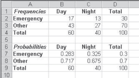
Figure 8.4 Different conditional probabilities
Statistical Independence: The Chi-Square Test
Statistically, if we took many samples of size 100 of people who came to an emergency room, we would expect that the conditional probabilities would not match exactly the marginal probabilities for every sample. This would be true even if the variables, time of arrival, and arrival for an emergency were truly mathematically independent of one another. So we would like to have a statistical test to determine whether the two variables can be considered statistically independent of each other. We would like this test even if the two variables are not considered strictly mathematically independent for every sample we may examine. The test of statistical independence is the chi-square, or ![]() test.
test.
The chi-square test determines if two variables are statistically independent of each other.
The chi-square test is a test of independence between two variables. It is calculated as given in Equation 8.1. In Equation 8.1, r is the number of rows in the table and c is the number of columns. O is the observed frequency in each cell, and E is the expected frequency in the cell. The squared difference between each observed frequency and each expected frequency is divided by the expected frequency. These values are then summed across all r × c cells in the table. The result is the chi-square value. If the chi-square value is greater than some predetermined value, the two variables will be considered statistically independent.
Consider the data shown in cells B2:C3 in Figure 8.4 as the observed values. Based on the conditional probabilities shown in cells B7:C8, we know that the two variables shown in that table are not mathematically independent. But if we calculate the chi-square, will they be found to be statistically independent? To determine this, we need to know the expected values. But what are the expected values? It turns out that the expected values are the values we will expect to get if the marginal probabilities and the conditional probabilities are the same—in other words, what we decided should be the values in cells B2:C3 in Figure 8.2, based on the distributions of the marginal values. Given these expected and marginal values, the calculation of the chi-square statistic for the data shown in cells B2:C3 in Figure 8.4 is shown in Equation 8.2. The calculated chi-square value is 0.1984. The question then would be, what is the likelihood of finding a chi-square value that large if the null hypothesis that arriving for an emergency is independent of time of arrival is actually true?
The =CHIDIST() Function
The probability of a chi-square value as large as 0.1984, given that the null hypothesis of independence is true, is found with the =CHIDIST() function. The =CHIDIST() function takes two arguments: the value of the chi-square statistic and the number of degrees of freedom. The calculation of the =CHIDIST() function shown in Equation 8.3 is 0.656. This value means that there is about a 66 percent probability of finding a chi-square value as large as 0.1984 under the null hypothesis that arrival for an emergency is independent of time of arrival. In general, we would reject the null hypothesis only if the probability of the chi-square value were less than 0.05; so, in this case, we would conclude that the observed frequencies in cells B2:C3 in Figure 8.4 are not different enough from the expected frequencies. In turn, we would say that time of arrival and arrival for an emergency are statistically independent of each other.
The =CHIINV() Function
But how large must a chi-square be before one can conclude that the two events are statistically independent? The value of the chi-square required, referred to as the critical value of the chi-square, can be found using the =CHIINV() function. This function takes two arguments: the probability at which we will reject the null and the degrees of freedom. The critical value for the chi-square for a table with one degree of freedom (any table with two rows and two columns) is given in Equation 8.4. According to that equation, it is necessary to have a chi-square value of at least 3.84 before the null hypothesis of statistical independence is rejected at the 95 percent level of confidence.
The Chi-Square Critical Value
What kind of difference would be necessary between observed and expected values in the table in Figure 8.4 before the critical value of chi-square would be reached? Figure 8.5 shows a template for the calculation of the chi-square statistic. The template also shows one of the smallest differences in the distribution of observed versus expected values that result in a chi-square that exceeds the critical value. Figure 8.5 deserves substantial explanation.
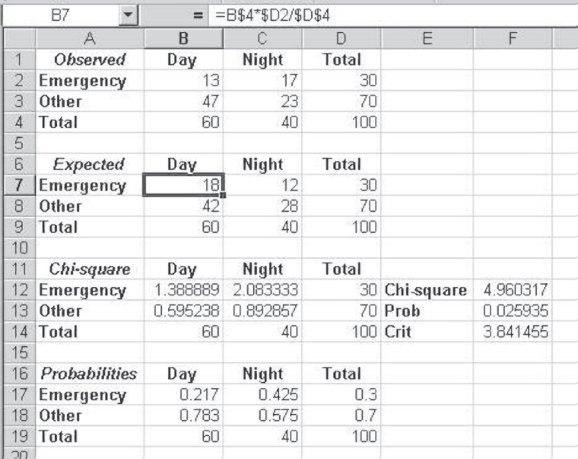
Figure 8.5 Template for the chi-square
First, consider cell B2 of Figure 8.5. The value of 13 in the cell (13 people came for emergencies during the day) is the closest value to the expected (shown in cell B7) that can appear in that cell and produce a chi-square greater than the critical value. Because there is one degree of freedom in this example, 13 in cell B2 fixes all three other cells in B2:C3, given the marginal values in column D and row 4. The expected values for the given marginal values (cells B7:C8) are shown in Figure 8.2, but here, a simple way of calculating those expected values is given. The formula for cell B7 is shown on the formula line above the spreadsheet. The formula uses the $ convention to fix appropriate rows and columns so that it can be copied to all four cells in which expected values are desired. To explain the formula, B$4 fixes the first term in row 4, which allows the formula to be moved to cell B8 without changing the reference to cell B4. $D5 fixes the second term in the equation in column D so that it is possible to move the equation to cell C7 without changing the reference to cell D2. Finally, $D$4 fixes cell D4 so that it is possible to move the equation to any of the cells without changing the reference to cell D4. With this formula in cell B7, it is possible to click the lower right corner of the cell and drag the formula across to cell C7, and then to drag both cells down to row 8. This produces the expected values for the marginal values observed.
The values shown in cells B12:C13 are the calculations of the chi-square statistic. Each cell represents one of the calculations ![]() , shown in Equation 8.1. The chi-square value itself is shown in cell F12 and is the sum of cells B12:C13. The probability of the chi-square value is shown in cell F13 as 0.0259. Because this value is less than 0.05, we would reject the null hypothesis that the two variables—arrival for an emergency and time of arrival—are independent of each other.
, shown in Equation 8.1. The chi-square value itself is shown in cell F12 and is the sum of cells B12:C13. The probability of the chi-square value is shown in cell F13 as 0.0259. Because this value is less than 0.05, we would reject the null hypothesis that the two variables—arrival for an emergency and time of arrival—are independent of each other.
The last table in Figure 8.5 shows the conditional probabilities of reason for arrival, given arrival during the day or during the night. These conditional probabilities show that about 22 percent of the people arriving during the day came for an emergency, whereas about 43 percent of those coming at night came for an emergency. In general, one of the best ways to interpret the results of a chi-square applied to any contingency table is to form the conditional probabilities by columns and interpret them by comparing rows. For our example, compare the conditional probabilities for those who came for an emergency during the day or during the night. This gives a succinct way of describing the differences in the observed values that produce the chi-square value large enough to reject the null hypothesis of independence.
Using the =CHITEST() Function
Microsoft Excel does not include a Data Analysis add-in to do the chi-square test, but it does include a function that will carry out the chi-square analysis. This function is =(). The =CHITEST() function takes two separate arguments: the range represented by the observed data and the range represented by the expected data. The table in Figure 8.6 reproduces the observed and expected frequencies from Figure 8.5, but it now shows the calculation of the =CHITEST() function, in cell D11. The formula line in Figure 8.6 shows the two ranges B2:C3 and B7:C8, which are included as arguments of the =CHITEST() function. The =CHITEST() function produces not the chi-square value but the probability of finding that value, given the null hypothesis of independence. The actual chi-square value can be reproduced by using the =CHIINV() function with the value of the probability and one degree of freedom. This reproduced chi-square value is shown in cell D12. The =CHIINV() function will not always reproduce the chi-square value, however. If the probability of the chi-square is less than 3.0E-7, the =CHIINV() function returns #NUM!.
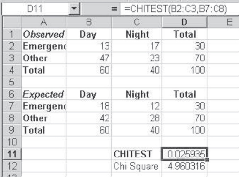
Figure 8.6 The =CHITEST function
The Chi-Square and Type I and Type II Errors
Chapter 7 introduced the notion of Type I and Type II errors with regard to the t distribution. A few comments should be made about Type I and Type II errors with regard to the chi-square distribution. The chi-square distribution is not a “normal” distribution as the t distribution is, in the sense that it is symmetrical about some mean value. In fact, the chi-square distribution tends to be heavily skewed to the right. Figure 8.7 shows the chi-square distribution with one degree of freedom. This is the most extremely skewed chi-square distribution. As degrees of freedom increase, the distribution begins to take on a less skewed appearance, and if the degrees of freedom increase to 40 or 50, the distribution begins to look more and more normal. But most chi-square applications, particularly in regard to contingency tables, are limited to degrees of freedom in the range 1 (a two-by-two table) to less than 10 or 12 (a four-by-five table).
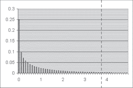
Figure 8.7 The chi-square distribution for one degree of freedom
With one degree of freedom, the point in the distribution at which the null hypothesis of no relationship between two variables (as previously discussed) would be rejected at alpha = 0.05 would be at approximately 3.8 (as shown by the vertical dashed line in the figure). Any chi-square value that resulted in a probability to the right of the dashed line (i.e., any value greater than 3.8) would be expected to occur less than 5 percent of the time when the null hypothesis is true. Thus, any value in that range would lead to the rejection of H0 (no relationship between or independence of the two variables) and the acceptance of the alternative—that the two variables are not independent. The area to the right of the dashed line, then, which is usually set at 0.05, is the area of Type I error, or alpha.
Type I Error
Let us consider the Type I error in another way. In the example analysis shown in Figure 8.5, the expected joint probability “and” for Day and Emergency is 18/100, or 0.18. Because the other probabilities in the table are fixed by 0.18, given the marginal values (the table has one degree of freedom), the expected probabilities for the other three cells are 0.12 for Night and Emergency, 0.42 for Day and Other, and 0.28 for Night and Other. Let's say we generate many samples—say, 1,000 samples of size 100—from a population in which these proportions are true. In turn, the distribution of chi-square values for these samples would be such that approximately 5 percent (about 50 out of the 1,000) would have chi-square values that exceed 3.8. So even though the null hypothesis of independence would be true, there would be some proportion of the samples for which we would reject H0.
Type II Error
But what now of beta or the Type II error? How can we conceive of the Type II error with this same example? To see this, consider the possibility that the true proportion of Day and Emergency visits is not 0.18 but 0.15 in the larger population (the other proportions change at the same time). Let's assume we again took many samples (1,000 samples of size 100) from a population in which the true proportion of Day and Emergency was 0.15. In turn, we would discover that about 70 percent of these samples had values of the chi-square that did not exceed 3.8 (the 0.05 level of significance). Thus, in the case of a true proportion for Day and Emergency of 0.15, we have about a 70 percent chance of making the Type II error (accepting the null hypothesis of independence, or Day and Emergency equals 0.18) when it is false.
In fact, one may ask, what if there were an even greater variation from 0.18? Suppose the actual probability of Day and Emergency in the population is 0.11. Do we now have any chance of making the Type II error? The answer is yes. Suppose we took many samples (1,000 samples of size 100) from a population in which the true proportion of Day and Emergency was 0.11. We would discover that about 10 percent of those samples would have values less than 3.8; so, in this case, we would have about a 10 percent chance of making the Type II error.
As with the Type II error associated with a normal or t distribution, we can reduce the Type II error associated with the chi-square by increasing the sample size. Again, suppose we were to take a large number of samples of a larger size (1,000 samples of size 200) from a population in which the true proportion of Day and Emergency was 0.15. We would discover that only about 50 percent of the samples would lead us to falsely accept H0 (Type II error), whereas the other 50 percent would lead us correctly to reject H0. The larger the sample we take, the lower the level of beta will be for any given divergence of the true value from that hypothesized by H0.
8.2 Examples of Chi-Square Analyses
Thus far the discussion has focused solely on contingency tables with one degree of freedom (two-by-two tables). This section will consider several examples of chi-square calculations taken from examples that have appeared in various journals and includes further discussion of not only two-by-two contingency tables but also larger contingency tables.
An Example of a Two-by-Two Table
To better understand the chi-square test and its interpretation, consider the example shown in Figure 8.8. That figure shows data taken from an article by Halpern et al. ([2001]), and the data shown in the table were taken from the second table in the article (p. 1682). Figure 8.8 contains data to address the question of whether an adolescent has experienced either physical or psychological violence from a partner in an opposite-sex romantic relationship. The supposition is that the violence is independent of whether the respondent is male or female. The implied null hypothesis is independence; the implied alternative is nonindependence.
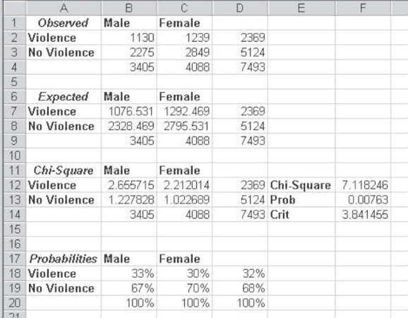
Figure 8.8 Example from the Halpern et al. ([2001]) article
In Figure 8.8, cells A1:D4 show the observed cell values and marginal values. Cells A6:D9 show the expected values based on the calculations shown in cell B7 in Figure 8.6. Cells A11:D14 show the calculation of the chi-square values for each cell, and cell F12 shows the total chi-square value. The probability of this chi-square value under the null hypothesis of independence is shown in cell F13 as 0.0076. Because this value is less than 0.05, we reject the null hypothesis of independence and conclude that experiencing violence is not independent of sex.
Interpreting the Chi-Square Statistic: Statistical versus Practical Significance
Saying that experiencing violence is not independent of sex implies that either male adolescents or female adolescents are more likely than the other gender to experience violence in an opposite-sex romantic relationship. But by looking at the observed values in cells A1:D4, it is difficult to tell which sex is more likely to experience such violence. Consequently, the easiest way to interpret the results of a chi-square test is by looking at the conditional probabilities of experiencing violence. Cells A17:D20 show the conditional probabilities of having experienced violence, given sexual identity. Perhaps somewhat surprisingly, 33 percent of males said that they had experienced violence, whereas 30 percent of females said the same. These percentage differences are not large, but the fact that there are 7,493 respondents in the study gives this relatively small percentage difference statistical significance.
Having seen the results from Figure 8.8, it is useful to say a few words about the difference between statistical significance and practical significance. The notion of statistical significance is associated with the rejection of the null hypothesis, whether that hypothesis is explicit or implied. So, in the case of the data examined in Figure 8.8, “statistical significance” refers to the fact that the chi-square value is large enough to reject the null hypothesis. But “practical significance” refers to the importance of a result found in a statistical test. Because the number of respondents is relatively large, as shown in Figure 8.8, a relatively small percentage difference results in statistical significance. Whether this relatively small percentage difference has practical significance is not a question that can be addressed by statistics. It is a question that can be addressed only by knowledge of the subject, experience, and understanding. Consequently, statistics can address statistical questions, but the value placed on the results of statistical analysis remains with the observer, who must assess the importance of these results.
An Example of an n-by-Two Table from the Literature
The extension of the chi-square statistic to tables with more than four cells is direct. The original data reported in the article referenced for Figure 8.8 were presented for the experiencing of physical violence, psychological violence, or no violence. The tables in Figure 8.9 show the data in both categories of violence and no violence. Cells A1:D5 are the observed values for the data, whereas cells A7:D11 are the expected values. Again, the expected values are calculated by multiplying the row total for each cell times the column total for the cell and dividing by the grand total. The formula used and replicated by dragging to each cell, B8:C10, is shown in the formula bar in Figure 8.9. Cells B14:C16 are the chi-square values for each individual cell, and the overall chi-square value is shown in cell F14. The probability of the chi-square value in cell F14, under the implied null hypothesis of independence, is given in cell F15. The value in cell F15 is now determined with =CHIDIST() with two degrees of freedom. The critical value for a chi-square with two degrees of freedom is given in cell F16.
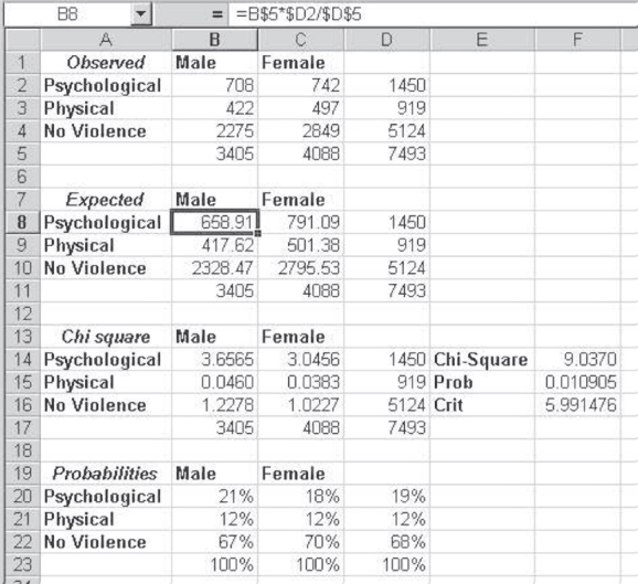
Figure 8.9 An n-by-two chi-square
Notice that the critical value is 5.99, which is very close to six. The data being analyzed in Figure 8.9 are presented in a three-by-two table. Each table contains six internal cells. The data analyzed in Figure 8.8 were in a two-by-two table. A two-by-two table has four cells, and the critical value was 3.8. A three-by-two table has six cells, and the critical value is about 6. In general, one can be fairly certain that if the chi-square value is as large as the number of cells in a table, it is likely that the null hypothesis of independence will be rejected at the 0.05 level.
In general, if the chi-square value is as large as the number of cells in the contingency table, it is likely that the null hypothesis of independence will be rejected at the 5 percent level.
Again, the question of how the interpretation of the data is to be made arises. The interpretation is best based on the conditional probabilities of experiencing different types of violence or no violence, given that the recipient is male or female. Cells B20:C22 show these differences. The major difference in the experiencing of violence between males and females is that 21 percent of males reported experiencing psychological violence, whereas 18 percent of females reported such violence. There is no difference in the percentages for physical violence.
An Example of a Two-by-n Table from the Literature
An example of a two-by-n variable is also available from the literature. The data in Figure 8.10 came from a study of 3,158 women in the Sudan with at least one child. The study was reported in Studies in Family Planning (1992). The women were asked if they wanted another child. Their answers were tabulated with the number of children they currently had in categories from one to five and six or more. The observed frequencies are given in cells A1:H4. The expected frequencies are given in cells A6:H9. The formula for the calculation of expected frequencies is shown for cell B7 in the formula line at the top of the figure. The chi-square values for the individual cells are shown in cells A11:H14, and the overall chi-square, 531.72, is given in cell J12. The probability of the chi-square is given in cell J13. You should recognize that the chi-square value in this case is very large and the probability is very small. Because the number of cells in the table is 12, the critical value of the chi-square is about 12 (actually 11.07). Any value of the chi-square larger than this would lead us to reject the implied null hypothesis of independence between the number of children and the desire for an additional child. In short, we reject that implied null.
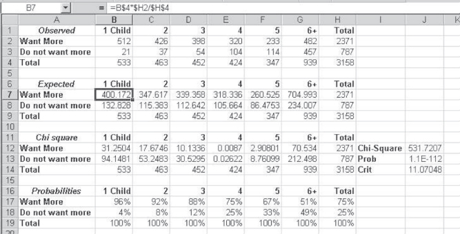
Figure 8.10 Number of children and desire for more
The conditional probabilities of wanting an additional child, given the number of children a woman already has, are shown in cells A16:H19. Ninety-six percent of women with only one child want an additional child. Only 51 percent of women with six or more children want an additional child. Between these two extremes there is a monotonic decrease in the percentage of women who want another child. The conclusion is quite clear: Among these women from the Sudan, the more children a woman has, the less likely she is to desire an additional child. Although this is not unexpected, the data from this study confirm the expectation.
An n-by-n Example from the Literature
The extension of the chi-square statistic from n-by-two or two-by-n to n-by-n tables is also direct. Consider, for example, the data shown in Figure 8.11. These data represent the results of a study carried out by Brook and Appel ([1973]) on the assessment of the quality of medical care. Each of three physicians reviewed 296 case records for patients who had been treated for urinary tract infection (UTI), hypertension (Hyper), or ulcer. The treatment of the case was judged adequate or inadequate by each of the three physicians. On the adequacy dimension the data are displayed in three categories: judged adequate by two or three physicians (Adequate by 2+), judged adequate by one (Adequate by 1), or judged adequate by none (Adequate by 0).
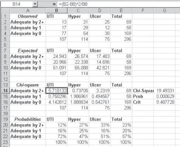
Figure 8.11 Adequacy of treatment of three conditions
Cells A1:E5 show the observed data for the 296 cases. Cells A6:E11 show the expected values for each of the cells by the convention column total × row total/grand total. The chi-square calculations for each individual cell are shown in cells A13:E17, and the overall chi-square value of 19.49 is shown in cell G14. The actual probability of obtaining a chi-square value that large under the null hypothesis that adequacy of treatment is independent of diagnosis is given in cell G15 as 0.0006, or 6 times out of 10,000. Because the probability is so small, we conclude that we must reject the null hypothesis, which is equivalent to saying that judged adequacy of treatment depends on the initial diagnosis.
To see which diagnosis is more likely to be judged to be treated adequately, it is useful to form the table of conditional probabilities shown in cells A19:E23. Here it can be seen that 12 percent of UTI cases are judged adequately treated by two or three physicians, whereas 27 and 33 percent of hypertension and ulcer, respectively, are similarly judged. However, 72 percent of UTI cases are judged adequately treated by not a single one of the three physicians. Clearly, the dependence between judgment of adequacy and diagnosis rests primarily in the difference between UTI cases and the other two.
8.3 Small Expected Values in Cells
The use of the chi-square statistic assumes relatively little about the data. There is no underlying assumption, for example, that the data need be normally distributed. Any data in a contingency table will be acceptable. There is one limitation, however, about the magnitude of the expected value in any cell in the contingency table. In general, small expected values in any table cell tend to inflate the value of the chi-square and increase the likelihood of rejecting the null hypothesis when it should not be rejected. There are several ways of dealing with this possibility, and these alternatives depend, in part, on the number of cells in a table.
Small Expected Values When df > 1
If the expected value in any cell of a two-by-two table is less than about 10, one way of dealing with the small expected values is to apply what is known as Yates's correction. Yates's correction is applied using the formula shown in Equation 8.5, which indicates that the absolute value of the difference between the observed and expected frequencies is reduced by 0.5 before the value is squared. To see how the application of this equation works, consider the example shown in Figure 8.12.
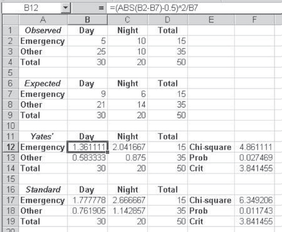
Figure 8.12 Yates's correction
Figure 8.12 shows data comparable to that in Figure 8.2, except that in the case of Figure 8.12 there are only 50 observations rather than 100. The consequence of this difference, given the same marginal probabilities, is that the expected values for cells B7 and C7 are less than 10. In this case, the chi-square formula given in Equation 8.1 is not strictly appropriate, because it produces a chi-square value larger than it should be. For the observed data seen in cells A1:D4, the chi-square using Yates's correction (Equation 8.5) is shown in cells A11:F14. The comparison chi-square using the standard formula (Equation 8.1) is shown in cells A16:F19. Although the decision one would reach does not differ in either of these computations, it can be seen that the Yates's corrected chi-square is a more conservative test. It is less likely than the standard formula to result in a rejection of the null hypothesis when expected cell values are small.
When expected cell values fall below 5, Yates's correction is also no longer considered appropriate. In such a case, the statistical test recommended is the Fisher exact test. The calculation of the Fisher exact test, although not difficult using Excel, is complicated and difficult to understand, and so it is not presented here. In general, the decision reached by the Fisher exact method, although statistically correct, will not be different from the decision reached using either the chi-square or the chi-square with Yates's correction. One reasonable approach to the issue of very small cells would be to base the decision on the probabilities derived from the Yates's correction. This will be, in general, more conservative than the Fisher exact test, in that the null hypothesis of independence is slightly less likely to be rejected. But, at the same time, the probability of making the Type I error will not be greater than the probability level that has been set.
Small Expected Values When df > 1
When degrees of freedom are greater than one, or in other words tables are larger than two rows by two columns, there is no equivalent to Yates's correction or the Fisher exact method. In such tables, two strategies might be used. One is to try to increase the number of observations in general, so that the expected cell frequencies in all cells are at least 5 and preferably 10. Another strategy is to collapse cells where doing so might make logical sense in order to increase the expected values in cells. To illustrate this latter approach, consider again the data shown in Figure 8.11. Those data were originally given in the form of the table shown in Figure 8.13. The two rows adequate by 3 and adequate by 2 were collapsed into a single row, adequate by ![]() , to avoid the small expected value in cell M9.
, to avoid the small expected value in cell M9.
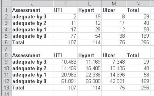
Figure 8.13 Small expected values in df > 1
It is worth noting that in the case of the data shown in Figure 8.13, numerous researchers would not bother to collapse the two rows adequate by 3 and adequate by 2. This could be considered to be justified because the expected value in cell M9 is not all that small and there is only one such cell smaller than 10. This logic could change had there been several cells with expected values smaller than 10, or if any of the cells had been less than 5. Collapsing the cells or increasing the overall number of observations in the study would have been most advisable from the standpoint of the appropriateness of the chi-square value.