Chapter 10
Analysis of Variance
Chapter 1 introduced several different questions that could be addressed using statistics. One of these was the question of whether eight hospitals in a hospital alliance differed from one another in length of stay, readmission rates, or cost per case. If we were interested in whether just two of the hospitals differed from one another, we could use a t test. As presented earlier, a t test is a test of whether a numerical variable is independent of a categorical variable that takes on only two values. But in this case, the question is whether a numerical variable is independent of a categorical variable that may take on more than two values—here, eight. One statistical test that can be used to determine if a numerical variable is independent of a multilevel categorical variable is analysis of variance, commonly referred to as ANOVA.
10.1 One-Way Analysis of Variance
A one-way analysis of variance is a technique used to compare means of two samples that can be used only for numerical data.
To simplify the example somewhat, we are going to assume that there are only four hospitals in the alliance. However, it should be noted that the principles would be the same for essentially any number of hospitals being observed. Now if we were to examine the question of whether the four hospitals in the hospital alliance differed on the measures of length of stay, readmission rates, or cost per case, we could use one-way analysis of variance. With length of stay, it is possible that we could obtain all the data for each hospital—for example, for the last month or the last year or the last 10 years. This would be an overwhelming amount of data for an example. For readmission rates, we might be able to get all the data for each hospital as long as the readmission was to the same hospital. Coordinating among hospitals in the alliance or with hospitals outside the alliance would be more difficult. So, in the case of length of stay, we might have too much information, and in the case of readmissions, we might have too little. But with regard to cost per case, we might be just right.
Recall that Chapter 7 discussed the likelihood that cost per case is not really known. But it might be possible for a hospital's chief financial officer, for example, to get a good idea of cost per case for a relatively small random sample of hospital discharges. Let us assume that the head of the hospital alliance has reached an agreement with the hospital CFOs. The hospital alliance will each select a random sample of 30 hospital discharges. In turn, using accounting procedures commonly agreed to, they will determine the cost of each of the 30 discharges for each hospital. When they have finished, they will have a cost figure assigned to each discharge. Before we discuss these specific hospital discharges, it will be useful to spend a little time discussing what analysis of variance means in relation to the t test. Let's discuss this with the average cost of hospital discharges as the subject.
Analysis of Variance: Relation to t Tests
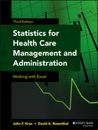
If we were examining only the average cost of the discharges from two hospitals, what we would actually be examining with a t test could be characterized as shown in Figure 10.1, which shows two distributions: one around a mean discharge cost of $5,700 and one around a mean discharge cost of $9,400. For the sake of this discussion, each of these distributions is assumed to have a standard error of $800. The t test is a test of whether the two mean values, given their respective distributions, can be thought of as being different from each other. In the case of Figure 10.1, the t test would definitely indicate that these two means are different. More specifically, the mean discharge cost is not independent of the hospital of discharge because the two distributions overlap only slightly.
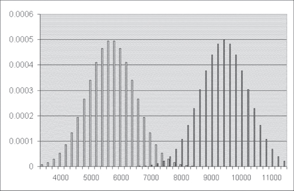
Figure 10.1 Average cost distribution for two hospitals
Analysis of variance examines essentially the same question, but for more than two levels of a categorical variable. Consider, for example, the graph shown in Figure 10.2, which shows the distribution around the average discharge cost for four hospitals, the lowest being $5,700 and then rising to $6,300, $6,600, and finally $9,400. All of these hospitals are assumed to have equal standard errors of $800. Analysis of variance addresses the question of whether the average cost per discharge of any of the four hospitals can be seen as being different from any of the others. In the case of these four hospitals, it is quite likely that analysis of variance would show that their average costs per discharge are not all the same. This is apparent, as there is little overlap between the distribution of the hospital with the highest average costs and that of the other three hospitals.
Figure 10.2 Average cost distribution for four hospitals
Equations for One-Way Analysis of Variance
So how is analysis of variance carried out? Analysis of variance depends on two pieces of information. The first of these is the between group variance, sometimes referred to as the explained variance. The between group variance is associated with the differences between the groups—in this case, four different hospitals. The second is the within group variance, often referred to as the error variance. The within group variance is a measure of the difference between the observations within the groups—in this case, each individual hospital—and cannot be accounted for by any information available to the analysis.
Between Group Variance: SSB
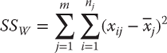
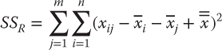
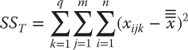
The between group variance (designated SSB) is calculated as shown in Equation 10.1, which indicates that the between group variance requires that the grand mean for all observations—in this case, the 120 observations from all four hospitals—be subtracted from the mean for each group. In turn, this difference is then squared. The result for each hospital is then multiplied by the sample size from each hospital and summed across all m hospitals—here, four hospitals.
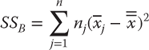
where m represents the number of separate groups, nj designates the number of observations in each group, xj designates the sample mean for group j, and ![]() designates the mean for all observations across all groups.
designates the mean for all observations across all groups.
Between Group Variance: SSW
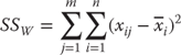
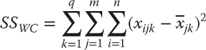
The within group variance (designated SSW) is calculated as shown in Equation 10.2, which says that the mean cost for the sample from each hospital is subtracted from each separate observation for a specific hospital and then squared. This result is summed over all observations for each group—hospital—and these results are then summed across all hospitals.
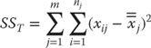
Although the between group variance SSB and the within group variance SSW are all that are required for the calculation of the analysis of variance, it is useful to know the formula for the total variance (SST). This is useful because SST = SSB + SSW. If there is ever any doubt about whether your calculations have been carried out correctly, it is possible to calculate all three values and be sure that, in fact, SST = SSB + SSW. The formula for SST is shown in Equation 10.3, which indicates that the grand mean for all observations is subtracted from each individual observation and that each of these results is squared. Then these are summed across all observations in each group and then across all groups.
Calculation of One-Way Analysis of Variance for Four Hospitals
Now we'll look at an example of the analysis of variance calculation, using Microsoft Excel. Let's call the four hospitals in the alliance Albemarle Community, Beaufort Municipal, Catawba County, and Dare Regional. The CFOs of four hospitals in the alliance have agreed to select a random sample of 30 discharges and determine actual costs for these discharges. The data they generated are contained in the file Chpt 10–1.xls, and the first 14 observations are shown in Figure 10.3.
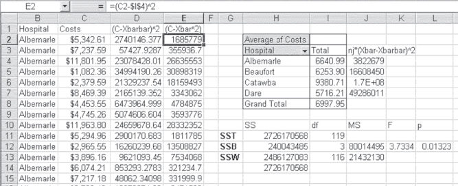
Figure 10.3 Analysis of variance for four hospitals
As should be clear from Figure 10.3, all of the first cost records (column C) are for a single hospital: Albemarle Community. The cost data for the other three hospitals are contained in rows 31 to 121. A discussion of the presentation in Figure 10.3 should begin with the pivot table in cells H2:I8. This pivot table shows the average cost for each hospital (cells I4:I7) and for all hospitals taken together (cell I8). The average cost per hospital and for all hospitals is obtained by changing Sum to Average in the Layout window for the pivot table (see Figure 4.25).
Computation of SST in Excel
The computation of SST is contained in column D, which is labeled (C-Xbarbar)^2. This indicates that the overall average (designated ![]() in Equations 10.1 and 10.3 and given as Xbarbar in the figure) is subtracted from the discharge cost figure in column C and then squared. The value of Xbarbar is taken from cell I8 in the pivot table. Each of the values in column D is summed in cell H11 and labeled SST in cell G11. The formula for cell H11 is =
in Equations 10.1 and 10.3 and given as Xbarbar in the figure) is subtracted from the discharge cost figure in column C and then squared. The value of Xbarbar is taken from cell I8 in the pivot table. Each of the values in column D is summed in cell H11 and labeled SST in cell G11. The formula for cell H11 is =SUM(D2:D121). Although SST is not part of the test of whether the four hospitals differ from one another, it is an important check of MSB, the mean square error between groups, and MSW, the mean square error within groups.
The between group variance, SSB, is calculated in cells J4:J7 and summed in cell H12. The values in cells J4:J7 are calculated by subtracting the grand total mean in cell I8 from each of the hospital means in cells I4:I7, squaring the result, and multiplying by the number of observations for each hospital—in this case, 30 for each. The result is then summed in cell H12, the formula for which is =SUM(J4:J7). Note that the 1.7E+08 in cell J6 is simply Excel's way of designating a number too large to display in the cell.
The within group variance, SSW, is calculated in column E and summed in cell H13. The formulas used by Excel to calculate the values in column E are shown in the formula bar. The individual hospital averages, given in cells I4:I7, are subtracted from the cost of the discharges for each hospital and squared to get the values in column E. The first 30 values in column E use the average for Albemarle Community, given in cell I4; the next 30 use the average for Beaufort Municipal, given in cell I5; and so on for the other two hospitals. The results of all these operations are summed in cell H13, labeled SSW. The formula for cell H13 is =SUM(E2:E121). The value shown in cell H14 is the sum of cells H12 and H13, to verify that, indeed, SSB and SSW actually sum to SST. Table 10.1 displays the associated formulas for the computation of SST in Excel.
Table 10.1 Formulas for Figure 10.3
| Cell or Column | Formula | Action/Note |
| D Column | =(C2–$I$8)2 |
Copied to cell D121 |
| E Column | =(C2–$I$4)2 |
For column B cells containing Albemarle |
=(C2–$I$5)2 |
For column B cells containing Beaufort | |
=(C2–$I$6)2 |
For column B cells containing Catawba | |
=(C2–$I$7)2 |
For column B cells containing Dare | |
| H11 | =SUM(D2:D121) |
|
| J4 | =30*(I4–$I$8)2 |
|
| J5 | =30*(I5–$I$8)2 |
|
| J6 | =30*(I6–$I$8)2 |
|
| J7 | =30*(I7–$I$8)2 |
|
| H12 | =SUM(J4:J7) |
|
| H13 | =SUM(E2:E121) |
|
| H14 | =SUM(H11:H13) |
|
| I11 | =COUNT(C2:C121)–1 |
|
| I12 | =4–1 |
|
| I13 | =I11–I12 |
|
| J12 | =H12/I12 |
|
| J13 | =H13/I13 |
|
| K12 | =J12/J13 |
|
| L12 | =FDIST(K112,I12,I13) |
The F Test for Differences in ANOVA
The test of whether hospital costs (a numerical variable) are independent of hospitals (a categorical variable that takes on four values) is an F test. The question raised is whether the variance of the numerical variable associated with a categorical variable that took on only two values was different for the two levels of the categorical variable.
You will recall that if it was, then the t test assuming equal variance was not strictly appropriate. Take note, though, that in the case of equal-sized groups for each level of the categorical variable, it was probably adequate.
The F test is a statistical test in which the test statistic has an F distribution if the null hypothesis is true.
The use of the F test to determine the independence of hospital costs and hospital categories is similarly a test of variances. But, in this case, it is a test of whether the between group variance—the variance that can be attributed to the differences between the hospitals—is large relative to the within group variance. The within group variance is the variance that cannot be explained by information about the different hospitals. It is considered error variance. But the F test of whether the between group variance is large relative to the within group variance is not directly a test of the relative size of SSB and SSW. If there are m different groups (in this case, four hospitals), then there are m − 1 degrees of freedom in SSB. If there are nj separate observations in each group (in this case, 30 cost figures for each hospital, although the number could be different for each hospital), then there are n1 − 1 + n2 − 1 + . . . nj − 1 degrees of freedom in SSW. In Figure 10.3, the degrees of freedom for SSB and SSW are shown in cells I12 and I13, respectively. The degrees of freedom for SST are given in cell I11. It is the total number of observations minus one, and it should always equal the sum of the degrees of freedom for SSB and SSW.
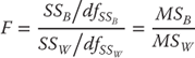
Cells J12 and J13 in Figure 10.3 show what are known as the mean square between groups and the mean square within groups, respectively. The mean square is found by dividing the between group variance and the within group variance by their respective degrees of freedom. The F test of whether the between group variance is large relative to the within group variance is actually calculated on the mean square values rather than on SSB and SSW. The formula for the F test is shown in Equation 10.4.
The =FDIST() Function
As Equation 10.4 shows, the F test is the mean square between groups divided by the mean square within groups. The result of this operation is shown in cell K12 in Figure 10.3. The value of F is given as 3.7334. Now, of course, there arises the question of whether this F value is large or small. The probability of obtaining an F value as large as 3.7334 can be found with the =FDIST() function. The function takes three arguments: the F value itself and the degrees of freedom in the numerator and in the denominator. The actual probability of this F value is given in cell L12 as 0.01323. The Excel function statement for that value is =FDIST(3.7334,3,116) but in the figure is actually stated as cell references K12, I12, and I13. What the probability value of 0.01323 says is that there is a very low probability of getting an F value as large as 3.7334. Actually, there is only about one time in 100 sets of samples, if cost and hospital are actually independent of each other. In consequence, we would conclude that cost is not independent of the hospitals and that the hospitals do, in fact, differ in their costs.
The Excel Add-In for One-Way Analysis of Variance
Now we can turn to the calculation of analysis of variance by using the Excel ANOVA Single-Factor Data Analysis add-in. The data for the Excel single-factor ANOVA must be arranged differently from the data shown in Figure 10.3. The data must be arranged in columns, each column representing a single group—in this case, a single hospital. The first 14 discharge costs for each of the four hospitals are shown in Figure 10.4, arranged in four columns.
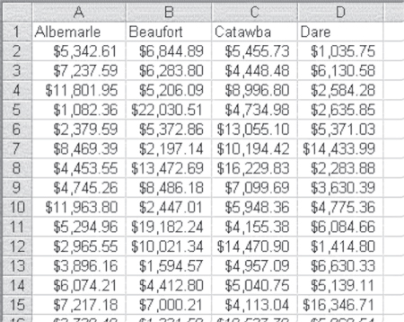
Figure 10.4 Data arrangement for the Excel Single-Factor ANOVA add-in
To access the ANOVA: Single-Factor option in the Data Analysis package within Excel, go to the Data ribbon, in the Analysis group, and click the Data Analysis option. From the Data Analysis menu choose ANOVA: Single-Factor. The dialog box shown in Figure 10.5 prompts you for the same type of information that most data analysis add-in dialogs require. The Input Range is the data to be used in the analysis and includes all cells A1:D31. This includes all 120 observations. Because the data are arranged in columns by hospital, the Grouped By Columns radio button is selected. The check box for the “Labels in the first row” is checked to indicate that the names of the hospitals are in cells A1, B1, C1, and D1. The Output Range radio button is selected to indicate that the output will be in the same spreadsheet, beginning in cell F2.
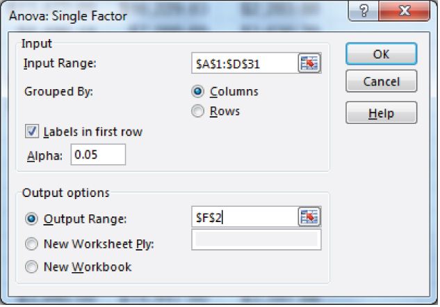
Figure 10.5 ANOVA: Single-Factor dialog box
The Excel ANOVA Output
Figure 10.6 shows the output of the ANOVA: Single-Factor data analysis add-in. As indicated in the output range in Figure 10.5, the analysis output begins in cell F2. Cells F6:F9 show the four hospitals. Cells C6:G9 show the number of observations for each hospital. Cells H6:H9 show the sum of costs for each hospital, and cells I6:I9 show the average cost for each. The variance in cells J6:J9 is calculated by the standard variance formula given in Equation (6.3). An alternative way of calculating the within group variance would be to multiply each of the variance numbers by the degrees of freedom for each hospital (29) and sum them. Doing so would produce the same number as that shown in cell G15 as the within groups sum of squares. Cells G14, G15, and G17 show the between groups, within groups, and total sum of squares, respectively. You may note that these are the same values obtained in Figure 10.3 by our calculations. The mean square values in cells H14 and H15, which represent the sum of squares divided by the appropriate degrees of freedom, are also the same as those calculated in Figure 10.3, as are the F test value and the probability of the F.
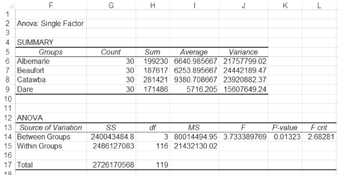
Figure 10.6 Output of the ANOVA: Single-Factor data analysis add-in
The =FINV() Function
The additional information in Figure 10.6 is the number in cell L14 titled F crit, which stands for F critical. F crit is the value that must be reached by the F test (the division of MSB by MSW) in order to be at the 0.95 level of confidence. The value of F crit can be obtained with the =FINV() function. The =FINV() function takes three arguments: the level of significance (in this case, 0.05), and the degrees of freedom in MSB and MSW. The F crit statement that produces the value in cell L14 L13 is =FINV(0.05,3,116).
The F test as discussed thus far provides a way to determine if a numerical variable treated as dependent is actually independent of a categorical variable that takes on more than two values. Why could the same F test not be used if the categorical variable takes on only two values, thus eliminating the need for the t test? The answer is that it could, but the t test has at least one advantage over the F test. The F test is always a two-tail test. There is no equivalent to the one-tail t test for the F test. In consequence, the t test remains useful if the categorical variable in question takes on only two values.
Where Do the Differences Lie in ANOVA?
The interpretation of the F test in either Figure 10.3 or Figure 10.6 is that at least one among the four hospitals under consideration is different from at least one other hospital in average cost. This is not a conclusion about the 30 sample observations from each hospital. Rather, it is a conclusion about all the discharges from the hospitals, assuming that the 30 discharges studied were drawn at random from all discharges. But determining that at least one hospital differs from at least one other is not the most satisfactory outcome. It might be pretty easy to decide that Catawba County hospital has higher costs (an average of $9,380.71 per discharge) than Dare Regional (an average of only $5,716.21). But what do we decide about Beaufort Municipal (at $6,253.90)? Does it have lower costs than Catawba, or higher costs than Dare? These questions cannot be answered directly by ANOVA, but they can be answered by several different statistical tests. Unfortunately for users of Excel, most of these tests rely on something called the studentized range statistic, which is often designated qr. Excel does not provide probability distributions for the studentized range statistic, so this section will discuss a technique provided by Winer ([1962]). This technique can provide a direct comparison between each hospital and every other hospital, and the result can be interpreted using the F distribution, for which Excel does provide exact probabilities.
ANOVA: The Test of Differences
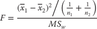
In our discussion of this statistical technique, it will be referred to as the test of differences between two means in ANOVA. It could equally be used to test one mean in comparison with all other means or two means in comparison with two others. However, this discussion will concentrate only on the test of two means at a time. The formula for this test is given in Equation 10.5.
where ![]() is the mean of the first group to be compared,
is the mean of the first group to be compared, ![]() is the mean of the second, and n1 and n2 are the respective sizes of the two samples. MSW is the mean square within groups taken from the original F test.
is the mean of the second, and n1 and n2 are the respective sizes of the two samples. MSW is the mean square within groups taken from the original F test.
Equation 10.5 results in an F test with one degree of freedom in the numerator and degrees of freedom for MSW (the mean square error) in the denominator. We can use this F test to determine which of the four hospitals is different from the others. If we do so, there will be six comparisons, as shown in Figure 10.7, which shows each hospital in cells F22:F25. They have been reordered; the hospital with the lowest average cost is listed first. Cells G22:G25 give the average cost per discharge for each hospital. The hospitals have been listed again in cells H20:K20, with their average costs given in cells H21:K21. Incidentally, the hospitals and their costs in cells H20:K21 were generated by copying cells F22:G25 and using the Paste Special ⇨ Transpose command in cell H20. The six meaningful hospital cost comparisons are given in the cells above and to the right of the main diagonal of the resulting table. These six comparisons contrast each hospital with every other hospital.
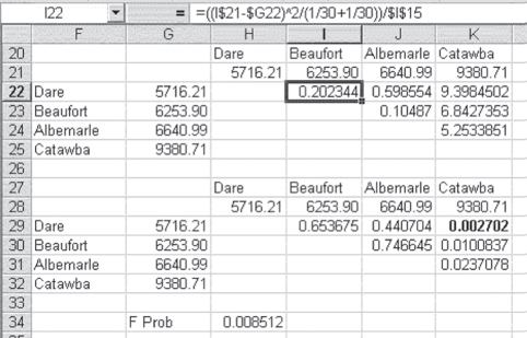
Figure 10.7 Test of differences between two means in ANOVA
The data in Table 10.2 represent the calculation of the formula given in Equation 10.5. The formula bar gives the calculation for cell I22. This is a comparison between Dare Regional and Beaufort Municipal. The dollar sign ($) convention as given in the formula bar allows the formula for cell I22 to be copied to the other five cells to produce the result for each comparison. The fact that the sample size is the same for each hospital makes the term (1/30 + 1/30) appropriate for each comparison. The last term, $I$15, refers to the mean square within groups (MSW), given in cell I15 in Figure 10.6.
Table 10.2 Formulas for Figure 10.7
| Cell or Column | Formula | Action/Note |
| I22 | =((I$21–$G22)^2/(1/3011/30))/$I$15 |
Copied to cells J22, K22, J23, K23, and K24 |
| I29 | =FDIST(I22,1,116) Degrees of freedom in the numerator is 1 because we are comparing 2 events (i.e., n = 2) and DoF = n− 1 degrees of freedom in the denominator is equal to the DoF of MSW, which is 116. |
Copied to cells J29, K29, J30, K30, and K31 |
| H34 | =1–(1–0.05)^(1/6) |
Alpha is chosen to be 0.05 and c = 6 because six tests are being completed. |
The second row in Table 10.2 contains the formula for the probabilities of the F values calculated in Figure 10.7. As you can see from Figure 10.7, the probability of an F as large as the 0.2023 in cell I22 is given as 0.6537 (cell I29). This means that if the average cost for Dare Regional and Beaufort Municipal were actually the same, an F value as large as 0.2023 would be obtained from the formula in Equation 10.5 about 65 percent of the time. Because our alpha level throughout this book is assumed to be 5 percent, we would clearly not reject the null hypothesis that costs per discharge for Dare and Beaufort are the same. But what do we conclude, for example, about Beaufort Municipal and Catawba County hospitals? In this case, the probability of the F value being as large as 6.843 is about 0.01. This number appears to be telling us that the costs per discharge for the Beaufort and Catawba hospitals are different. However, should we reject the null hypothesis that the two hospitals are no different in average costs per discharge? The answer is probably not, which needs a little explanation.
Rejecting/Accepting the Null Hypothesis When Using F Tests
In comparing each of the hospitals with every other hospital, six comparisons are made. And when a large number of comparisons are made following a significant overall F, the overall probability of alpha (α) increases. In other words, we run a higher risk of coming to the wrong conclusion. If we conduct six tests, the overall probability of alpha for all six tests will be 1 – (1 – α)^6. If the initial alpha is 0.05, this produces an overall probability for all six tests of about 0.26. Thus, if we conduct six tests, there is about one chance in four that a difference large enough to reject the null hypothesis at the 0.05 level will occur when we should not reject the null hypothesis. We run the risk of making the Type I error about one-fourth of the time. This risk is really too high.
Protecting against Alpha Inflation: Adjusting the F Probability
To protect against this inflation in the true value of alpha over six tests, we can reduce the actual probability level at which we will reject the null hypothesis by the result of the formula shown in Equation 10.6. In that equation, αAdj is the adjusted value of alpha, and c represents the number of comparisons being made. Taking the cth root of 1 − α would be a daunting task if it were being done with paper and pencil. Happily for us, Excel can take a cth root with very little difficulty. The F probability that provides an overall 0.05 level for alpha for all six tests taken together is given in cell H34 in Figure 10.7. This value is calculated using the Excel formula statement =1−(1−0.05)^(1/6), which is the Excel equivalent of Equation 10.6 when alpha is 0.05 and c is 6. Based on this adjusted alpha for all six tests, we would conclude that only one comparison leads us to reject the null hypothesis of no difference. This is the comparison shown in bold in cell K29 of Figure 10.7—namely, that between Catawba County and Dare Regional. In other words, Catawba's costs are different from those of Dare, but no other average discharge costs are different. With this in mind, the significant F value obtained in both Figures 10.3 and 10.6 is a function of the difference between Catawba and Dare.
It would not always be necessary to make all possible two-group or two-hospital comparisons following a significant overall F. In some cases, it may be sufficient simply to know that there is an overall difference. In turn, the test of differences between hospitals could be ignored. In other cases, it might be decided before the fact that if there are significant overall differences, it is because one group, such as Catawba County hospital, has greater costs than all the other three. In such a case, it would be reasonable to test Catawba against the other three only. This would result in only three comparisons, and the level of αAdj would be, as expressed in Excel, =1−(1−0.05)^(1/3)=0.017.
Assumption of Equal Variances: The Bartlett Test
Like the first t test discussed in Chapter 9, the analysis of variance discussed here assumes equal variance across groups. There are several tests of the homogeneity of variance across groups, but the one discussed here is called the Bartlett test. The Bartlett test is a chi-square test and is carried out with the formula given in Equation 10.7. The formula in Equation 10.7 is somewhat imposing, but, in practice, it is easily calculated using Excel. The result of the calculation is shown in Figure 10.8.
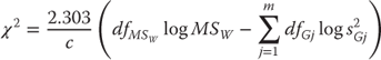
where
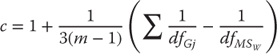
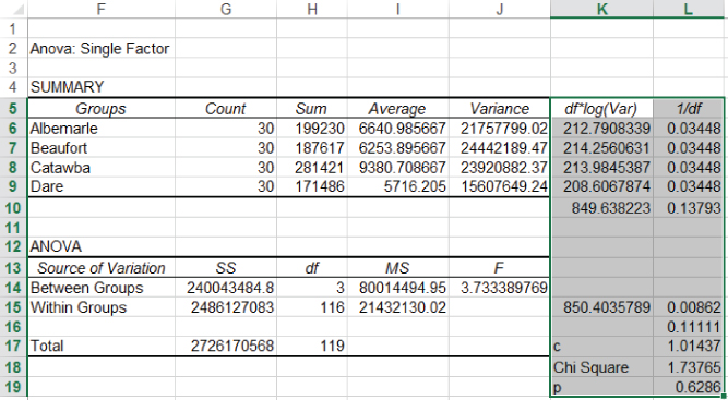
Figure 10.8 Bartlett test for homogeneity of variance: Interpreting the Bartlett test
Figure 10.8 replicates a part of the ANOVA output shown in Figure 10.6. The calculation of the Bartlett test is given in columns K and L. Cells K6:K9 represent the degrees of freedom in each group (cells G6:G9, respectively, minus 1, or 29) times the log of the variance (cells J6:J9). These results are summed in K10, which represents the term in Equation 10.7. Cells L6:L9 are 1 divided by the degrees of freedom in each group, and cell L10 is the sum of these, representing the term in the calculation of the term c. Cell K15 is cell H15 multiplied by the log of cell I15, and cell L15 is 1 divided by cell H15. Cell L16 is the result of the calculation of 1/(3 × (m − 1)), where m is the number of groups being compared. The calculated value of c is shown in cell L17, and the calculated chi-square value is shown in L18. This chi-square statistic has m − 1, or three degrees of freedom. The probability value for a chi-square of 1.738 is given in cell L19 and was found using the =CHIDIST() function. The actual Excel statement is =CHIDIST(1.738,3). Table 10.3 contains the Excel formulas for completing the Bartlett test procedure.
Table 10.3 Formulas for Figure 10.8
| Cell or Column | Formula | Action/Note |
| K6 | =(G6–1)*LOG(J6) |
Copied to cells K7, K8, and K9 |
| K10 | =SUM(K6:K9) |
|
| L6 | =1/G6 |
Copied to cells L7, L8, and L9 |
| L10 | =SUM(L6:L9) |
|
| K15 | =H15*LOG(I15) |
|
| L15 | =1/H15 |
|
| L16 | =1/(3*(4–1)) |
Here the 4 represents m and is the number of groups being compared (i.e., Albemarle, Beaufort, Catawba, and Dare). |
| L17 | =1+L16*(L10–(1/H15)) |
|
| L18 | =(2.303/L17)*(H15*LOG(I15)–K10) |
|
| L19 | =CHIDIST(L18,3) |
Here the 3 represents the degrees of freedom, which is m − 1 again with m being 4. |
The interpretation of the Bartlett test is as follows. If the variances of the four hospitals are, in fact, the same—that is, the null hypothesis is true—we would expect to find a chi-square value as large as 1.738 about 60 percent of the times we drew samples of size 30 from each of the four hospitals. Because the likelihood of finding a chi-square value as large as 1.738 is so high, we will conclude that, in fact, the variances are the same.
The Bartlett test is one way of testing for the homogeneity of variance between the groups compared in ANOVA. However, it is not an essential part of the ANOVA process. When variances differ across the groups in the order of magnitude—for example, of 1 to 3 (i.e., the variance of one group is three times as large as the variance of another)—the results of ANOVA will not be greatly affected. Unless differences across the groups exceed the level of 1 to 3, ANOVA can be used with confidence.
Before we leave the one-way analysis of variance, it is important to comment on sample sizes. In the example given, all four hospitals contributed an equal number of observations—30—to the analysis. In many cases, it is not possible to obtain an equal number of observations for each group. In such a situation, everything that was discussed earlier in regard to ANOVA applies nonetheless. It is simply necessary to ensure that the appropriate number is used for nj and for degrees of freedom for each group.
10.2 ANOVA for Repeated Measures
Two essentially different types of t test were discussed in Chapter 9. The first of these was a t test for differences between two unrelated groups. One-way analysis of variance is the multiple group extension of that t test. The second was the t test for a single group measured two times. The extension of that test is ANOVA for repeated measures. In this case, one group of people, or of organizations, is measured on some variable more than two times. The primary question: Is there is any difference between the several measurements?
Repeated ANOVA tests the equality of means and is used when all components of a random sample are measured under a number of different conditions.
One of the questions that are of concern to the hospital alliance has to do with the cost of readmissions. In particular, it is suspected that the later admissions in a string of readmissions for the same person are likely to be more expensive than the earlier admissions. It is not always easy to track readmissions, particularly if they are at different hospitals. However, one of the hospitals in the alliance has been able to put together a list of several hundred people who were admitted to any one of the hospitals at least three times in the past three years. They have selected a random sample of 12 of these people and have determined the actual cost of each admission. The question then is, do these costs differ from admission to admission? If we were considering only a single readmission, it would be possible to use the t test for related data, comparing the mean for the first admission with the mean for the second. Because we are considering three admissions, it is more appropriate to use analysis of variance for repeated measures. It might also be pointed out that 12 people is a very small sample. Thirty people would be better. But 30 people would make an example that would take up too much spreadsheet space to be easily shown in this book. So we will stick with the smaller sample for illustrative purposes.
Variation within Repeated ANOVA: Effect versus Residual Variation
In considering analysis of variance for repeated measures, the total variation in the data (SST) can be divided into the variation between people—or between groups—(SSB) and the variation within people or groups (SSW). In general, differences that may exist between people or groups (SSB) are not of interest to us. Rather, we are interested in the differences within people or groups (SSW). In the example discussed here, differences within people are differences that may reflect different costs of hospital stays, depending on which admission is being considered. But SSW can also be divided into two sources of variation. One source is the variation that is due to the differences in effect (i.e., costs of first, second, or third admissions) and is referred to as SSA. The other is the variation that cannot be explained by whether the admission is first, second, or third. This last variation is generally referred to as residual variation (SSR).
The formula for the variation within people (or groups) is given in Equation 10.8. Equation 10.8 says that the mean for each person or group i, ![]() , is subtracted from each observation for the person or group. The result is squared and summed over all people. In the example under discussion here, each person was admitted three times to the hospital. The average cost of all three admissions is subtracted from the cost of each and is then squared. And then each of these three values is summed over all 12 people.
, is subtracted from each observation for the person or group. The result is squared and summed over all people. In the example under discussion here, each person was admitted three times to the hospital. The average cost of all three admissions is subtracted from the cost of each and is then squared. And then each of these three values is summed over all 12 people.
where m is the number of different measurements.
Calculating Effect versus Residual Variation
The initial calculation of SSW can be seen in column D in Figure 10.9, which shows an ID number for each person in the sample in column A and the number of the admission in column B. All admissions for the first seven people are shown in the figure. The data in the spreadsheet depicted in the figure actually occupy the first 37 rows of the spreadsheet. Column C is the cost of each admission for each person. Column D is the initial calculation of SSW.
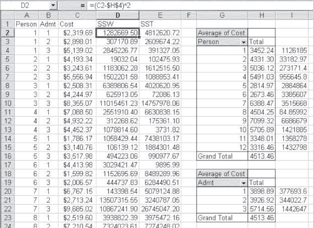
Figure 10.9 Data for ANOVA for repeated measures
The Excel formula used for the calculation is shown in the formula bar in Figure 10.9. This formula indicates that the value in cell H4 was subtracted from the value in cell C2. The value in cell H4 is the mean cost for person 1, which was obtained using the pivot table function and the average option. The dollar sign ($) convention in cell D2 allows that formula to be copied to cells D3 and D4. Unfortunately, the calculation of SSW is a little tedious, requiring that the $H$4 reference be changed to $H$5 for person 2, $H$6 for person 3, and so on. The result of the calculation of SSW is shown in cell L4 in Figure 10.10. As the formula bar in that figure shows, SSW is the sum of cells D2:D37 from Figure 10.9. Table 10.4 contains the formulas for calculating the ANOVA for repeated measures.
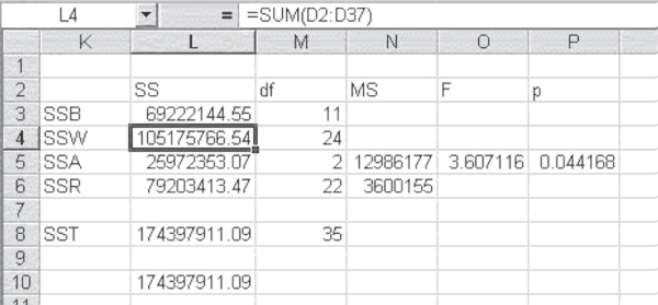
Figure 10.10 Results of ANOVA repeated measures
Table 10.4 Formulas for Figure 10.9
| Cell or Column | Formula | Action/Note |
| D2 | =(C2–$H$4)^2 |
Copied to cells D3 and D4 |
| D5 | =(C2–$H$5)^2 The logic for cells D2 and D5 continues for each group of three subsequent cells through cell D37. |
Copied to cells D6 and D7 NOTE: Increment the row number, X, for the $H$X command for each group of three. |
| E2 | =(C2–$H$16)^2 |
Copied to cells E3:E37 |
| I4 | =(H4–$H$16)^2 |
Copied to cells I5:I15 |
| I20 | =(H4–$H$23)^2 |
Copied to cells I21:I22 |
SSA, which is the variation due to differences in admission costs or effect, is calculated from the formula in Equation 10.9, which indicates that SSA is calculated by subtracting the grand mean from the mean for each admission. In this case, for example, as there are 12 people, there will be 12 first admissions averaged, and then 12 second and 12 third. Because this is a repeated measures ANOVA, n refers to the number of people or groups measured. There are n, or 12, people observed in this case, but mn, or 36, total admissions. The squared value for the m, or three, admissions is then summed and multiplied by the number of people in the study, or 12. The result of this calculation is given in cell L5 in Figure 10.10. Table 10.5 contains the formulas for calculating the ANOVA repeated measures results in Figure 10.10.
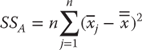
Table 10.5 Formulas for Figure 10.10
| Cell or Column | Formula | Action/Note |
| L3 | =3*(SUM(I4:I15)) |
|
| L4 | =SUM(D2:D37) |
|
| L5 | =12*(SUM(I20:I22)) |
|
| L6 | =L4–L5 |
|
| L8 | =L3–L4 |
|
| M3 | =12–1 |
Where 12 is m |
| M4 | =12*(3–1) |
Here the 12 represents m and the 3 represents n. |
| M5 | =3–1 |
Where 3 is n |
| M6 | =(3–1)*(12–1) |
Where 3 is n and 12 is m |
| M8 | =3*12–1 |
Where 3 is n and 12 is m |
| N5 | =L5/M5 |
|
| N6 | =L6/M6 |
|
| O5 | =N5/N6 |
|
| P5 | =FDIST(O5,M5,M6) |
The residual variation, SSR, is the difference between SSW and SSA. It is shown for this example in cell L6 in Figure 10.10. In cell L6, SSR was actually calculated by SSW − SSA. The formula for SSR is somewhat complicated but is as shown in Equation 10.10. In this case, there are 36 observations, m × n or 12 times 3. According to Equation 10.10, for each observation in the data set, the mean across all three admissions for each person ![]() and the mean across all 12 people for each admission
and the mean across all 12 people for each admission ![]() are each subtracted from the individual observation corresponding to each of these means. The grand mean across all observations is added to this value, and the result is squared. Then this figure is added across all 36 admissions.
are each subtracted from the individual observation corresponding to each of these means. The grand mean across all observations is added to this value, and the result is squared. Then this figure is added across all 36 admissions.
The calculation of SSR using the formula in Equation 10.10 is shown in Figure 10.11. The Excel statement for the term for SSR corresponding to the first admission for the first person is shown in the formula bar for cell F2. The value in cell D2 was taken from cell H4 in Figure 10.9, and the value in cell E2 was taken from cell H20, also from Figure 10.9. The grand mean, which is given in cell F1, was taken from cell H16 in Figure 10.9. As the formula bar shows, the value in cell D2 and the value in cell E2 are each subtracted from the value in cell C2. The grand mean in cell F1 is added to this total, and the result is squared. The sum of column F (excluding the mean in cell F1) is not shown, but it is exactly equal to the value shown for SSR in cell L6 in Figure 10.10.
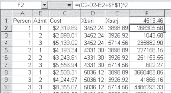
Figure 10.11 Calculation of SSR
Although the between person variance SSB and the total variance SST do not enter into the calculation of the F test, it is useful to know how they are derived. The formula for SST is exactly the same as the formula for SST for one-way ANOVA. That formula is shown in Equation 10.3. In this case, however, nj will be only n because, with repeated measures on the same people or groups, the number of observations for each measurement will always be the same. The formula for SSB is shown in Equation 10.11.
The initial steps in the calculation of both SST and SSB are shown in Figure 10.9. SST is shown in column E and summed in cell L8 in Figure 10.10. The part within the parentheses for SSB is calculated in cells I4:I15 in Figure 10.9, and the sum of those cells is multiplied by measurements (3) in cell L3 in Figure 10.10.
The degrees of freedom in repeated measures of ANOVA are given for this example in column M in Figure 10.10. The degrees of freedom for SSB will always be n − 1. Degrees of freedom for SSW will always be n(m − 1). These, together, add to the degrees of freedom for SST, nm − 1. The degrees of freedom for SSA, m − 1, and the degrees of freedom for SSR, (n − 1)(m − 1), add together to the degrees of freedom for SSW. These respective degrees of freedom are shown in Figure 10.12.
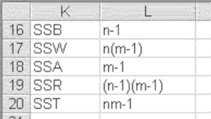
Figure 10.12 Degrees of freedom in repeated measures
The F test for the differences between the costs of admissions is the mean square, due to admissions, MSA, divided by the mean square residual, MSR. These are shown in cells N5 and N6, respectively, in Figure 10.10. The result of the division is shown in cell O5 in Figure 10.10. Cell P5 shows the probability of the F value, 0.044. This value says that if there were no difference in the cost of admissions across the three separate admissions considered, the probability of finding an F value as large as 3.6 would be about four chances out of 100 samples. Because the likelihood is so small under the null hypothesis of no difference, the conclusion is that the cost of admission is not independent of whether the admission is a first time, a first readmission (second admission), or a second readmission (third admission). In other words, the admission timing does matter in determining cost.
Where Do Observed Differences Lie?
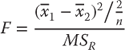
As in one-way ANOVA, it is possible to consider, with the repeated measures design, where the differences between measures (in this case, admissions) might lie. The F test is again a test of the squared difference between two means—in this case, the mean cost of any admission. The formula for the F test is given in Equation 10.12, which is a modification of Equation 10.5. Equation 10.5 recognizes the fact that n is the same for each group and that the error mean square is designated mean square residual (MSR). As with Equation 10.5, ![]() refers to the mean of the first group in the comparison and
refers to the mean of the first group in the comparison and ![]() refers to the mean of the second. This F test has one degree of freedom in the numerator and degrees of freedom equal to that of MSR in the denominator.
refers to the mean of the second. This F test has one degree of freedom in the numerator and degrees of freedom equal to that of MSR in the denominator.
In the case of the cost of the three admissions to the hospital, there could be three comparisons: that between admission 1 and admission 2, that between admission 1 and admission 3, and that between admission 2 and admission 3. The comparison across the three admissions is shown in Figure 10.13. The F test is shown as calculated in cells J29, K29, and K30. The formula for the F test as reproduced in Excel is shown in the formula bar for cell J29. Again, the use of the dollar sign ($) convention, as given in the formula bar, allows the contents of cell J29 to be copied to the other two cells directly. Cells J35, K35, and K36 show the probability of the F value given in the first three cells mentioned. Clearly there is no difference between admission 1 and admission 2, with a p value of 0.971. However, admission 3 appears to be different in cost from both admissions 1 and 2, with p values of 0.028 and 0.030 respectively. But because we have conducted three tests, the adjusted p value in cell H39 gives an overall level of 0.05 for all three tests, based on the formula in Equation 10.6. This says that for an overall level of 0.05 for all three tests, we must have a level of 0.017 for any individual test. This leaves us with the anomalous result that we have found a significant overall F, but with any of the three individual comparisons, we do not find significant F values. Although this is anomalous, it is not uncommon, especially if one is using the stringent criteria of the adjusted alpha level. From a practical standpoint, because there is a significant overall F value, and because the third admission is clearly more costly than the first two, it is appropriate in this case to consider the statistically significant difference to lie with the difference between the first two admissions and the third. Table 10.6 displays the Excel formulas for calculating the F tests in Figure 10.13.
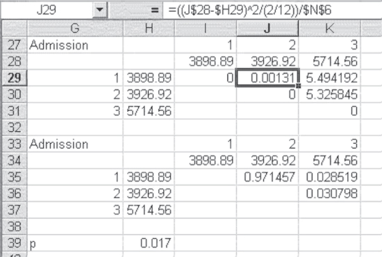
Figure 10.13 Comparison across three admissions
Table 10.6 Formulas for Figure 10.13
| Cell or Column | Formula | Action/Note |
| J29 | =((J$28–$H29)^2/(2/12))/$N$6 |
Copied to cells K29 and K30 |
| J35 | =FDIST(J29,1,22) |
Copied to cells K35 and K36; the degrees of freedom are determined as 1 and 22 because two entities are being compared (i.e., 2 − 1 = 1) in the numerator while the denominator has the same degrees of freedom as the MSR (i.e., (3 − 1)*(12 − 1)). |
Excel Add-In for Analysis of Variance with Repeated Measures
Excel does not provide a specific add-in for analysis of variance with repeated measures when only one group is under consideration (in this case, the one group is the 12 people, each of whom was admitted to the hospital three times). Excel does provide a repeated measures ANOVA when there is more than one group and more than one measure on each group. This is later discussed (in Section 10.3) as what is known as a factorial design.
10.3 Factorial Analysis of Variance
Analysis of variance, like many special topics in statistics, is one to which entire books have been devoted. This chapter considers only one further application of analysis of variance, generally referred to as a factorial design. There are many different types of factorial designs. The one considered here is that in which there is a single numerical variable as the dependent variable and two categorical independent variables. For example, suppose the hospital alliance was interested not only in the differences among the four hospitals of the alliance but also in whether these differences were related to the sex of the patient. To simplify the calculations—and to present some variety in topics—instead of dealing with the cost of admission, this example will deal with the length of stay.
Factorial Example Applied to Hospital Admissions: Length of Stay and Gender
Consider that each hospital in the alliance has divided its admissions for the past year into those for males and those for females. In addition, each hospital randomly selects admissions for 10 males and for 10 females to include in the study. For each of these admissions, the length of stay is recorded and the data are submitted to analysis of variance. Figure 10.14 shows the entire analysis of variance for the data derived from the sample of 10 males and 10 females, taken from each of the four hospitals. Column A shows the name of the hospital. Only the first 22 of 80 admissions are shown in the figure. All entries are males, and 10 are for Albemarle, 10 for Beaufort, and 2 for Catawba. Column B shows the sex of the person admitted. Column C shows the length of stay (LOS). Columns D and E are used in the calculations and are discussed later.
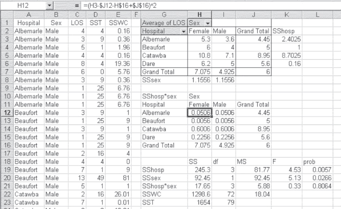
Figure 10.14 ANOVA factorial analysis
Table 10.7 contains the formulas for the calculations in Figure 10.14.
Table 10.7 Formulas for Figure 10.14
| Cell or Column | Formula | Action/Note |
| Create a pivot table for the data with Gender as the columns and Hospital as the rows. | ||
| D2 | =(C2–$J$7)^2 |
Copied from cell D2 to cell D81 |
| E | For Males=(C2–$I$3)^2=(C2–$I$4)^2=(C2–$I$5)^2=(C2–$I$6)^2For Females =(C2–$H$3)^2=(C2–$H$4)^2=(C2–$H$5)^2=(C2–$H$6)^2 |
Copied from cells E2:E11 Copied from cells E12:E21 Copied from cells E22:E31 Copied from cells E32:E41 Copied from cells E42:E51 Copied from cells E52:E61 Copied from cells E62:E71 Copied from cells E72:E81 |
| K3 | =(J3–$J$7)^2 |
Copied from cell K3 to cells K4, K5, and K6 |
| H8 | =(H7–$J$7)^2 |
Copied from cell H8 to I8 |
| J12H16 | =J3=H7 |
Copied from cell J12 to cell J16 Copied from cell H16 to cell I16 |
| H12 | =(H3–$J12–H$16–$J$16)^2 |
Copied from cell H12 to cells H13, H14, H15, I12, I13, I14, and I15 |
| H19 | =20*SUM(K3:K6) |
Where 20 is m*n, and m = 2, n = 10 |
| H20 | =40*SUM(H8:I8) |
Where 40 is q*n, and q = 4, n = 10 |
| H21 | =10*SUM(H12:H15) |
Where 10 is n |
| H22 | =SUM(E2:E81) |
|
| H23 | =SUM(D2:D81) |
|
| I19 | =3 |
Where 3 is q − 1 and q = 4 |
| I20 | =1 |
Where 1 is m − 1 and m = 2 |
| I21 | =3 |
Where 3 is (q − 1)*(m − 1) and q = 4, m = 2 |
| I22 | =72 |
Where 72 is q * m * (n − 1) and q = 4, m = 2, n = 10 |
| I23 | =79 |
Where 79 is q * m * n − 1 and q = 4, m = 2, n = 10 |
| J19 | =H19/I19 |
|
| J20 | =H20/I20 |
|
| J21 | =H21/I21 |
|
| J22 | =H22/I22 |
|
| K19 | =H19/J$22 |
Copied to cells K20 and K21 |
| L19 | =FDIST(K19,I19,I$22) |
Copied to cells L20 and L21 |
The first step in the analysis of variance is to obtain the mean LOS by hospital, by sex, and by sex for hospitals. These values are given in the pivot table, beginning in cell G1. The values in this pivot table were obtained using the average option, as was used in Figure 10.3 and Figure 10.9.
Calculation of SST: Total Sum of Squares Variation
Column D shows the initial calculations for SST, the total sums of squares. SST is one of the least important calculations. However, it is also one of the easiest and is therefore presented first. The formula for total sum of squares is given in Equation 10.13. Although the formula in Equation 10.13 appears complex with its triple summation signs, it is not. The symbols q and m in the formula refer to the number of levels of the first factor and the second factor, respectively. If we consider hospitals as the first factor, then there are four of these, so q = 4. Sex, then, is the second factor, and there are obviously two levels for sex and m = 2. The formula says to begin with the first person for the first hospital and sex group; following the presentation in Figure 10.14, that would be Albemarle and a male. For that person, subtract the grand mean across all hospitals, sex groupings, and people (hence ![]() ), square the result; do this for every person in each sex group across all four hospitals, and sum it all up.
), square the result; do this for every person in each sex group across all four hospitals, and sum it all up.
Column D contains the first part of the calculation. The calculation is the square of the difference between each observation and the grand mean. The Excel formula for the first cell in the column that contains a number (cell D2) is =(C2–$J$7)^2. The dollar sign ($) convention ensures that the grand mean is always used in the subtraction as the formula is copied to each cell in column D. The sum of all 80 calculations in column D is given as SST in cell H23.
Calculation of SSWC: Sum of Squares within Cells Variation
The next sum of squares that may be discussed is SSWC, which is the sum of squares within cells. The sum of squares within cells is that portion of the variation in the data that cannot be attributed either to the admitting hospital or to sex of the patient. Consequently, in this example, SSWC is the error variance. It is calculated using the formula in Equation 10.14, which indicates that a mean value is subtracted from every observation, squared, and summed across all 80 patients. But in this case, the mean value that is subtracted is the mean for each hospital and sex grouping. These mean values are those in cells H3:I6 in Figure 10.14. The initial calculation for SSWC is carried out in column E. The Excel formula for cell E2 is =(C2–$I$3)^2. Cell I3, however, is in the terms given in Equation 10.14 or in this case only the term ![]() . It is the appropriate term to be subtracted only from the first 10 observations (males in Albemarle). For males in Beaufort, the appropriate term changes to cell I4, and so on. This can be a little tedious, but it is necessary for the calculation. The sum of all the calculations in column E is given in cell H22 as 1298.6.
. It is the appropriate term to be subtracted only from the first 10 observations (males in Albemarle). For males in Beaufort, the appropriate term changes to cell I4, and so on. This can be a little tedious, but it is necessary for the calculation. The sum of all the calculations in column E is given in cell H22 as 1298.6.
Calculation of SSrows: Sum of Squares between Rows Variation
The sum of squares due to the differences between hospitals are given in Equation 10.15. The equation is given as SSrows, because hospitals are the rows in the pivot table in Figure 10.14. It should be clear that this is a general formula that applies to any two-factor factorial design, not just to this specific one. The formula for SSrows says that the overall average for all 80 observations is subtracted from the average for each hospital. This average is calculated across all people in a given hospital and both sex groups, hence the designation ![]() . That result is then squared and added across all four hospitals. Because there are m times n, or 20 observations for each hospital, the resulting sum is multiplied by 20. The first step in the calculation of SSrows, or, in this case, SShosp, is given in cells K3:K6. The Excel formula for cell K3 is
. That result is then squared and added across all four hospitals. Because there are m times n, or 20 observations for each hospital, the resulting sum is multiplied by 20. The first step in the calculation of SSrows, or, in this case, SShosp, is given in cells K3:K6. The Excel formula for cell K3 is =(J3–$J$7)^2. The formula in cell K3 can then be copied to the other three cells. The sum of the cells K3:K6 is then multiplied by m times n in cell H19. The Excel formula for H19 is =20*sum(K3:K6).
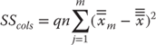
Calculation of SScols: Sum of Squares between Columns Variation
The sum of squares due to differences by sex are calculated in essentially the same way as the sum of squares due to hospitals. Because sex is the column designation in the pivot table in Figure 10.14, the formula for the sum of squares due to sex is given as SScols in Equation 10.16. It can be seen that Equations 10.15 and 10.16 are quite similar. The initial computation of SScols—in this case SSsex—is given in cells H8 and I8 in Figure 10.14. The Excel formula for cell H8 is =(H7–$G$7)^2. The sum of cell H8 and cell I8 is multiplied by q times n (q * n = 40) in cell H20.
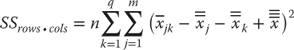
Calculation of SSrows • cols: Sum of Squares Due to Interaction Variation
The only sum of squares left to calculate is what is known as the sum of squares due to interaction. In a factorial design, SSrows and SScols (or the sum of squares due to the hospitals and the sum of squares due to sex) are known as main effects. But there may also be an effect that is due to what is called interaction. The computation of the sum of squares due to interaction is given in Equation 10.17. This equation says to take the mean for each sex and hospital (![]() ), subtract the appropriate mean for sex (
), subtract the appropriate mean for sex (![]() ) and the appropriate mean for hospital (
) and the appropriate mean for hospital (![]() ), add the grand mean (
), add the grand mean (![]() ), square the result, and add it across all sex and hospital groups. The initial calculation of SSrows • cols—in this case, SShosp • sex—is carried out in cells H12:I15. The Excel formula for cell H12, following Equation 10.17, is given in the formula bar in Figure 10.14. The result of the calculations is found in cell H21. It sums cells H12:I15 and multiplies that result by n (which is 3 in this case). As an overall check of the variation calculations, you can confirm that the sum of cells H19:H22 is equal to SST in cell H23.
), square the result, and add it across all sex and hospital groups. The initial calculation of SSrows • cols—in this case, SShosp • sex—is carried out in cells H12:I15. The Excel formula for cell H12, following Equation 10.17, is given in the formula bar in Figure 10.14. The result of the calculations is found in cell H21. It sums cells H12:I15 and multiplies that result by n (which is 3 in this case). As an overall check of the variation calculations, you can confirm that the sum of cells H19:H22 is equal to SST in cell H23.
The degrees of freedom for this analysis are given in cells I19:I23. These degrees of freedom are calculated according to the equations shown in Figure 10.15. It should also be noted that the degrees of freedom shown in cells I19:I22 add to the total degrees of freedom in cell I23.
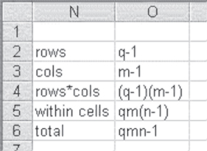
Figure 10.15 Degrees of freedom in two-factor factorial ANOVA
There are three F tests of interest in this analysis. There is an F test for the main effect of hospitals, an F test for the main effect of sex, and an F test for the interaction between the two. The divisor in each of these F tests is the within cell variation SSWC. The mean square values for each of these four elements are given in cells J19:J22, and are the SS values divided by degrees of freedom. The F tests are given in cells K19:K21, and the probabilities of these F values, based on =FDIST(), are given in cells L19:L21. The conclusion from these F tests and their probabilities is that there is a main effect due to hospitals (length of stay is not independent of hospital) and a main effect due to sex (length of stay is not independent of sex), but there is no effect due to interaction.
Excel Add-In for Factorial ANOVA
Excel provides two add-ins in the Data Analysis package for factorial analysis of variance. Only one of those, ANOVA: Two-Factor with Replication, is discussed here. This is the analysis that will produce the results given in Figure 10.14. To carry out the analysis using ANOVA: Two-Factor with Replication, it is necessary first to rearrange the data in Figure 10.14 as they are shown in Figure 10.16. Only the observations for Albemarle and the first five observations for males and females, respectively, are shown for Beaufort in Figure 10.16. The remaining observations continue to row 41 of the spreadsheet. It should be clear that the observations for males are shown in column B and those for females are shown in column C. Also shown in Figure 10.16 is the ANOVA: Two-Factor with Replication dialog box for carrying out the analysis. In that dialog, the input range is given as $A$1:$C$41. This indicates that Excel recognizes that there will be a row of labels at the top of the data and a row of labels in the left column. Rows per sample is given as 10, which means Excel will appropriately treat each 10 rows as a different set of observations. The output range is given as $E$2, which means the output will begin in that cell.
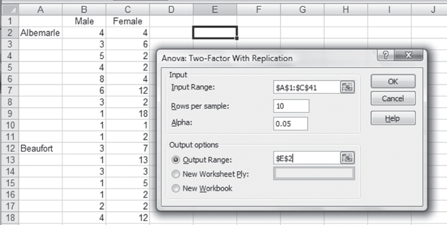
Figure 10.16 Data arrangement for ANOVA: Two-Factor with Replication
ANOVA in Excel Using the Data Analysis Package: Step-by-Step Instructions
Follow these step-by-step instructions to invoke the Data Analysis package in Excel and complete the required inputs for ANOVA output.
- Go to the Data ribbon, in the Analysis group, and click the Data Analysis option.
- After you click the Data Analysis option, a screen resembling Figure 10.16 will appear. In that screen choose the ANOVA: Two-Factor with Replication option. A dialog box, as shown in Figure 10.16, will appear.
- In the Input Range box, enter $A$1:$C$41 or highlight cells A1 through C41.
- In the Rows per sample field, enter 10.
- Click the Output Range radio button, and enter $E$2 in the field.
- Click OK, and the ANOVA output will be created.
Partial results of the ANOVA: Two-Factor with Replication are shown in Figure 10.17. Only the ANOVA table is shown in the figure, but several tables of averages precede the ANOVA results; they occupy rows 2 to 35 but are not shown in the figure. As the figure shows, the results of the Excel ANOVA add-in are the same as those calculated in Figure 10.16. The only difference is the value of Fcrit, given in column K. Again, these are the levels that the F values would have to reach to be significant at the 0.05 level.
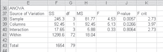
Figure 10.17 Results of ANOVA: Two-Factor with Replication
When one-way analysis of variance was discussed, we indicated that both the formulas and the Excel add-in allowed for different sample sizes across the different groups. Neither the formulas given in this section (for a two-factor ANOVA) nor the Excel add-in permits unequal group sample sizes. It is possible to carry out two- or multifactor analysis of variance with unequal sample sizes in groups. However, the analysis becomes much more complicated and is often more easily performed using dummy variables in multiple regression, which is discussed in Chapter 13.
Repeated Measures in a Factorial Design
The title of the Excel add-in ANOVA: Two-Factor with Replication suggests that at least one of the factors is being measured more than one time. However, using the ANOVA: Two-Factor with Replication add-in for a repeated measure design is not as straightforward as one might wish. As indicated in Figure 10.17, the results are not appropriate to repeated measures on the same set of persons or organizations. The results seen in Figure 10.17 are appropriate, as used in the figure, to a single measure on any included observation.
If the Excel add-in for ANOVA: Two-Factor with Replication is actually used to carry out analysis of variance in a factorial design wherein one variable is measured more than one time, some additional work must be done to get to the appropriate answers. To see that, let us consider a simple example. The data in Figure 10.18 show the length of stay for five men and five women for three different hospital admissions. This represents a factorial design with repeated measures on one variable: hospital admissions. The observation in cell B2, 4, represents a four-day stay for the first man on the spreadsheet. Cell B7 represents the same person's length of stay for his second admission, and cell B12 represents his length of stay for his third admission. Similarly, the 4 in cell C2 represents the length of stay for the first woman on the spreadsheet. Her second stay is represented by cell C7, and her third stay is represented by cell C12. If we use the ANOVA: Two-Factor with Replication add-in to analyze these data, the result is as shown in Figure 10.19. The conclusion that one would draw from this analysis is that there is a difference among the three admissions, but not between the two sexes, in length of stay. This would be based on the fact that the probability for the F related to the samples (the three admissions) is less than 0.05, whereas the probability related to the columns (male and female) is not less than 0.05. We would also conclude no interaction effects.
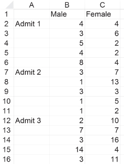
Figure 10.18 Simple data for repeated measures in a factorial design
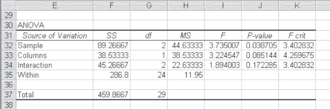
Figure 10.19 ANOVA results for repeated measures in a factorial design
Dividing within Cell Variation in Repeated Measures ANOVA
But this conclusion would not take into account the fact that the three admissions were for the same group of people. In comparing what is given in the ANOVA printout (Figure 10.19) with what is appropriate for a repeated measures design, Figure 10.20 (adapted from Winer [1962]) is useful. As the figure shows, the between cell variation is the same for both repeated and nonrepeated measures. It can be divided into variation due to the columns, variation due to the rows, and the interaction between columns and rows. Where the nonrepeated measure design has only one error term, however—that being the within cell variation—the repeated measures design has two error terms. The within cell variation can be divided into variation due to subjects within groups (one source of error) and variation due to rows (the repeated measure) times subjects within groups (the second source of error). It turns out that the appropriate error term to construct the F test for differences between columns is subjects within groups, whereas the appropriate error term for differences between rows and for the column and row interaction is rows times subjects within groups. Thus, the F test for nonrepeated measures is not appropriate for the repeated measures case.
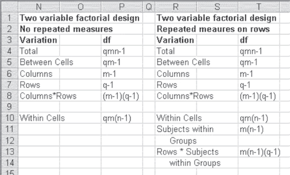
Figure 10.20 Sources of variation and degrees of freedom in factorial designs
Using Excel to Calculate within Cell Variation
To find the values for subjects within groups and for rows times subjects within groups, it is necessary to have the mean value for each person across all measures, something not produced by the Excel add-in. Figure 10.21 shows the analysis for two factors when one is a repeated measure. The average for each person across all measures is obtained in cells E2:F6. As there are 10 people, there are 10 averages. The way in which the average is produced is shown in the formula bar. This can be copied directly to all the cells in E2:F6 to obtain the appropriate average values. Cells E14 and F14 contain the overall average for men and the overall average for women. The formula for the sum of squares for subjects within groups is given in Equation 10.18. This equation says to take the average for each person across all three measures. The designation ![]() means that the ij observations are nested within the k measures. From the average the overall mean is subtracted for each level of j. The result is then squared, summed, and multiplied by the number of repeated measures.
means that the ij observations are nested within the k measures. From the average the overall mean is subtracted for each level of j. The result is then squared, summed, and multiplied by the number of repeated measures.
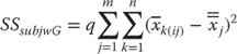
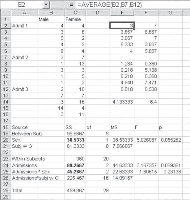
Figure 10.21 Appropriate analysis for repeated measures, two-factor design
The initial steps in this operation can be seen in cells E8:F12. Cells E14 and F14 contain the mean for each sex group (![]() ). The Excel formula for cell E8 is
). The Excel formula for cell E8 is =(E2-E$14)^2. The dollar sign ($) convention allows this formula to be copied to every cell in E8:F12 to produce the terms to be summed for subjects within groups. The formula is completed in cell C21 by multiplying the sum of E8:F12 by 3, the number of repeated measures.
The appropriate analysis of variance table is shown in cells A18:G28. The sources of variation are divided into those that are between subjects and those that are within subjects. The three quantities in bold are those that came from the Excel analysis shown in Figure 10.19. Subjects within groups, plus the column variable—sex—adds to the total between subjects variation of 99.87. Subtracting the between subjects variation from the total variation (cell C28) provides the total for within subjects variation. Subtracting the two values given in Figure 10.19 for admissions and the interaction term produces the term admissions times subjects within groups. The degrees of freedom appropriate to each of these sources of variation are given in column D. The appropriate F test for the difference between the sexes is the mean square for sex divided by the mean square for subjects within groups. The appropriate F test for both admissions and the interaction term requires the mean square for admissions times subjects within groups as the divisor. When these appropriate tests are carried out, we would no longer conclude that there is a difference across admissions, as we incorrectly concluded in Figure 10.19. Table 10.8 contains the formulas for the ANOVA Factorial Analysis in Figure 10.21.
Table 10.8 Formulas for Figure 10.21
| Cell or Column | Formula | Action/Note |
| E2 | =AVERAGE(B2,B7,B12) |
Copied from cells E2:F6 |
| E8 | =(E2–E$14)^2 |
Copied from cells E8:F12 |
| E14 | =AVERAGE(B2:B16) |
Copied from cells E14:F14 |
| C21 | =3*SUM(E8:E12) |
Where 3 is q |
| C20 | =38.53333 |
Given in previous ANOVA, Figure 10.19 |
| C19 | =C20+C21 |
This creates the between subjects source variation. |
| C23 | =C28–C19 |
This creates the total within subjects variation. |
| C26 | =C28–C23 |
This creates the within subjects interaction variation for admissions and subjects within groups. |
| D19 | =9 |
Where 9 is m * n − 1, m = 2, n = 5 |
| D20 | =1 |
Where 1 is m − 1, m = 2 |
| D21 | =8 |
Where 8 is m*(n − 1), m = 2, n = 5 |
| D23 | =20 |
Where 20 is m * n * (q − 1), m = 2, n = 5, q = 3 |
| D24 | =2 |
Where 2 is q − 1, q = 3 |
| D25 | =2 |
Where 2 is (m − 1)*(q − 1), m = 2, q = 3 |
| D26 | =16 |
Where 16 is m*(n − 1)*(q − 1), m = 2, n = 5, q = 3 |
| E20 | =C20/D20 |
Copied to cell E21 |
| E24 | =C24/D24 |
Copied to cells E25 and E26 |
| F20 | =E20/E21 |
Copied to cells F24 and F25 |
| G20 | =FDIST(F20,D20,D21) |
|
| G24 | =FDIST(F24,D24,D$26) |
Copied to cell G25 |
ANOVA and Lean/Six Sigma Practices within the Health Care Industry
It must be noted that ANOVA does not stand alone when applied out in the field. The vast majority of the time it is employed under the auspices of Lean and Six Sigma. Lean and Six Sigma are approaches to improving processes. Manufacturing has applied Lean/Six Sigma to production systems very successfully over the past 30 years in one shape or form (e.g., statistical process control, Toyota Production System, just-in-time inventory). Although health care professionals do not like to think of health care as a production system, health care does have a production system. However, health care workers are not production workers but knowledge workers. In turn, the principles of Lean and Six Sigma can be applied to health care.
The goal of Lean is to reduce waste and cut lead times, while the goal of Six Sigma is to reduce variation and improve quality. ANOVA is employed in the Six Sigma arena to analyze data and ferret out where process variation occurs. Most health care professionals understand hypothesis testing and its use in areas such as medical/drug testing. However, simply put, hypothesis testing and in turn ANOVA are employed to find out “what depends on what.” For example, “Does lab testing lateness depend on day of the week?” By employing ANOVA to analyze changes made to a process (e.g., alter the lab testing schedules), the source of variation can be identified and i process changes can then be implemented that reduce the identified variation. All this leads to the goal of Six Sigma, reduced variation, while pushing to meet the goal of Lean, which is waste reduction and reduced lead times. In all, ANOVA is a very powerful tool within the Lean Six Sigma arena to identify variation and begin the improvement process. It should be noted that entire textbooks and courses are dedicated to Lean Six Sigma. The authors encourage readers to seek out material in these topics as this is only a very brief statement on the area of Lean Six Sigma.