
9.5. Appendix – Alternative Simulation Approaches
These days simulators are everywhere. They are widely used to help 'designers' (architects, urban planners, engineers, military strategists, pharmacologists) understand all sorts of complex things. Simulators as thinking tools include virtual buildings, highway simulators, models of nuclear power stations, water-supply simulators, aircraft flight simulators, virtual battlefields and even virtual hearts. Popular video games like SimCity, Tomb Raider, Formula One, Grand Theft Auto and The Sims all contain simulation engines that control what happens on the screen and animate the vivid and detailed images.
Simulators are of three main types that each use different concepts and building blocks to represent how things change through time. Besides system dynamics, there is also discrete-event simulation and agent-based modelling. Associated with each of these simulation approaches are thriving communities of academics and practitioners and a huge repertoire of models they have developed. There are frequent overlaps in the problem situations to which different simulation approaches are applied. Hence, it is useful for system dynamics modellers (which includes anyone who has reached this point in the book) to be aware that other 'simulationists' exist and to appreciate their worldview.
9.5.1. From Urban Dynamics to SimCity
As a start consider SimCity, a popular yet serious videogame that 'makes you Mayor and City Planner, and dares you to design and build the city of your dreams ... Depending on your choices and design skills, Simulated Citizens (Sims) will move in and build homes, hospitals, churches, stores and factories, or move out in search of a better life elsewhere' (Maxis Software Toys Catalog, 1992, p. 4). The central concept of city attractiveness that lies behind SimCity (even its most recent versions) is reminiscent of Urban Dynamics. A city's attractiveness depends on the quality of its infrastructure and plays a central role in drawing residents (Sims) to the city, or making them leave.[] However, the detailed visual and spatial representation of city infrastructure (with individual icons for commercial and residential buildings, roads, mass transit, police stations, fire departments, airports, seaports and stadiums as shown in Figure 9.32) point to a very different underlying simulation engine whose concepts and equations are far more disaggregated – not unlike an agent-based model. I stop short of saying that SimCity is a true agent-based model or cellular automata as I have never inspected its equations and, as far as I know, they are not accessible to game players. Hence, I use SimCity simply to show that dynamic phenomena can be dressed in a variety of computational clothing.[]
[] It is no accident that, conceptually, SimCity resembles Urban Dynamics. As the game's creator, Will Wright, explains: 'SimCity evolved from Raid on Bungling Bay, where the basic premise was that you flew around and bombed islands. The game included an island generator, and I noticed after a while that I was having more fun building islands than blowing them up. About the same time, I also came across the work of Jay Forrester, one of the first people to ever model a city on a computer for social-sciences purposes. Using his theories, I adapted and expanded the Bungling Bay island generator, and SimCity evolved from there' (quote from Friedman, 1995).
[] I will not pursue agent-based modelling any further here and refer the interested reader to Robertson (2006) for an informative introduction.
Figure 9.32. Screen shot from the original 1989 SimCity showing a spatial representation of city infrastructure
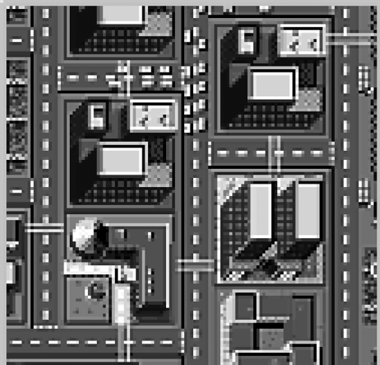
Source: Screen shot from 1989 SimCity by Maxis, © Electronic Arts EA, http://simcity3000unlimited.ea.com/us/guide/
9.5.2. Discrete-event Simulation and System Dynamics
To probe how other simulationists view time-dependent problems I turn to a comparison of discrete-event simulation and system dynamics,[] drawing on work by Morecroft and Robinson 2005.[],[] Figure 9.33 shows a comparison of two models of a natural fishery. Readers are already familiar with the system dynamics model on the right (which was presented in Chapter 1). On the left is an equivalent discrete-event model. Here the fish stock is represented as a queue that is fed by the annual process (cycle of 1 year) of fish replenishment. New fish are sourced from outside the model by the 'source' on the left of the diagram. Initially, there are 200 fish in the sea and the maximum size of the fishery is assumed to be 4000 fish, which are the same numerical values used in the system dynamics model. Fish regeneration is represented as a linear, but random, function of the number of fish in the sea. Fish grow at an average rate of 20 per cent per year, varying according to a normal distribution with a standard deviation of 2 per cent. The limit to growth of 4 000 is represented as a discrete cut-off, which does not allow the fish population to exceed this limit.
[] Discrete-event simulation is a big subject in its own right and readers can find out more from Pidd (2004), Robinson (2004, 2005).
[] These two models were developed independently by the authors (one an expert in system dynamics and the other an expert in discrete-event simulation), based on facts and data in the briefing materials for Fish Banks, Ltd (Meadows et al., 2001). Each of us adopted the normal model conceptualisation and formulation conventions of our respective fields so the resulting models would be a valid comparison of the two approaches.
[] My thanks to Stewart Robinson for permission to include in this appendix the discrete-event models and simulations that come from his part of our joint project.
Figure 9.33. Comparison of discrete-event and system dynamics models of a natural fishery
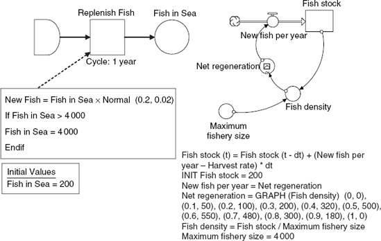
There are some clear differences in the two representations. The system dynamics model uses stocks and flows while the discrete-event model uses queues and processes. Nevertheless, despite the new symbols, there is a clear equivalence between stocks and queues on the one hand, and between flows and processes on the other. Significantly, the feedback structure is visually explicit in the system dynamics model but hidden within the equations of the discrete-event representation. The discrete-event model deliberately includes randomness in the regeneration of fish as this is seen as a process that is subject to variability, but which is not present in the system dynamics version. Meanwhile, the relationship between fish stocks and fish regeneration is non-linear in the system dynamics model, but linear in the discrete-event model.[]
[] For such tiny models as these it is possible in principle to make the formulations identical, but that would contradict the intended independence in the work of the two modellers as outlined in footnote 10.
Time charts from the discrete-event simulation model are shown in Figure 9.34. This chart is the output from a single replication (a run driven with a specific stream of random numbers). If the random number seeds were changed to perform further replications, the exact pattern of growth and fish regeneration would alter. Figure 9.34 shows S-shaped growth similar to the pattern from the system dynamics model, but with two distinct differences. First, the growth is not as smooth due to the randomness within the regeneration process. This extra variability is clear to see in the trajectory of new fish. Second, the system dynamics time chart shows an asymptotic growth towards the limit of 4 000 fish, while the discrete-event model hits the limit sharply. Both of these differences in simulated behaviour are of course a result of the model formulations which in turn reflect more fundamental differences in the approach to conceptualising a fishery. For simple models of a natural fishery, the trajectories look quite similar. But the differences become greater as we move to a harvested fishery where the interactions are more complex.
Figure 9.34. Dynamics of a natural fishery from a discrete-event simulation model
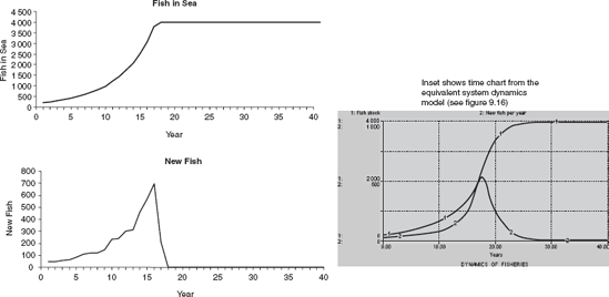
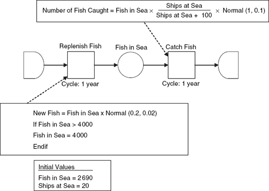
Figure 9.35 shows a discrete-event model of a harvested fishery, which should be compared with the system dynamics model in Figure 9.17. The left side of the process flow diagram is the same as for the natural fishery in Figure 9.33. However, a second process 'Catch Fish' is now added, which represents the catching of fish that are then sent to the sink on the right side of the diagram. The formula for the number of fish caught consists of two parts. The first sees the catch as an increasing proportion of the fish in the sea, a proportion that increases with the number of ships. The formula is non-linear, giving a reduced catch per ship with increasing numbers of ships. It is envisaged that as more ships are fishing in the same area their productivity will fall. The second part of the formula (Normal 1, 0.1) is the modelling of randomness.
Figure 9.35. Discrete-event model of a harvested fishery
The modelling differences identified for the natural fishery apply equally to this case of a harvested fishery: the method of representation, the explicitness of the feedback structure and the inclusion of randomness. Interestingly, the discrete-event model represents the number of fish caught as a non-linear and stochastic function of the number of ships, while the system dynamics model represents this effect as a deterministic linear relation. Further, there is an implied feedback structure in the discrete-event model where the catch is related to the number of fish. A similar feedback is to be found explicitly in the system dynamics model with endogenous investment shown in Figure 9.21. Perhaps the most important distinguishing feature of the discrete-event model, however, is that it now contains two interacting random processes (one in the regeneration of fish and the other in the catch). Discrete-event modellers are well aware that puzzling and counterintuitive dynamics arise when two or more random processes are linked (Robinson, 2004, Chapter 1). These stochastic dynamics are rarely investigated by system dynamics modellers whose interest is feedback dynamics.[]
[] System dynamics models are not entirely devoid of random processes. For example, it is common in factory and supply-chain models to add randomness to demand in order to invoke cyclical dynamics, as demonstrated in Chapter 5's factory model. But system dynamicists do not normally set out to explore surprising bottlenecks and queues (stock accumulations) that stem from interlocking streams of random events.
Figure 9.36. Dynamics of a harvested fishery from a discrete-event simulation model
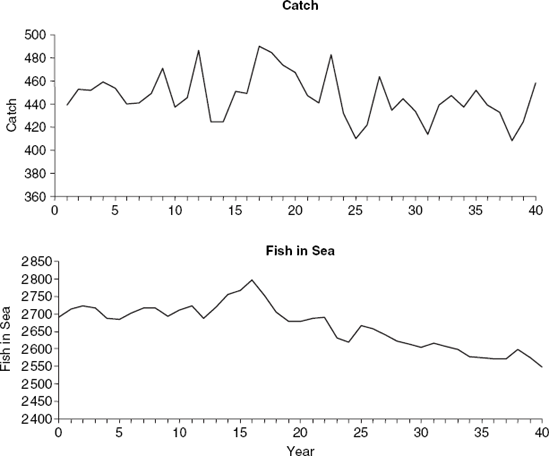
Figure 9.36 shows the results from a simulation of the discrete-event harvested fishery, now with randomness included for the catch and regeneration of fish. As there is 'complex' randomness in the model, the simulation has been replicated 10 times, using different random number streams, the results showing the mean of the replications. The use of multiple replications is standard practice in discrete-event simulation modelling for determining the range of outcomes and the mean performance of a system (Law & Kelton, 2000; Robinson, 2004). The time charts show the catch and the number of fish in the sea over a 40 year period. Notice the variation in the annual catch with the mean shifting between just above 400 to just below 500. Similarly, there is some variation in the fish stock, peaking at about 2 800 and falling to about 2 600. Such variation is not surprising given the randomness in the model. It would be difficult to predict the interconnected effect of variations in fish regeneration and fish catch without a simulation.[]
[] Close inspection of the graph for fish in the sea reveals a downward trend, a trend which is confirmed by longer simulations. The phenomenon is explained in Morecroft and Robinson (2005).
The discrete-event model of a harvested fishery was initialised to yield a perfect equilibrium if the two random processes were to be quelled at the start of the simulation. This special condition was achieved by setting the initial number of fish at 2690 which yields an inflow of new fish per year that exactly balances the annual catch of 20 ships. The observed variations in fish stock therefore stem entirely from interlocking streams of random events. There is no direct analogy to Figure 9.36 for the equivalent system dynamics model of a harvested fishery, because when the fleet size is fixed then any simulation that begins in equilibrium (so the inflow of new fish is exactly equal to the catch) remains in equilibrium. The time charts are flat lines that say nothing about fishery dynamics. Not so in a discrete-event world, where seemingly equilibrium conditions can yield puzzling variations in performance. The catch can rise and fall significantly for stochastic reasons.
A very different kind of equilibrium test, that examines multiple equilibria and tipping points, applies to the system dynamics model of a harvested fishery. We have already seen an example of such a test in Figure 9.18, which shows a simulation of stepwise changes in fleet size. Here we learn something surprising about the properties of a non-linear dynamical system. There are multiple equilibria of fish stock and ships at sea in which the equilibrium catch is progressively higher as more ships are added to the fishery. Then, at a critical fleet size of around 30 ships, the fish stock and the catch begin to collapse. Thereafter, a reduction to 20 ships or even 10 does not halt the collapse.
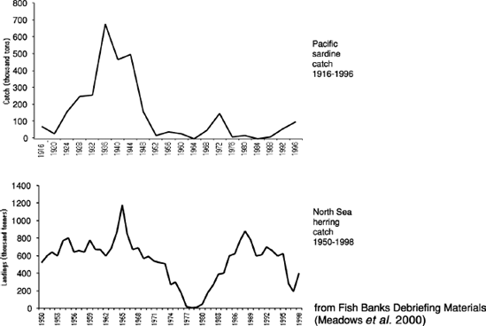
Stochastic variability and tipping points in the catch are two different dynamical phenomena. Yet they are both compatible with real-world data from fisheries. If we look once more at the time series for the Pacific sardine catch and the North Sea herring catch, we see in Figure 9.37 evidence that could support either type of model. The Pacific sardine catch looks like tipping-point dynamics, while the North Sea herring catch looks like extreme stochastic variability.[]
[] The visual fit between time series and simulations is more compelling when each model includes endogenous investment in ships, as in Figure 9.22. There is not the space here to present the equivalent discrete-event model but details can be found in Morecroft and Robinson (2005).
Figure 9.37. Puzzling dynamics of fisheries
9.5.3. Conclusions on Alternative Approaches to Simulation Modelling
What does this fisheries comparison say more generally about alternative simulation methodologies and discrete-event simulation in particular? First it shows there are alternatives approaches that can each provide insight into puzzling dynamics. This is not news, but is useful to include in a book that otherwise concentrates on system dynamics. The comparison also lifts the curtain, at least a few centimetres, on the world of discrete-event simulation. There are important differences not only in technique (queues and activities versus stocks and flows, discrete versus continuous time, stochastic versus deterministic) but also in worldview. System dynamics deals with 'deterministic complexity'. Puzzling dynamic behaviour is explained by feedback structure, which implies that the unfolding future is partly and significantly pre-determined. Within this worldview, problematic situations are investigated by first identifying feedback loops (and their underlying stock accumulations, policies and information flows) and then re-designing policies to change this feedback structure in order to improve performance. Discrete-event simulation deals with 'stochastic complexity'. Puzzling dynamic behaviour arises from multiple interacting random processes, which implies that the unfolding future is partly and significantly a matter of chance. Within this worldview problematic situations are investigated by first identifying interlocking random processes (and their underlying probability distributions, queues and activities) and then finding ways to change or better manage this 'stochastic structure' to improve performance.
A corollary of these differences is that discrete-event simulation is well suited to handling operational detail. Stochastic processes are a concise and elegant way to portray detail within operations. A factory can be conceived as a collection of interacting stochastic machines that process a flow of products. A hospital can be conceived as a collection of stochastic medical procedures that process a flow of patients. Moreover, because of the way random processes release a stream of individual entities (just like individual fans entering a football stadium) then factory models can readily depict detail movement and queues of individual products, and hospital models can track the movement and waiting times of individual patients. This ability to handle detail was not exploited in the fisheries models, but detail is a vital characteristic of most discrete-event models that carries through to their visual interactive interfaces. The resulting look-and-feel of such entity-driven models is much different than system dynamics models with their aggregate stock accumulations and coordinating network of feedback loops. A system dynamics factory model (as in Chapter 5) portrays inventory, workforce and pressure-driven policies for inventory control and hiring – a distant view of operations. In contrast a discrete-event factory model shows machines, conveyor belts, storage areas and shipping bays and if-then-else decision rules that determine the movement of product and usage of machines, all because it tends to focus on a close-up view of operations. But precisely because of its distance from operations, a system dynamics model clearly depicts feedback loops that weave between functions and departments. In contrast a discrete-event model hides such connections or does not attempt to include them at all because it focuses on just one or two functions/departments. The characteristic scope, scale and detail of factors included in a model therefore arise naturally from the modellers' chosen worldview.
Clans are territorial. Their models look so different, and hence it is not surprising that proponents of system dynamics and discrete-event simulation rarely talk. However, communication will improve as understanding grows, and may even spark joint projects. There is also an opportunity for better three-way communication between agent-based modelling, discrete-event simulation and system dynamics.[]
[] Lomi and Larsen 2001 have edited an informative collection of academic papers that illustrate the wide range of ways in which simulation methods have been applied to understanding dynamic phenomena in organisations.