
The essence of systems engineering is the need to compose and understand specifications from multiple engineering domains. Because different engineering activities use different modeling vocabularies, any language purporting to be a system-level modeling language must support heterogeneous specification. More specifically, a system-level modeling language must support and integrate multiple modeling paradigms, models of computation, and communication models.
Rosetta’s support for heterogeneous specification is embodied in domains and interactions. Domains provide a basic modeling vocabulary for a facet and define its type. They allow the designer to choose or define a vocabulary for specification that embodies an appropriate modeling paradigm for that specification. Domains enable Rosetta users to write specifications using different modeling paradigms in the same language system. Interactions describe how heterogeneous specifications interact when combined. Defined over domains, interactions move information from one modeling paradigm to another and are further described in Chapter 15.
We have already seen domains at work in facet definitions, where they are used as common vocabulary for defining specifications. Syntactically, each facet’s domain is specified using a type annotation following the facet signature. Packages, components, and other domains use the same definition technique. Semantically, each facet extends its domain by including all definitions from the domain and adding definitions local to the facet. How this extension is realized during elaboration is specified as a part of the domain.
The primary focus of domain definition is providing a specification vocabulary. Where facets describe specific system models, domains define reusable, common constructs for defining new models. Although domains are like facets in many ways, they are not used as components and cannot be instantiated in structural specifications. They serve as definitional building blocks for facets and group collections of similar facets into types.
Domains accomplish their task by defining units of semantics, models of computation, and engineering domain knowledge to varying degrees. Units of semantics declare the basic modeling primitives shared by classes of specifications. State-based specifications all reference the current state and the next state function, regardless of their specific properties. Similarly, signal-based specifications all reference signals and processes. Models of computation constrain units of semantics by providing increasingly concrete definitions for them. Finite state specifications constrain the state type to be finite and discrete, but do not define new state vocabulary. Similarly, infinite state specifications constrain the state type to be infinite and say nothing of discreteness. Finally, engineering domains gather information specific to a particular domain, such as digital design, hydraulics, analog design, or power modeling.
Rosetta supports incrementally defining units of semantics, models of computation, and engineering domain information through extension of basic models. Starting with units of semantics, models of computation are defined and extended. Using models of computation, basic engineering domains are defined and extended to sub-domains. As we shall see in Chapter 15, sharing units of semantics and models of computation provides explicit support for specification composition, abstraction, and refinement.
The first objective of any domain specification is to provide units of semantics declarations. The units of semantics comprise a basic collection of items that represent quantities shared among specifications in a domain. These items take the form of variable, constant, and type definitions. For example, the concepts of state, time, and state change are critical to all state-based specifications. Although these quantities have different properties based on the specifics of a state-based domain, they are always present. Thus, the state_based domain that serves as a basis for all state-based specifications defines these as basic units of semantics. Domains defined from the state_based domain provide different semantics for these items to define different flavors of state_based specifications.
One of the most critical units of semantics definitions specifies the point-of-reference for observation. Examples of such items include state and time as well as position and order. We say that items like state specify the point-of-reference because all observations are performed with respect to them. For example, we specify the values of variables with respect to state in sequential systems or with respect to time in analog systems. Such domain items are not restricted to specifying to time. They may specify spatial position for representing measured values on a surface or events for representing values associated with occurrences.
When a domain provides nothing other than declarations and is defined directly from the static domain, it is informally referred to as a unit-of-semantics domain. Most Rosetta users will never define a new unit-of-semantics domain, but will instead extend existing domains to provide new models of computation or engineering domains. The unit-of-semantics domains must be added with great care. As we shall see in Chapter 15, carefully choosing common items among specifications can profoundly influence the utility of a system specification.
Among the most important aspects of domain definition is providing models of computation. The difficulty in heterogeneous specification is not understanding how values are calculated, but rather how values change over time. When interfacing an analog component with a digital component, difficulties arise when dealing with behaviors of interface items. Specifically, how does the analog view of an input or output map to the digital view it may be interfaced with? The difficulty is not understanding the values that items take, but rather understanding how those values change over time with respect to each other.
As an example, consider the definition of the time quantity in the state_based and continuous_time domains. In the continuous_time domain, the time type is most easily represented as a real number, and the current time as an element of that type:
   state_type :: type is real;
   s :: state_type;
In contrast, in the abstract state_based domain, the state type is left largely unspecified. We know that it is defined, but not what its characteristics are:
   state_type :: type;
   s :: state_type;
The distinction between state in continuous_time and state_based is only that state is constrained to be real. Thus, continuous_time can be defined by extending state_based to include this constraint.
Defining models of computation and communication in Rosetta is accomplished in domains by defining a point of reference and how that point of reference changes. We have seen how time types, values, and functions can be specified. The key is choosing types appropriately and defining operations over those values. The essence of model-of-computation definition is how and when items change value.
Rosetta provides a collection of built-in factions to assist developers in defining models of computation. The most important are the infix operator @ and the next function, present in all domains except static. Literally interpreted, the expression x@s means “the value of x with respect to s.” Thus, @ is a mapping from an item name and a point of reference to a value, and serves as a dereferencing function. Defining the type of s says much about the model-of-computation. If s is real, then we are modeling a continuous system. In contrast, if s is natural, we are modeling a discrete system. More exotic points of references include surfaces and events. If s is a Cartesian coordinate, we are modeling values along a two-dimensional surface. Using this approach, Rosetta models for heat dissipation in semiconductors can be defined. If s is an event, we can model processes and traces in a manner similar to a constraint satisfaction problem (CSP) or the pi-calculus.
By sequencing states and examining their associated environments, the concept of execution or computation is defined. Rosetta provides the next function over the state type to define this sequencing: next maps a state to its next state and can be constrained by referencing any aspect of the facet state. Thus, if x@s defines the value of x in state s, then x@next(s) defines the value of x in the state (or states) following s. Rosetta defines a standard shorthand x’ that is interpreted as x@next(s), or “x in the next state.” Defining next appropriately supports defining various models of computation using the same common syntax. The catch is that one must understand the current domain to understand how state changes.
The properties of next, together with the state type, define how states are sequenced, providing a basis for a model of computation. For example, given an arbitrary state type, the constraint next(s)>s forces the next state to always be greater than the current state. This ensures that the state will always move forward and forces the state type to be infinite. In contrast, if the constraint is removed and the constraint #state in natural is added, the state space becomes finite and states can be revisited. From a quite simple starting point, sophisticated models of computation can be provided.
When a domain provides no new declarations, but adds constraints to units of semantics, it is informally referred to as a model-of-computation domain. Typically, model-of-computation domains are defined by extending a unit-of-semantics domain or another model-of-computation domain. Where unit-of-semantics domains provide a basic vocabulary, model-of-computation domains constrain that vocabulary to define specific mechanism for computing and sequencing values.
As any engineer knows, simply understanding mathematics is not sufficient for solving real-world engineering problems. Mathematics is a prerequisite, but the real work is done using domain-specific knowledge built from that mathematics. When using Kirchoff’s Laws, an electrical engineer rarely thinks of the continuous time model used by those laws. The civil engineer does not think about the dynamics equations underlying bridge design. An engineer works with domain information that abstracts away the need to go all the way back to mathematics. Because these abstractions are based on sound mathematical principles, they are safely used in design.
Engineering design languages must provide this abstract, domain-specific layer or they are not useful. Languages such as VHDL and Verilog specifically address the needs of digital circuit designers. Matlab and Mathematica provide a basis for defining systems that includes collections of libraries for specific engineering domains such as control and signal processing. The UML software specification language provides a basic modeling paradigm with the ability to define profiles for specializing to various software modeling domains.
For example, in digital design the concept of a clock is fundamental to system design. The definitions of event, quiet, rising-edge, and falling-edge are common when observing a clock and should be defined in any domain used for digital system specification. Concrete functions are provided having the following form:
  event(x::bit)::boolean where event(x') == x/=x'
  quiet(x::bit)::boolean where quiet(x') == x=x'
  rising(x::bit)::boolean is event(x) and x=1;
  falling(x::bit)::boolean is event(x) and x=0;
These definitions differ from those provided by unit-of-semantics and model-of-computation domains. First, they reference units of semantics, but unlike model-of-computation domains they do not constrain them. The use of ticked names implicitly references state, but the reference is only to examine values in that state. Second, they declare, but unlike unit-of-semantics domains, they immediately define new functions and variables. Of course, these characteristics are heuristic — it is quite possible to define a new unit-of-semantics in an engineering domain. However, by avoiding this, specifications are easier to write and use.
When a domain adds to a model-of-computation domain new definitions that reference, but do not constrain, units of semantics, it is informally referred to as an engineering domain. Engineering domains are the workhorse of Rosetta specifications. Most specifications written by designers use an engineering domain to define a specific model for a system or component. Unlike unit-of-semantics and model-of-computation domains, engineering domains are easily written and are commonly added to the domain set. Any time Rosetta is used in a new engineering discipline, new component collections are required, or new abstractions are needed for operations on models, engineering domains are the best modeling approach.
Figure 12.1 shows the domain semi-lattice populated with a classical domain set. The null, static, and descendants of the state_based domain are the most heavily used domains and serve as examples in this section. The static and null domains are the only two domains defined as required elements in the base Rosetta system. Users may add new domains or completely replace the domain lattice if necessary for their specification activities.
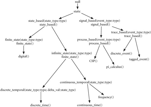
Figure 12.1. Base definition domains in the domain semi-lattice. Two domain signatures in the same node indicate different parameterizations of the same domain.
The null domain refers to the empty domain containing no computation model and no vocabulary. Using the null domain results in a system with only the base Rosetta semantics. It is included to provide a basis for defining domains that inherit nothing from other domains and should only be used by designers who want to start from scratch. The static domain that provides basic mathematics will use null as its type. Unless you intend to define a complete Rosetta domain semantics from scratch, there is little need to reference the null domain. There is no mechanism for constructing null from other domain definitions.
The static domain provides a basic collection of types and functions in a computational model that has no built-in concept of state or time (Figure 12.2). The static domain is defined by using the prelude and unicode packages providing access to basic Rosetta definitions. The original names for the static domain were logic and math, reflecting the domain’s intent of providing basic mathematical definitions. All predefined domains inherit from static and thus share the same mathematical basis. Symbols used to define computational models, @, next, and the state type are not visible in the static domain and cannot be used. Because static has no built-in state or time definitions, domains that inherit from it are free to define their own computational models.
Example 12.2. Skeletal specification of the static domain.
use rosetta.lang.prelude;
use rosetta.lang.unicode;
domain static()::null is
begin
end domain static;
The static domain is most frequently used when defining utility packages where model-of-computation is immaterial or harmful. Operations such as square root and function application, and data types such as integers and sequences, are the same regardless of computation model. The static domain provides common definitions used by all domains and thus all facets. The static domain is also used when defining structural definitions or performance requirements where models of computation are not used. The most important use of the static domain is as a basis for defining remaining domains. Because all domains share the static domain, all domains share the same mathematical structures and Rosetta support functions.
Example 12.1. Power Constraint Specifying a Static Power Limit
The powerLimit facet specifies a limit on the value of an observed item, power. It simply states that the value of that parameter cannot exceed the statically defined value limit. Such a facet would be used as a constraint in a system where power is being consumed and should be limited. The static domain is used because the limit does not change.
  facet powerLimit(power::real; limit:: design real) ::static  is
  begin
    c: power =< limit;
  end facet powerLimit;
When used in a system specification, the domain semi-lattice is typically used to transform the static powerLimit facet to a domain appropriate for composition, with a specification changing power values. The constant nature of the power limit is transformed into a constant limit using the target domain’s computation model. By using the static domain, this specification can be moved virtually anywhere in the domain semi-lattice without sacrificing utility. However, the author of the power facet need not know anything about the target specification. This idea is fully explored in Chapter 15.
Example 12.2. Facet Containing Common Function Definitions and the Equivalent package Specification
The addFns specification defines a pair of utility functions for defining addition operations in digital systems. The static domain is used because there is no concept of time when defining this type of pure mathematical function.
  facet addFns() ::static  is
    export all;
     bitSum(x,y,cin::bit) ::bit is x xor y xor cin;
     bitCarry(x,y,cin::bit) ::bit  is
        (x and y) or (x and cin) or (y and cin);
begin
end facet digital;
This facet can be included in other facets and functions referenced using the dot notation. However, such utility specifications are so common in Rosetta that the package structure is included to define them. As a rule-of-thumb, whenever a facet is defined that includes declarations with no terms, a package should be used instead. Following is the equivalent definition using a package:
  package addFns()::static  is
    bitSum(x,y,cin::bit) ::bit is x xor y xor cin;
    bitCarry(x,y,cin::bit) ::bit  is
        (x and y) or (x and cin) or (y and cin);
  end package addFns;
The state_based domain is a unit-of-semantics domain used to define systems that change state. The state_based domain extends the mathematical capabilities provided by the static domain to include the concept of state and change as traditionally defined. In the static domain, values associated with items cannot change because there is no concept of state. The state_based domain provides the most basic concept of change by introducing the next function and the state type described previously. Specifically, the state_based domain provides the basis for modeling the concepts of state and change by defining (i) an abstract state type, (ii) the current state, (iii) a next state function that derives the next state from the current state; (iv) and an event predicate that is true when an items Value changes from its Value in the previous state. Computations are defined by specifying preconditions on the current state and a relationship between the current and next states that defines computation (Figure 12.3).
Example 12.3. Partial specification of the parameterized and unparameterized state_based domains, showing the declaration of the state type, the current state, and the next state functions.
  domain state_based()::null    is  domain state_based(state_type ::type)::null  is
    state ::type;                    state :: type is state_type;
    s::state;                        s::state;
    next(s::state)::state;           next(s::state)::state;
    event(X::top)::boolean;          event(X::top)::boolean;
begin                            begin
end domain state_based;          end domain state_based;
As a simple example, consider the following definition of a component that sorts its input:
  facet sort(i::input sequence(integer);
           o::output sequence(integer))::state_based  is
    sorted(i::sequence(integer))::boolean  is
      forall(x::0,..((#i)-1) | i(x) =< i(x+1));
  begin
    pre:  true
    post: sorted(o') and -o'=~i
  end facet counter;
This facet defines requirements for a component that sorts its input without specifying a specific sorting algorithm. The state_based domain is used because we must define the output in the next state, but we do not know what the actual state is. Requirements defined by this component can easily be met by either a software or hardware component.
post: sorted(o') and ~o'=~i
The post term defines a post-condition for the component by defining properties on values in the next state. Specifically, o’ refers to the value of o in the next state; post asserts that o’ must be sorted and must be a permutation of the current input, i.
It is exceptionally important to recognize that the following term, similar to a C-like programming statement, is not correct:
next_s: o = sortFn(i);
Terms simply state things that are true. They are not executed and there is no notion of assignment. Although legal in C, where “=” is an assignment operator, in Rosetta this statement asserts that o=sortFn(i) is true. Looking at “=” as equality rather than assignment makes this statement inconsistent because we are asserting that the output is sorted in the same state in which we observe the input. This simply cannot hold. A good rule-of-thumb is to use the tick notation whenever the semantics of assignment is desired.
The key to using state_based domains is recognizing that an un-ticked label indicates the current state and that a ticked label indicates the next state. The state_based tick notation is defined based on the more fundamental state_based domain definitions of current state and the next state function. In reality, the notation x’ is shorthand for the notation x@next(s), where (i) @ refers to the value of a label in a state, (ii) next defines the state following a given state, and (iii) s is the current state. Specifically:
The previously defined sort specification is equivalent to the following expansion:
  facet sort(i::input sequence(integer);
              o::output sequence(integer))::state_based  is
     sorted(i::sequence(integer))::boolean  is
       forall(x::0,..((#i)-1) | i(x) =< i(x+1));
  begin
    pre:  true
    post: sorted(o@next(s)) and ~(o@next(s))=~(i@s)
  end facet counter;
Here the tick notation is replaced by its definition using the next function, and undecorated variables are referenced in the current state. In the state_based domain, the dominant specification methodology is axiomatic specification. Thus, the primary use of @ is to refer to variables in the next state.
Statements of the form R(x,y@next(s)) or xoy@next(s) are used to constrain the value of y in the next state, based on the value of x in the current state. This defines requirements for a computation without defining implementation method. When using the state_based domain, defining a relationship between the items in the current and next state should always be the specification goal. Revisiting the sort specification, the term labeled post defines the relationship between current and next state by defining a relationship between variables in those states. One of the advantages of the the state_based domain and Rosetta generally is that the next state need not be completely defined. If only partial requirements are available or desired, it is necessary only to specify what is known. At high levels of abstraction, such capabilities help the designer avoid over-specification during design exploration.
The state_based domain provides a special function, event, that compares the value of an item in the current and next states to determine if it has changed values. Specifically, event(clk) is true when clk changes values between the current and previous states. The event function supports definition of reactive systems that are triggered by changes in their inputs. A specific example of the event function in action is the definition of a rising clock edge:
rising(clk::bit)::boolean is event(clk) and clk=1;
In this definition, rising is true if event indicates a change in the value of clk and the resulting of the change is a value of 1.
What is happening in the state_based domain is that the model-of-computation is being exposed in the specification. Languages such as C, VHDL, and Lisp have a built in computational model that pervades all definitions. In Rosetta, the model is exposed, allowing integration of specifications in different domains. The price paid for this freedom is the need to think about the model-of-computation in the specification process. Rosetta tries to abstract away as much detail as possible, but some will always remain.
To summarize, the state_based domain should be used whenever a system-level description of component or system is needed. At early design stages, when working at high levels of abstraction, the state_based domain provides a mechanism for describing state transformations without unnecessary details. The state-based domain should not be used when details such as timing are involved in the specification. Furthermore, the state_based domain provides no automatic mechanism for composing component states when developing structural models.
Example 12.3. Register Specification Using the state_based Domain
In the Introduction we explored the definition of a register using the discrete_time domain, examining specification composition and the use of heterogeneous domains. Here we examine a more robust specification in the state_based domain that uses a universally quantified parameter to allow arbitrary register word width.
  facet reg
     [size::natural](x:: input word(size); z:: output word(size);
     rst,le,clk:: input bit)::state_based  is
  v ::word(size);
    init(s::natural)::bitvector  is
     if s=0 then [] else cons(0,init(s-1))  end if;
  begin
    sup: v' = if reset=1  then init(size)  else
                 if clk=1  and event(clk)  and le=1
                    then x
                    else v
                 end if;
              end if;
    zup: z = v;
  end facet reg;
Specification itself defines a state update term (sup) and an output update term (zup). The state update term references the facet’s state variable, v, in the next state using the tick notation, v’. If the clock is rising and load enable is set, then the register loads the input value, x. If any of these conditions is false, the register’s value remains unchanged. An outer condition checks for a reset value. By using v’ to reference the next state value, the state_based specification vocabulary is used.
The output update term asserts that the component output, z, is equal to v in all states. Thus, the output is the value of the stored value, v. There is no condition on this equivalence, so the condition must always be true.
The universally quantified parameter, size, represents the length of the word being stored. It is specified as a universally quantified parameter to allow its value to be inferred at elaboration time. Like VHDL, Rosetta can determine the width of word type variables by propagating widths through component interconnections. Rosetta differs because the universally quantified parameters need not be specified and can be specified explicitly. If a universally quantified parameter’s value cannot be determined, it may simply indicate early design stages, not an error. If the user does not want tools to try and infer values, universally quantified parameters can be explicitly instantiated in the same manner as traditional facet parameters.
Example 12.4. Modeling Activity-based Power Consumption Using the state_based Domain in a Facet and in a New Engineering Domain
The powerConsumption facet is a state-based specification describing power consumption. The technique used in this model is a trivial form of activity-based power modeling. When signals change state, the system consumes power. In this model, leakage and switch are design parameters representing the nominal power consumption and power consumed by a state change, respectively. Total power consumed is measured by summing power consumed over sequences of state changes.
  facet powerConsumption(o::output top;
           leakage,switch:: design real)::state_based  is
    export power;
    power::real;
begin
    power' = power + leakage +  if event(o) then switch  else 0 end if;
  end facet powerConsumption;
The model for this specification uses the state_based domain because it is the most abstract domain where state change occurs. The specifics of state change are not required by the activity-based model, thus the state_based domain is an appropriate choice. The power value after each state change is the power value before the state change plus leakage and switch if the value observed changes.
This model is naive, but can easily be expanded to cover larger systems with additional inputs and outputs. Its abstract nature allows it to be specialized for domains that extend state_based. However, knowing more about the state change allows specifying more power consumption details. Defining a power domain based on state_based would allow inheriting these basic power consumption concepts. Such a domain would have the following form:
  domain power_activity(leakage,switch:: design real)::state_based is
    powerUpdate(o::top) ::real is
        leakage + if event(o) then switch else 0  end if;
  begin
  end domain powerConsumption;
The following specification redefines the original power consumption specification using this powerConsumption domain. Again, the model is simple but demonstrates the definition of one domain inheriting from another. Specifically, the power_activity domain is an engineering domain that defines vocabulary for activity-based power consumption modeling.
  facet powerConsumption(o::output) ::power_activity(leak,switch)  is
    export power;
    power ::real;
  begin
    power' = power + powerUpdate(o);
  end facet powerConsumption;
The finite_state domain is a model-of-computation domain that provides a mechanism for defining systems whose state space is known to be finite and can be listed or represented using a type. Systems such as RTL components, controllers, and protocols are defined using the finite_state as a basis domain. The finite_state domain extends the state_based domain, thus all definitions from state_based remain valid in the new definition. Specifically, next, @, and tick retain their original definitions. The only addition is the constraint that state must be a finite type (Figure 12.4).
Example 12.4. Partial specification of the finite_state domain. Definition of the state type and finite constraint.
  domain finite_state(state_type :: type)::state_based  is
    state ::   type is state_type;
  begin
    #state_type in natural;
  end domain finite_state;
The finite_state domain extends the state_based domain by adding a constraint on the size of the state_type value. The state_type parameter specifies the collection of items used to represent the state and must be a type. The declaration of state gives it the value specified by state_type.
Unlike the state_based domain, the finite_state domain has constraints on states. The new term defines the size of state_type to be a natural. Because all individual naturals are finite, this assures that the state set must also be finite. This constraint must be satisfied by any value specified for state_type. Care must be taken to assure that the size of state_type can be calculated or, minimally, is not known to be infinite.
Consider an example counter:
  facet counter(clk:: in bit; c:: output natural)::finite_state(0..,3)  is
    rising(x::bit)::boolean is event(x) and x=1;
    next(s::state)::state  is
     if rising(clk) then
                       if s =< 2 then s+1 else 0  end if
                    else s end if;
    begin
       next_s: s' = next(s);
       out: c = s;
    end facet counter;
In this counter, the state space is explicitly defined as the set containing 0 through 3 by using the state_based domain’s parameter. The new definition of the state type is the set {0..,3}. Because #state=4, the state space is finite, causing no inconsistency with the requirement that the finite_state domain have a finite state type. Instead of defining the next function in terms of properties of the next state, it is explicitly defined as modulo 4 addition on the current state when the clock is rising. This is quite different than previous state_based specifications where the actual value of the next state was not defined.
The terms assert that the next state is calculated by next and the next output is the next state. If the clock does not rise, the current state is maintained and thus the current output. The term:
next_s: s' = next(s);
performs the state update, while the term:
out: c = s;
performs output. If the state does not change, then neither will the output.
Like state_based specification, finite_state specification does not require the next function to be completely defined, although it is more typical for this to occur in the finite_state domain, as it is less abstract than the state_based domain. It should be noted that the state type and the next state function are defined in the finite_state domain definition and need not be redeclared.
The finite_state domain is only useful when defining systems known to have finite state types. For example, whenever a sequential machine is desired, the finite_state domain is the appropriate specification model. Typically, the elements of the state type are specified by extension or comprehension over another bunch to assure that the state type is finite. Most RTL style specifications can be expressed using the finite_state domain, if desired.
The finite_state domain should not be used when the state type is not known to be finite or is not known at all. Of particular note is that finite_state specifications should not be used when timing information is specified as a part of function. In such circumstances, the set of possible states is almost always infinite, because time has no upper bound. An interesting challenge in heterogeneous specification is understanding when an infinite system can be represented using a finite number of states by abstracting away the specifics of time.
Example 12.5. Alternative Definition for the counter Specification Using a Term to Define the next Function
The following counter facet definition is an alternative for the earlier definition. Rather than using the constant function syntax, a term defines the next function’s value:
   facet counter(clk:: in bit; c:: output real)::finite_state(top)  is
      rising(x::bit)::boolean    is event(x) and x=1;
   begin
      next_state: forall (s::state | next(s)= if rising(clk)
                                                then if s =< 2 then
                                                         s+1 else 0
                                                     end if
                                                else s  end if;
     next_s: s' = next(s);
     out: c = s;
  end facet counter;
Semantically, this definition is the same as the original definition. The special syntax used for function definition in the original discussion is easier for tools to recognize, thus the earlier syntax is preferred.
Example 12.6. Synchronous, Finite Buffer That Contains Data of Some Arbitrary Type Message
The buffer specification represents a finite buffer that is updated when a new input arrives, and that outputs when it is not blocked and the clock rises. A package is used to define a type representing the contents of the buffer as a finite sequence of some message. The finiteSequence function returns a type consisting of all message sequences of length less than or equal to n. This is identical to the word specification except that all elements of the word type have exactly the specified length. This is not appropriate here because the buffer changes size when messages arrive and are processed. The heart of the specification is the n1 term that constructs the next state.
Given some state s, the next state is constructed by knowing the status of the in, block signal, and clk. If a new message is to be output, then the message is removed from the front of the list. At the same time, a message could be arriving. If so, the new message is added to the end of the buffer.
  package bufferType()::static is
    message :: type;
    finiteSequence(n::natural)::subtype(sequence(message)) is
      s::sequence(message) | #s =< n ;
  end package bufferType;

  use bufferType();
  facet buffer(in::input message;
                      out:: output message;
                      block,clk::input bit)::finite_state(finiteSequence(8))) is
begin
    n1: next(s) =  if not(block) and event(clk) then cdr(s) else s end if
                    & if event(in) and #s < n then [in] else []  end if;
    o1: out' = if not(block) and event(clk) then car(s) else out end if;
end facet buffer;
Like the finite_state domain, infinite_state is a model-of-computation domain that extends the state_based domain by restricting the state definition. Instead of requiring that the state type be finite, the infinite_state domain implicitly makes the state type infinite by enforcing a total ordering on states (Figure 12.5). The term next(s)>s states that the next state is always greater than the current state, effectively eliminating loops in the state transition function. Mathematically, the definition of next makes the state type a chain. If a state were to appear twice it would violate the ordering property. The infinite_state domain is useful when defining systems where states are ordered and potentially infinite numbers of states exist. Representing a discrete event system is an appropriate application of the infinite_state domain.
Example 12.5. Partial definition of the infinite_state domain, showing definition of the state type and the infinite state constraint.
  domain infinite_state(state_type :: type)::state_based  is
    state :: type is state_type;
  begin
    next(s)>s;
  end domain infinite_state;
The infinite_state domain exists principally to serve as a common domain for defining systems with time. It should not be used when the specifics of timing and time measurement are known. The discrete_time or continuous_time domains are chosen over the infinite_state domain in most modeling situations. Both domains inherit properties from the infinite_state domain but provide additional details about the time type.
Example 12.7. An infinite_state Specification Using a real Pair for State Representation
The dataLogger facet is an example of using an infinite state specification to model potentially infinite input and output data sequences. The state of this specification is a pair of real values, thus a more concrete temporal domain is not appropriate. Each time the clock rises, dataLogger samples its inputs and adds these values to the existing x and y values maintained by the state. A reset signal may be used to reset the state.
  package pairData()::static is
   pair :: type is data
     pair(x::real,y::real)::ispair;
   end data;
  end package pairData;

  use pairData;
  facet dataLogger(dx,dy:: input real;
                   clk,rst:: input bit;
                   o:: output pair)::infinite_state(pair)  is
  begin
    xupd: x(s') = if rst = 1
                    then 0.0
                    else x + if rising(clk) then dx else 0.0 end if
                  end if;
    yupd: y(s') = if rst = 1
                    then 0.0
                    else x + if rising(clk)    then dy    else 0.0 end if
                    end if;
   out: o=s;
end facet dataLogger;
This specification is also interesting because the update of the state value is not directly defined. Specifically, there is no point where s’ is equated with any new value. Instead, the x and y values for the next state are constrained. We are defining the values of observations in the next state rather than the next state directly. This is an exceptionally common specification technique that is particularly useful when the implementation of state is not completely known or the characteristics of a state cannot be fully specified.
The discrete_temporal and discrete_time domains are model-of-computation domains that define models where time is observed in discrete time intervals. Both domains inherit definitions from the infinite_state domain, including the total order on the state type. The discrete_temporal domain is parameterized over the time type and time increment, defining only discrete time restrictions. The discrete_time domain specifies the time type as natural and the time increment as 1.
The discrete_temporal domain adds restrictions to the infinite_state domain to ensure that the state type is discrete and time values increase uniformly from one state to the next. The discrete_temporal domain is parameterized over both the time type and increment. The next state function is defined as next(t)=t+delta and, following from previous domain definitions, x@t is the value of x at time t and x’ is equivalent to x@next(t) (Figure 12.6).
Example 12.6. Partial specification of the discrete_temporal and discrete_time domains.
domain discrete_temporal(state_type :: type;
                         delta_val ::state_type)::infinite_state is
   state :: type is state_type;
   delta ::state  is delta_val;
   next(t::state)::state  is t+delta;
begin
   #state_type = #natural;
end domain discrete_temporal;

domain discrete_time()::infinite_state is discrete_temporal(natural,1);
Discreteness of state_type is enforced by requiring its cardinality to be the same as natural. The only restrictions on delta are made indirectly by the definition of next. The next function defines the next state as the current state plus delta. The infinite_state restriction on next(t) ensures that delta cannot be zero and next must increase the state value.
The discrete_time domain is a specific instantiation of the discrete_ temporal domain. It specifies the time type as natural, the delta value as 1. Specifically, in the discrete_time domain, time is a natural number denoted by t and discrete time increment is 1. This domain provides a convenient standard definition for discrete time Rosetta specifications.
Specifications are written in the discrete time domain in the same fashion as the infinite and finite state domains. The additional semantic information is the association of each state with a specific time value. Thus, the term:
t1: x' = f(x)
constrains the value of x at time t+delta to be the value of f(x) in the current state. This specification style is common and reflects the general syntax and semantics of a VHDL signal assignment. Specifically, if delta were specified in femptoseconds, the discrete time model would be an excellent low-level model of VHDL signal assignment. As such, the discrete time domain is frequently used when looking at systems where periodic clocks are appropriate. The notation:
x@(t+(n*delta)) = f(x)
provides a mechanism for looking several discrete time units into the future. Such mechanisms are useful when defining delays in digital circuits.
The discrete_time domain should be used when modeling requires a timing model that utilizes fixed, discrete time units. This domain provides modeling capabilities that map nicely onto digital logic and communications systems, where timing issues are well understood. The discrete_time domain should not be used when no fixed timing constraints are known. In such situations, the infinite_state or state_based domains may be more appropriate and will help avoid over-specification.
Example 12.8. Digital Systems Specifications
An interesting application of discrete time modeling is the development of digital system specifications. Traditionally, digital designs specify a clock and then monitor that clock for events (rising and falling edges). The discrete_time domain can be used to model such systems without complicating the definition with clock management. For example, a VHDL process that is rising-edge triggered might specify a wait condition as:
wait on clk;
followed by a check to see if the clock is high. Rosetta abstracts this detail out in the discrete time domain by associating a clock period with the discrete time interval. Specifically, by specifying system values with respect to state, values are implicitly specified with respect to clock cycles. A specification of a simple register has the following form:
      facet register(x:: in bitvector; z:: output bitvector;
                    e:: in bit; r:: in bit)::discrete_time  is
    s::bitvector;
    choose(b0,b1::bitvector; e,r::bit)::bitvector  is
        if r=1  then 0
           else if e=1  then b1    else b0  end if
       end if;
  begin
    t1: s'=choose(s,x,e,r);
    t2: z'=choose(z,s,e,r);
  end facet register;
This specification defines a cycle-based model of the register. The function choose is defined to select a value based on enable and reset inputs. This function is not necessary, but simplifies the specification by abstracting out the selection properties of the enable and reset signals. The terms specify the next value of the stored value and the output value. Because the specification assumes that all changes occur on the initiation of a new clock cycle, the clock can be left out of the specification.
It is important to note that the reset signal for this register is synchronous. Because changes that do not occur with respect to a clock signal cannot be modeled, including an asynchronous clock is not possible. Although the abstract specification is more useful for many purposes, the trade-off is information content.
The continuous_time domain is a model-of-computation domain that provides a mechanism for defining temporal specifications using a real-valued representation of time. Unlike discrete time specifications, continuous time specifications allow reference to any specific time value by treating time as a real value.
The continuous_time domain provides a state type representing time that is uncountably infinite (Figure 12.7). This differs from the discrete_time domain, where time values are restricted to a countably infinite set. In virtually all specifications, this time type will simply be real.
Example 12.7. Partial specification of the continuous time domain.
domain continuous_temporal(state_type :: type)::infinite_state  is
    state :: type is state_type;
    delta :: state;
    next(s::state)::state is lim(s+delta,delta,0);
    tderiv(x::label) = deriv(x,s);
    tantideriv(x::label) = antideriv(x,s);
    tinteg(x::label,u::real,l::real,c::real) = integ(x,s,u,l,c);
begin
  end domain continuous_temporal;

  domain continuous_time::infinite_state is continuous_temporal(real);
The next function is more difficult, as it refers to the instantaneous next state. Specifically, what does x@next(t) or x’ mean when time is continuous? In discrete time, we defined next(t) = t+delta, where delta is a discrete time increment. In continuous_time, we want delta to approach zero. Specifically:
next(t::state) = limt→0 t+delta
defines the next state to be the instantaneous next state. Using the Rosetta built-in limit function, the formal definition becomes:
next(t::state) = lim(t, delta)
Thus, x@next(t) and x’ define the the value of x in the next instantaneous state. Using this definition of next, we can define transfer functions and provide time derivative, antiderivative, and integral functions for general use.
The time derivative, or rate of instantaneous change associated with an item x, is defined as x’deriv(t) or by viewing x as a function of time. An nth order time derivative can be referenced by recursive application of deriv. The second derivative is defined as x’deriv(t)’deriv(t), the third derivative as x’deriv(t)’ deriv(t)’deriv(t), and so forth.
Remember that in any state-based specification system, an item x is defined with respect to some observation reference. Specifically, x expands to x@t, where “@” is making an observation with respect to time. We can express this using a more traditional functional notation as x (t) and treat the variable x as a traditional function over time. With this, we can define a traditional time derivative as:
Using Rosetta syntax and the derivative function this becomes:
x'dot = x'deriv(t)
The time derivative of x is simply the derivative of x with respect to t. The dot ticked expression is provided as a shorthand, making time implicit in the derivative.
The indefinite integral with respect to s is defined similarly as x’tantideriv and behaves similarly when x is an item in the continuous_time domain. Note that the antiderivative with respect to time assumes an integration constant of zero. Making the integration constant different is a simple matter of adding or subtracting a real value from the indefinite integral.
The definite integral with respect to time is provided as x’tinteg(l,u) and is defined in the canonical fashion as:
The continuous_time domain should be used when dealing with analog electronic systems or any other system referencing continuous time. Such systems include mechanical, optical, biological, and chemical systems in which discrete time has no real meaning; continuous_time should not be used when the time reference is known to be discrete. Although such systems can be modeled in the continuous_time domain, the various discrete time domains capture the discrete nature of time. Using the continuous_time domain, this must be inferred during verification.
Example 12.9. Two Facets Alternative models of an Analog-to-Digital Converter in the continuous_time Domain
The following specification for a simple analog-to-digital converter seems to be quite correct. The terms specify cases for the two possible current output values. The first case checks if the clock is rising and the output is high, while the second checks if the output is low. If either case is met then the output is driven appropriately, based on the input. If neither case is met, the else clauses for both terms assert the output should remain the same.
Unfortunately, if the condition for one term is met, the condition for the other cannot be met. This is due to the type associated with the output value. In this case, one term may constrain the output to be high while the other is low. This is an excellent example of an inconsistent specification. Cases like this, where the same item can be constrained inconsistently, must be avoided and are difficult to automatically detect.
facet a2d(i:: input real; o::output bit; clk::input bit)::continuous_time is
begin
   outh: if rising(clk)  and o=1
            then o'= if i<0.3    then 0    else 1 end if
            else o'=o
         end if;
   outl: if rising(clk)  and o=0
            then o'= if i>0.7  then 1    else 0  end if
            else o'=o
         end if;
end facet a2d;
The next specification avoids the problem in the first specification by using a single if expression that ensures only one assertion is made about the output. Here, if the clock is rising, the input and current output are checked to determine the next output value. The if expression guarantees mutual exclusivity of assertions on the output, avoiding the inconsistency in the previous specification.
   facet a2d(i::input real; o::output bit; clk:: input bit)::continuous_time is
   begin
     out:   o'= if rising(clk)
                   then if o=1 and i<0.3 then 0
                        elseif o=0 and i>0.7 then 1
                        else o  end if;
                   else o
                 end if;
   end facet a2d;
The continuous_time domain is used for this specification because its input is an analog signal. Its output is binary valued, but it is continuous as well. It is the responsibility of the component using the a2d output to lift it into the digital domain using translator functions.
Example 12.10. Passive Lowpass, Highpass, and Bandpass Filters Defined Using the continuous_time Domain
The lowpass and highpass facets are time domain definitions of simple RC filter circuits. Parameterized over r and c, they represent the structure of classical, first-order passive filters. In both cases the next output is determined by the current input voltage, r and c. Recall that in the continuous_time domain, the next output is the instantaneous next output. Thus, we are defining the transfer functions for these simple circuits.
    facet lowpass(in::input real; out::output real;
                  r,c:: design real)::continuous_time is
    begin
       filter: out' = in*(1/sqrt(1+(r*c*in' deriv(t))^2))
    end facet lowpass;

    facet highpass(in::input real; out::output real;
                   r,c:: design real)::continuous_time is
    begin
       filter: out' = in*(r*c*in'deriv(t)/sqrt(1+(r*c*in'deriv(t))^2)
    end facet highpass;
Virtually any time domain system can be written in the same manner and composed to define more complex devices. For example, the following structural code uses lowpass and highpass filters to define a bandpass filter:
    facet bandpass(in::input real; out::output real;
                   rlow,clow,rhigh,chigh:: design real)::continuous_time is
    x::real;
    begin
      lpf: lowpass(in,x,rlow,clow);
      hpf: highpass(x,out,rhigh,chigh);
    end facet bandpass;
By placing the lowpass and highpass filters in sequence, a passive RC bandpass filter is defined.
Another continuous domain used pervasively in systems design is the frequency domain. We define the frequency domain using the continuous_temporal as a kind of template. We define the frequency domain as:
frequency ::infinite_state is continuous_temporal(real);
One should notice quickly that the frequency domain and the continuous_time domain are identical, with the exception that the continuous reference value is viewed as frequency rather than as time. This is to be expected, as all operations performed over time domain objects can also be performed in the frequency domain. They frequently have completely different interpretations, but their basic definitions are the same.
Another aspect worth mentioning is the existence of a functor between the frequency and continuous time domains. It is possible to move specifications between the time and frequency domains in mathematics using the Fourier transform. Similarly, the Fourier transform and its inverse define functors between the frequency and time domains. Functors and their uses are defined fully in Chapter 15, however, the utility of the Fourier transfer illustrates the value of having functors and interactions.
Example 12.11. Passive RC Filter Specifications Defined in the frequency Domain
The lowpass and highpass facets defined below are frequency domain definitions for the RC filter circuits from the previous example.
   facet lowpass(in:: input real; out:: output real;
           r,c:: desiagn real)::frequency is
   begin
     filter: out' = in/(1+r*c*w)
   end facet lowpass;

   facet highpass(in::input real; out::output real;
           r,c:: design real)::frequency is
   begin
     filter: out' = in*r*c*w/(1+r*c*w)
   end facet highpass;
The domain for these facets is frequency, not an abstraction of time. Variables are referenced to frequency, referred to as w. The result is that in and out are functions of w. The same is true for r and c, but they are of kind design requiring that they do not change with respect to frequency.
  facet bandpass(in:: input real; out:: output real;
               rlow,clow,rhigh,chigh:: design real)::frequency  is
    x::real;
  begin
    lpf: lowpass(in,x,rlow,clow);
    hpf: highpass(x,out,rhigh,chigh);
  end facet bandpass;
By placing the lowpass and highpass filters in sequence, a passive RC bandpass filter is defined in the same manner as before.
It is no coincidence that when a new facet is defined, its domain is identified using the Rosetta type indicator, “::”. Every facet is considered to be an element of a type identified by its domain and a subtype of every domain its domain inherits from. Using this concept, we define how a facet type is identified by a domain and how domains form a lattice of specifications.
Each time a facet is defined, it must be associated with a modeling domain. The facet identifies its domain by including it immediately following its parameter list, in a manner similar to defining a function’s range:
   facet interface adder(x,y,ci ::input bit; z ::output bit) ::digital is
   end facet interface adder;
As we have seen, the specified domain provides a basis for building the facet and the type the facet is associated with. Each facet definition extends the domain it includes by adding declarations and terms to the domain definition. Thus, the domain provides a base for facet specification while additional definitions provided by the facet extend the domain to include system-specific properties. The term extension is used because the properties expressed in the basic domain definition cannot be eliminated, only enhanced. For example, if working in the discrete_time domain, one cannot change the properties of the next command other than by adding new properties. The basic definition of next must be maintained.
In addition to providing a modeling vocabulary, the domain associated with a facet defines the facet’s type. A domain’s associated type is defined as every consistent extension of that domain. This specifically includes all facets and domains created by consistently extending the domain. In this way, the domain serves as a specification of all elements of its associated type. When we say:
facet adder(x,y,ci ::input bit; z,co ::output bit)::digital is...
the “::” operator plays the same role it always has by identifying the facet type. adder is of type digital and can be treated like a value in the same way as numbers, strings, sequences, or any other Rosetta value. This allows definitions of functions over facets that enable defining architectures and facet composition among other useful constructions.
We can also say:
halfadder(x,y ::input bit; z,co ::output bit)::digital is adder (x,y,0,z,co);
in a manner quite similar to function definition. Here we are saying that a halfadder is of type digital and is an adder with the carry-in value set to 0. The type is used to assure that the newly created facet value associated with halfadder is the same type as the type of halfadder. The key is that facet types are no different than other types. They play the same role when defining new variables and values associated with a given domain.
As an extreme example, one can define facets or functions using facet type parameters. An excellent example is the Fourier transform functor that is simply a function with a domain of continuous_time facets and range of frequency facets:
       fourier(f::continuous_time) :: frequency is
         make_anonymous_facet(
           make_facet_signature(parameters(facet_signature(f)),'frequency'),
           exports(f),
           declarations(f),
           << infix_binary_operation
              z =
            'right_argument((terms(f)(0)))'  *
            exp(-j*w*t)'tinteg(-infinity,infinity)/sqrt(2*pi)'
            >>);
where f is a facet defining a time domain transfer function that defines an equivalence between a dependent time domain parameter z representing the facet output and an independent time domain variable x.
Facets can be similarly parameterized, providing a way for writing general-purpose architectures. The signature for an architecture that connects digital components in sequence would be:
  facet digital_sequential (f1,f2 ::static digital;
                  i:: input bit; o:: output bit) ::digital
    x::bit;
  begin
    f1(i,x);
    f2(x,o);
  end facet digital_sequential;
The sequential facet accepts two digital components and passes data through f1 and on to f2. This facet can be used to instantiate components in an architecture:
     neg_neg(i::input bit,o::output bit) ::digital is
      digital_sequential(inverter,inverter,i,o);
The architecture facet can utilize universally quantified parameters to provide an even more general architecture. Specifically, the types of the inner and outer components need not be specified directly, but could be inferred from the component’s usage:
  facet sequential
        [facet_T :: subtype(static);
         T :: type]
        (f1,f2 ::static facet_T;
         i:: input T; o:: output T) ::facet_T  is
    x::T;
  begin
    f1(i,x);
    f2(x,o);
  end facet sequential;
The instantiation with inverter components is identical:
   neg_neg(i::input bit,o::ouput bit) ::digital is
     sequential(inverter,inverter,i,o);
Type inference is used to determine facet_T and T. In this example, the inference is quite simple. The type of neg_neg is digital, thus facet_T must also be digital. This value satisfies the subtype constraint from declaration of facet_T and is also the type of inverter. Inferring T is equally simple. The parameters of neg_neg, i and o, are both of type bit, implying that T is bit and thus x is of type bit.
We will see further examples of such advanced abstraction techniques as our specifications become more general and reusable. For now, it is enough to understand that facets are Rosetta values and that, like any other value, they have associated types. We can define facet variables, parameterize functions over facets, and parameterize facets over other facets. Anything that can be done with any other item can also be done with facets and facet types.
Domains are themselves facet structures and, like other facets, must identify the domain they extend. The only exception to this rule is the null domain that by definition is the initial domain containing nothing. Thus, domains themselves are elements of types and identify a type in their definition. For example, the finite_state domain is defined from the state_based domain as follows:
   domain finite_state(state_type :: type)::state_based(state_type) is
   begin
       #state_type in posint;
   end domain finite_state;
The finite_state domain, is simply a state_based domain, where the cardinality of the state_type is a positive integer. As all positive integers are finite and non-zero, the size of state_type must be finite and non-zero.
It may seem odd that types themselves seem to have types, but it is quite common in object-oriented languages, where a class extends another class. Both can be used as types for new objects and one clearly extends the other. It also follows from the definition of a domain type. A domain’s type is all possible consistent extensions of that domain. Any domain extending another domain satisfies this condition.
Using this extension or inheritance relationship, Rosetta defines the domain semi-lattice as a lattice structure of domain definitions. The structure is a semi-lattice, where the homomorphism defined by domain extension is the partial order. Specifically:
If F :: G then G ⇒ F and F ![]()
G. Using this definition, the domain semi-lattice is a join semi-lattice whose top is null. If the inconsistent facet is introduced as the bottom value, the the semi-lattice becomes a full lattice.
Although the mathematics of the semi-lattice is important for Rosetta’s semantics, the critical issue for specification is the relationship between domains. From this relationship, abstraction and concretization functions are defined that allow moving specification information up and down the semi-lattice. The existence of a Galois Connection in association with the semi-lattice assures the soundness of the transformations. When new domains are added to the semi-lattice, abstraction and concretization are defined, allowing facets written in the new domain to interact with all existing facets. As we shall see, this makes Rosetta’s domain system exceptionally powerful for performing system-level design abstractions and transformations.