The first technique explores the use of different functional models for different technologies. In the original model, the CMOS, FPGA, and software models all used the same functional model. At the requirements level, this is appropriate. However, as the design is refined it becomes quite apparent that the functional implementations differ from technology to technology. Thus, power consumption will vary in ways that cannot be accounted for in the original model.

To construct this new model, three new functional models must be developed. These new models need not be written in the same domain as the original model, but care must be taken to use domains that can be linked back to analysis tools. For the purposes of this example, CMOS, FPGA, and software models are developed in the discrete_time domain. Following are interfaces for these models:

facet interface CMOS_TDMA(i:: input real; o:: output real)::discrete_time is
end facet interface CMOS_TDMA;

facet interface FPGA_TDMA(i:: input real; o:: output real)::discrete_time is
end facet interface FPGA_TDMA;

facet interface SW_TDMA(i:: input real; o:: output real)::discrete_time is
end facet interface SW_TDMA;

These models are composed with the technology-specific power models using combinators in the same manner used in Chapter 18. When the combinator generating simulation models is applied to these models, the result is an analysis model with more detail, due to the inclusion of technology-specific information.

CMOS_TDMA(i:: input real; o:: output real) :: discrete_time is
 CMOSpowerLimit_dt(i:: input real; o: output real) *
 CMOS_TDMA(i:: input real;o:: output real);

FPGA_TDMA(i:: input real; o:: output real) :: discrete_time is
 FPGApowerLimit_dt(i:: input real; o: output real) *
 FPGA_TDMA(i:: input real;o:: output real);

SW_TDMA(i:: input real; o:: output real) :: discrete_time is
 SWpowerLimit_dt(i:: input real; o: output real) *
 SW_TDMA(i:: input real;o:: output real);

An interesting variant on the technology-specific model uses a case expression to allow a single, parameterized model to be configured as any of the technology-specific models. Using a constructed type to indicate the technology type and case expression to choose the model is the approach taken here.

First, the technology data type is defined, allowing selection of the technology type. The data type defines an enumerated type with three values associated with one technology:

technology :: type is data
 cmos :: cmosp |
 fpga :: fpgap |
 sw :: swp
end data;

Remember that this data type must be visible outside the new TDMA facet. Thus, it cannot be defined locally to the TDMA facet. Using a package to define a module including both definitions is the most appropriate approach.

Next, the model is defined by adding a new parameter, t, oftype technology. This parameter of kind design allows configuration of the component and serves as the selection variable in the case expression:

TDMA(t:: design technology i:: input real; o:: output real;
   clk :: in bit; uniqueID::design word(16);
   pktSize:: design natural) :: discrete_time is
case t of
{cmos()}-> CMOS_TDMA(i, o, clk, uniqueID, pktSize) |
{fpga()}-> FPGA_TDMA(i, o, clk, uniqueID, pktSize) |
{sw()}-> SW_TDMA(i, o, clk, uniqueID, pktSize)
end case;

The technology selection parameter is of kind design because it cannot change during evaluation. If a reason existed to change technologies at run-time, the parameter restriction could be removed. Such a model would be useful for analyzing the process of moving an operational system from one technology to another to understand run-time risks.

This new TDMA model can be included in a design and the technology type parameter can be used to indicate the type of component to include. The value of this approach is being able to quickly reconfigure a model to check properties for different technology types. For example, the following term represents the FPGA implementation of the TDMA component:

tdma_comp: TDMA(fpga,i,o, clk, x"F0F0", 1064);

This definition assumes that i, o, and clk are items visible in its scope.

The second technique explores decomposing the functional model into a structural model. This technique increases accuracy by looking at finer grained state changes and thus finer grained power consumption. Figure 19.1 shows an abstract block diagram of the TDMA receiver. Six interconnected components are defined, driven by a single clock. As the TDMA receiver is a single processing block, its architecture is largely dataflow in nature. Data flowing into and out of components is complex, representing the in phase and quadrature components of the signal.

Figure 19.1. TDMA block diagram.

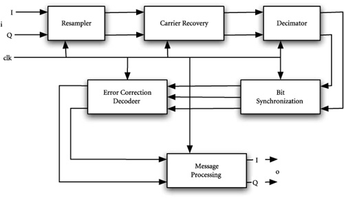
The definitions in Figure 19.2 are for the individual components comprising the structural block diagram from Figure 19.1 defining interfaces and functional elements. These definitions are no different than the functional models written for the original model. What is happening is that the functional definition is being pushed deeper into the design representation. This will always result when making design decisions.

facet interface resampler
 (i:: input complex; o:: output complex; clk:: input bit)::discrete_time is
end facet interface resampler;

facet interface carrierRecovery
 (i:: input complex; o:: output complex; clk:: input bit)::discrete_time is
end facet interface carrierRecovery;

facet interface decimator
 (i:: input complex; o:: output complex,clk:: input bit)::discrete_time is
end facet interface decimator;

facet interface bitSynchronization
 (i:: input complex; o:: output complex ,clk:: input bit)::discrete_time is
facet interface bitSynchronization;

facet interface errorCorrection
 (i:: input complex; o:: output complex,clk:: input bit)::discrete_time is
end facet interface errorCorrection;

facet interface messageProcessor
 (i:: input complex; o:: output complex ,clk:: input bit)::discrete_time is
end facet interface messageProcessor;

The structural design in Figure 19.3 accomplishes three modeling tasks. First, each component model is composed with the CMOS power consumption model and instantiated within the component. The result is a collection of specification products representing each component’s function and power consumption model. Next, interconnections are made between individual components and from components to the TDMA receiver interface. Finally, the power associated with the TDMA receiver is calculated by summing the powers from the individual components.

facet TDMAstruct
 (i::input complex; o::output complex; clk::input bit)::discrete_time is
  export power;
  power :: real;
  ec2mp,bs2ec,d2bs,cr2d,r2cr :: complex;
  gammaSBDT(f:state_based)::discrete_time is
    (state_based_infinite_state.gamma . infinite_state_discrete_time.gamma);

begin
  c1: resampler(i,r2cr,clk)
      * gammaSBDT(CMOSpowerConsumption(i,r2cr));
  c2: carrierRecovery(r2cr,cr2d,clk)
      * gammaSBDT(CMOSpowerConsumption(r2cr,cr2d));
  c3: decimator(cr2d,d2bs,clk)
      * gammaSBDT(CMOSpowerConsumption(cr2d,d2bs));
  c4: bitSynchronization(d2bs,bs2ec,clk)
      * gammaSBDT(CMOSpowerConsumption(d2bs,bs2ec));
  c5: errorCorrection(bs2ec,ec2mp,clk)
      * gammaSBDT(CMOSpowerConsumption(bs2ec,ec2mp));
  c6: messageProcessor(ec2mp,o,clk)
      * gammaSBDT(CMOSpowerConsumption(ec2mp,o));
  power' = power + c1.power + c2.power + c3.power
         + c4.power + c5.power + c6.power;
end facet TDMAstruct;

The result of this construction is somewhat different than earlier models in that it does not include the power constraint. The power value exportedfromthe model is the consumed power, not a power limit. There are two ways to include the power constraint. One is to simply compose the TDMA model with the power constraint at the component level. This is achieved using the state_based power constraint model and constructing the product with the structural TDMA after moving the state_based model to discrete_time:

TDMA(i:: input complex; o:: output complex; clk:: input bit)::discrete_time is
  TDMAstruct(i,o,clk) *
  state_based_infinite_state.gamma(
    infinite_state_discrete_time.gamma(powerConstraint_sb(i,o)));

An alternative approach is to budget power across components and add the power constraint model to each instantiated component. The distinction is that when composing the structural model with the the system power constraint, analysis will only reveal a problem at the systems level. It will not indicate the component or components causing the problem. By budgeting the power constraint across components, analysis will reveal problems at the component level. Unfortunately, the model from Figure 19.4 is unwieldy and defeats the separation-of-concerns goals that Rosetta promotes. An alternative mechanism exists to form the product model using a products of structural facets.

facet TDMAstruct
  (i:: input complex; o:: output complex; clk:: input bit)::discrete_time is
   export power;
   power :: real;
   ec2mp,bs2ec,d2bs,cr2d,r2cr :: complex;
   gammaSBDT(f:state_based)::discrete_time is
    (state_based_infinite_state.gamma . infinite_state_discrete_time.gamma);
begin
  c1: resampler(i,r2cr,clk)
      * (gammaSBDT(CMOSpowerConsumption(i,r2cr)
         * static_state_based.gamma(powerConstraint(1e-6))));
  c2: carrierRecovery(r2cr,cr2d,clk)
      * (gammaSBDT(CMOSpowerConsumption(r2cr,cr2d)
         * static_state_based.gamma(powerConstraint(2e-6))));
  c3: decimator(cr2d,d2bs,clk)
      * (gammaSBDT(CMOSpowerConsumption(cr2d,d2bs)
         * static_state_based.gamma(powerConstraint(1e-6))));
  c4: bitSynchronization(d2bs,bs2ec,clk)
      * (gammaSBDT(CMOSpowerConsumption(d2bs,bs2ec)
         * static_state_based.gamma(powerConstraint(3e-6))));
  c5: errorCorrection(bs2ec,ec2mp,clk)
      * (gammaSBDT(CMOSpowerConsumption(bs2ec,ec2mp)
         * static_state_based.gamma(powerConstraint(1e-6))));
  c6: messageProcessor(ec2mp,o,clk)
      * (gammaSBDT(CMOSpowerConsumption(ec2mp,o)
         * static_state_based.gamma(powerConstraint(1e-6))));
end facet TDMAstruct;

Figures 19.5 through 19.7 structurally model function, power constraints, and power consumption for the TDMA receiver model. These models are separate in the same sense that the original TDMA models were separate. Using the product, they are easily composed in the same manner as the individual models:

facet TDMAfunction
  (i:: input complex; o:: output complex; clk:: input bit)::discrete_time is
   export power;
   power :: real;
   ec2mp,bs2ec,d2bs,cr2d,r2cr :: complex;
begin
  c1: resampler(i,r2cr,clk);
  c2: carrierRecovery(r2cr,cr2d,clk);
  c3: decimator(cr2d,d2bs,clk);
  c4: bitSynchronization(d2bs,bs2ec,clk);
  c5: errorCorrection(bs2ec,ec2mp,clk);
  c6: messageProcessor(ec2mp,o,clk);
end facet TDMAfunction;

facet TDMApowerBudget()::discrete_time is
   export power;
    power :: real;
begin
 c1: static_state_based.gamma(powerConstraint(1e-6)));
 c2: static_state_based.gamma(powerConstraint(2e-6)));
 c3: static_state_based.gamma(powerConstraint(1e-6)));
 c4: static_state_based.gamma(powerConstraint(3e-6)));
 c5: static_state_based.gamma(powerConstraint(1e-6)));
 c6: static_state_based.gamma(powerConstraint(1e-6)));
 power = c1.power + c2.power + c3.power
       + c4.power + c5.power + c6.power;
end facet TDMApowerBudget;

facet TDMAconsumption
  (i:: input complex; o:: output complex)::discrete_time is
    export power;
    power :: real;
    ec2mp,bs2ec,d2bs,cr2d,r2cr :: complex;
    gammaSBDT(f:state_based)::discrete_time is
      (state_based_infinite_state.gamma . infinite_state_discrete_time.gamma);
begin
  c1: gammaSBDT(CMOSpowerConsumption(i,r2cr));
  c2: gammaSBDT(CMOSpowerConsumption(r2cr,cr2d));
  c3: gammaSBDT(CMOSpowerConsumption(cr2d,d2bs));
  c4: gammaSBDT(CMOSpowerConsumption(d2bs,bs2ec));
  c5: gammaSBDT(CMOSpowerConsumption(bs2ec,ec2mp));
  c6: gammaSBDT(CMOSpowerConsumption(ec2mp,o));
  power' = power + c1.power + c2.power + c3.power
         + c4.power + c5.power + c6.power;
end facet TDMAconsumption;

TDMA(i:: input complex; o:: output complex; clk:: input bit)::discrete_time is
  TDMAfunction(i,o,clk)
     * gammaSBDT(TDMAconsumption(i,o,clk)
       * static_state_based.gamma(TDMApowerBudget()));

This model is semantically identical to the previous model. The product operation is applied to each of the terms comprising the original structural models. Term labels are used to determine how the operations are applied. The product operations are distributed across like-named terms. For example, the c1 term resulting from the product is defined as:

TDMAfunction.c1
* gammaSBDT(TDMAconsumption.c1
        * static_state_based.gamma(TDMApowerBudget.c1));

Other terms are handled similarly, resulting in exactly the model defined earlier.

The final model combines the use of separate technology models and structural modeling. Figures 19.8 and 19.9 show functional and power decomposition of the receiver, respectively. Note the use of different models for different implementation technologies. Formation of the product model is identical to that in the previous example and results in a yet more accurate model.

facet TDMAconsumption
  (i::input complex; o::output complex)::discrete_time is
     export power;
     power :: real;
     ec2mp,bs2ec,d2bs,cr2d,r2cr :: complex;
     gammaSBDT(f:state_based)::discrete_time is
       (state_based_infinite_state.gamma . infinite_state_discrete_time.gamma);
begin
  c1: gammaSBDT(FPGApowerConsumption(i,r2cr));
  c2: gammaSBDT(CMOSpowerConsumption(r2cr,cr2d));
  c3: gammaSBDT(SWpowerConsumption(cr2d,d2bs));
  c4: gammaSBDT(FPGApowerConsumption(d2bs,bs2ec));
  c5: gammaSBDT(SWpowerConsumption(bs2ec,ec2mp));
  c6: gammaSBDT(SWpowerConsumption(ec2mp,o));
  power' = power + c1.power + c2.power + c3.power
         + c4.power + c5.power + c6.power;
end facet TDMAconsumption;

facet TDMAfunction
  (i::input complex; o::output complex; clk::input bit)::discrete_time is
     export power;
     power :: real;
     ec2mp,bs2ec,d2bs,cr2d,r2cr :: complex;
begin
  c1: FPGAresampler(i,r2cr,clk);
  c2: CMOScarrierRecovery(r2cr,cr2d,clk);
  c3: SWdecimator(cr2d,d2bs,clk);
  c4: FPGAbitSynchronization(d2bs,bs2ec,clk);
  c5: SWerrorCorrection(bs2ec,ec2mp,clk);
  c6: SWmessageProcessor(ec2mp,o,clk);
end facet TDMAfunction;

Mixed technology models are particularly useful when performing hardware/ software co-design. Such models may be automatically produced by synthesis tools and analysis results may be used to select the best implementation approach. Synthesis combinators also take advantage of these models by applying technology-specific synthesis techniques to individual functional components.

The objective of this case study is to explore alternatives to the initial power-aware case study and discuss refinement of system-level models. In this chapter, heterogeneous design is truly explored for the first time by allowing for different functional models for components using different implementation technologies. Additionally, the option of implementing different system functions simultaneously using different implementation technologies can be explored.

The introduction of technology-specific functional models has the greatest potential for increased modeling detail. As noted in Chapter 18, software uses a different underlying computational model and changes states in very different ways, as compared to hardware implementations of the same function. Technology-specific function models make it possible to define and analyze such systems. Using configurable models to select from among alternative technologies makes it simpler to configure and analyze models.

Structural decomposition is an important refinement step in any system design process. As design detail is added to functional models, it also propagates to constraint models. In effect, the constraint models follow design decisions, allowing more detailed and precise analysis. This evolution is vital as requirements flow through the design process or performance requirements become stale artifacts of initial design decisions.

When system components can be implemented using different technologies, we begin to explore the benefits of heterogeneity. Allowing models for components to be configurable over several implementation fabrics dramatically improves understanding of trade-offs among performance requirements and implementation fabrics. Using simulation, the system impacts of design fabrics and their interactions can be explored. If significant resources are brought to bear, one can imagine finding optimum or near-optimum implementations.